Tools and Resources

A community-maintained standard library of population genetic models

Department of Biology and Institute of Ecology and Evolution, University of Oregon, United States
Weatherall Institute of Molecular Medicine, University of Oxford, United Kingdom
Simons Center for Quantitative Biology, Cold Spring Harbor Laboratory, United States
Department of Genetics, University of North Carolina at Chapel Hill, United States
Lundbeck GeoGenetics Centre, Globe Institute, University of Copenhagen, Denmark
Department of Ecology and Evolutionary Biology, University of California, Los Angeles, United States
Department of Human Genetics, McGill University, Canada
Melbourne Integrative Genomics, School of Mathematics and Statistics, University of Melbourne, Australia
Department of Mathematical Stochastics, University of Freiburg, Germany
Department of Genome Sciences, University of Washington, United States
The Biodesign Institute and The School of Life Sciences, Arizona State University, United States
Department of Human Genetics, David Geffen School of Medicine, University of California, Los Angeles, United States
The Efi Arazi School of Computer Science, Herzliya Interdisciplinary Center, Israel
Department of Biology, Stanford University, United States
Department of Ecology, Evolution, and Environmental Biology, Columbia University, United States
Department of Computational BiologyCornell University, United States
Computer Technologies Laboratory, ITMO University, Russian Federation
International Laboratory for Human Genome Research, National Autonomous University of Mexico, Mexico
Departmentof Molecular and Cellular Biology, University of Arizona, United States
Department of Mathematics, University of Oregon, United States
Big Data Institute, Li Ka Shing Centre for Health Information and Discovery, University of Oxford, United Kingdom

Jun 23, 2020

https://doi.org/10.7554/eLife.54967

Open access
Copyright information

Figures
Tables
Additional files

15 figures, 1 table and 1 additional file

Figures

Figure 1

Download asset Open asset

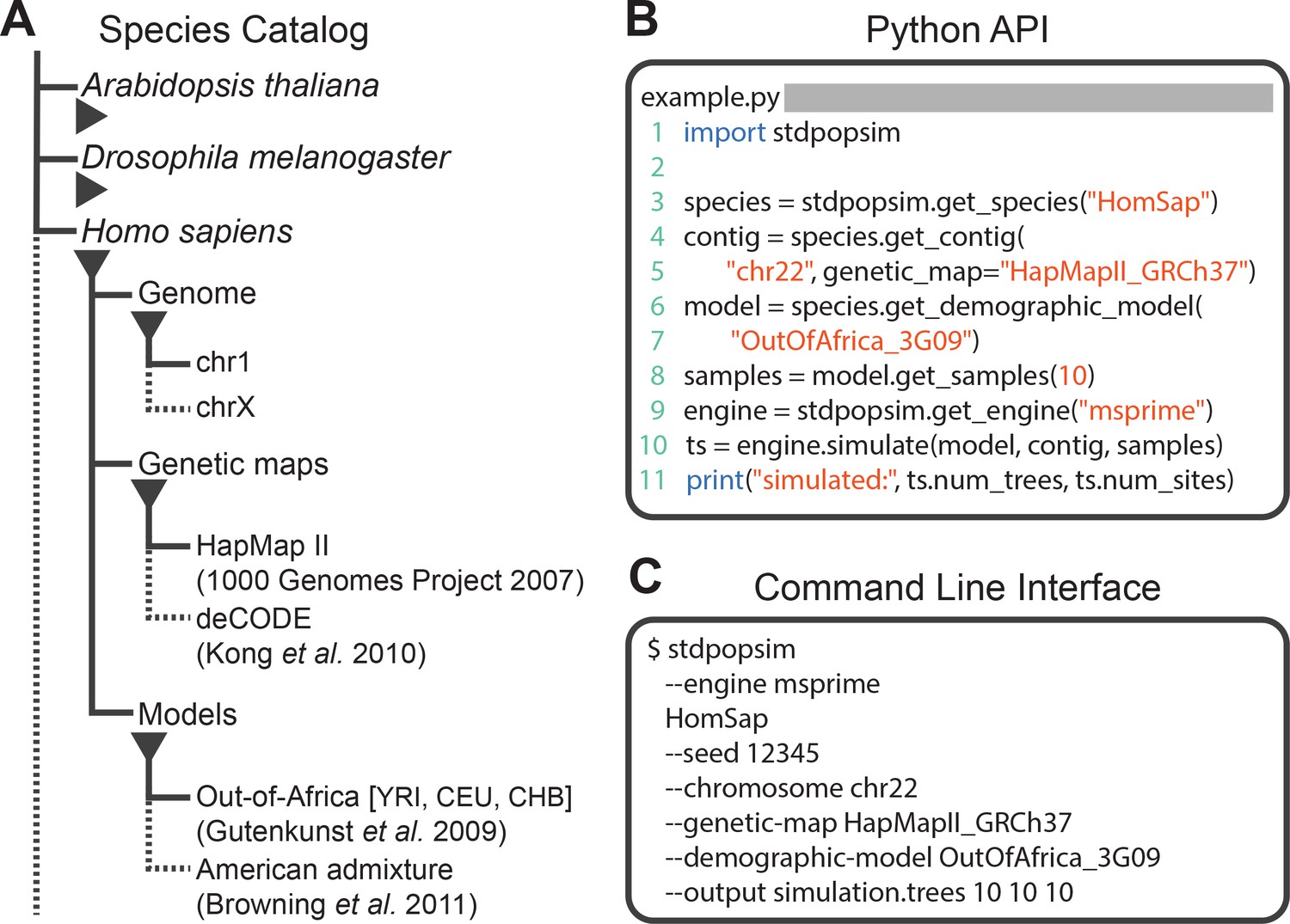
Structure of stdpopsim.

(A) The hierarchical organization of the stdpopsim catalog contains all model simulation information within individual species (expanded information shown here for *H. sapiens* only). Each species is associated with a representation of the physical genome, and one or more genetic maps and demographic models. Dotted lines indicate that only a subset of these categories is shown. At right we show example code to specify and simulate models using (B) the python API or (C) the command line interface.

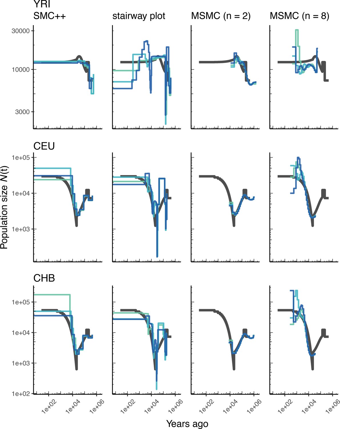
Figure 2

Download asset Open asset

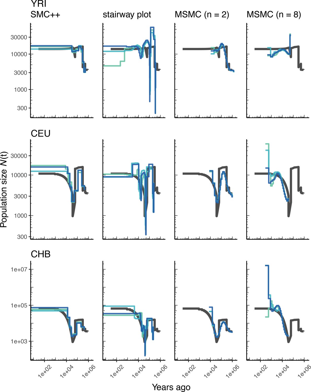
Comparing estimates of $N (t)$ in humans.

Here we show estimates of population size over time ( $N (t)$ ) inferred using four different methods: smc++, stairway plot, and MSMC with $n = 2$ and $n = 8$ samples. Data were generated by simulating replicate human genomes under the OutOfAfricaArchaicAdmixture_5R19 model (Ragsdale and Gravel, 2019) and using the HapMapII_GRCh37 genetic map (Frazer et al., 2007). From top to bottom, we show estimates for each of the three populations in the model (YRI, CEU, and CHB). In shades of blue we show the estimated $N (t)$ trajectories for each of three replicates. As a proxy for the ‘truth’, in black we show inverse coalescence rates as calculated from the demographic model used for simulation (see text).

Figure 3

Download asset Open asset

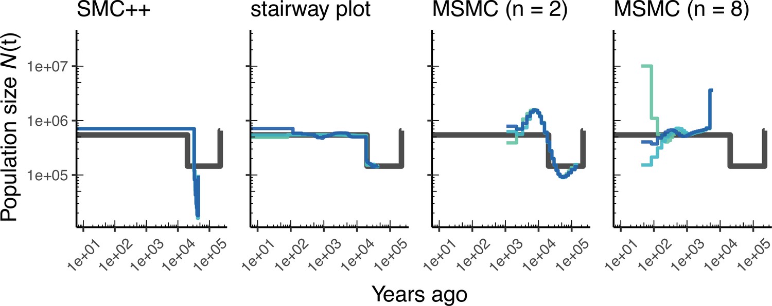
Comparing estimates of $N (t)$ in *Drosophila*.

Population size over time ( $N (t)$ ) estimated from an African population sample. Data were generated by simulating replicate *D. melanogaster* genomes under the African3Epoch_1S16 model (Sheehan and Song, 2016) with the genetic map of Comeron et al., 2012. In shades of blue we show the estimated $N (t)$ trajectories for each replicate. As a proxy for the ‘truth’, in black we show inverse coalescence rates as calculated from the demographic model used for simulation (see text).

Figure 4

Download asset Open asset

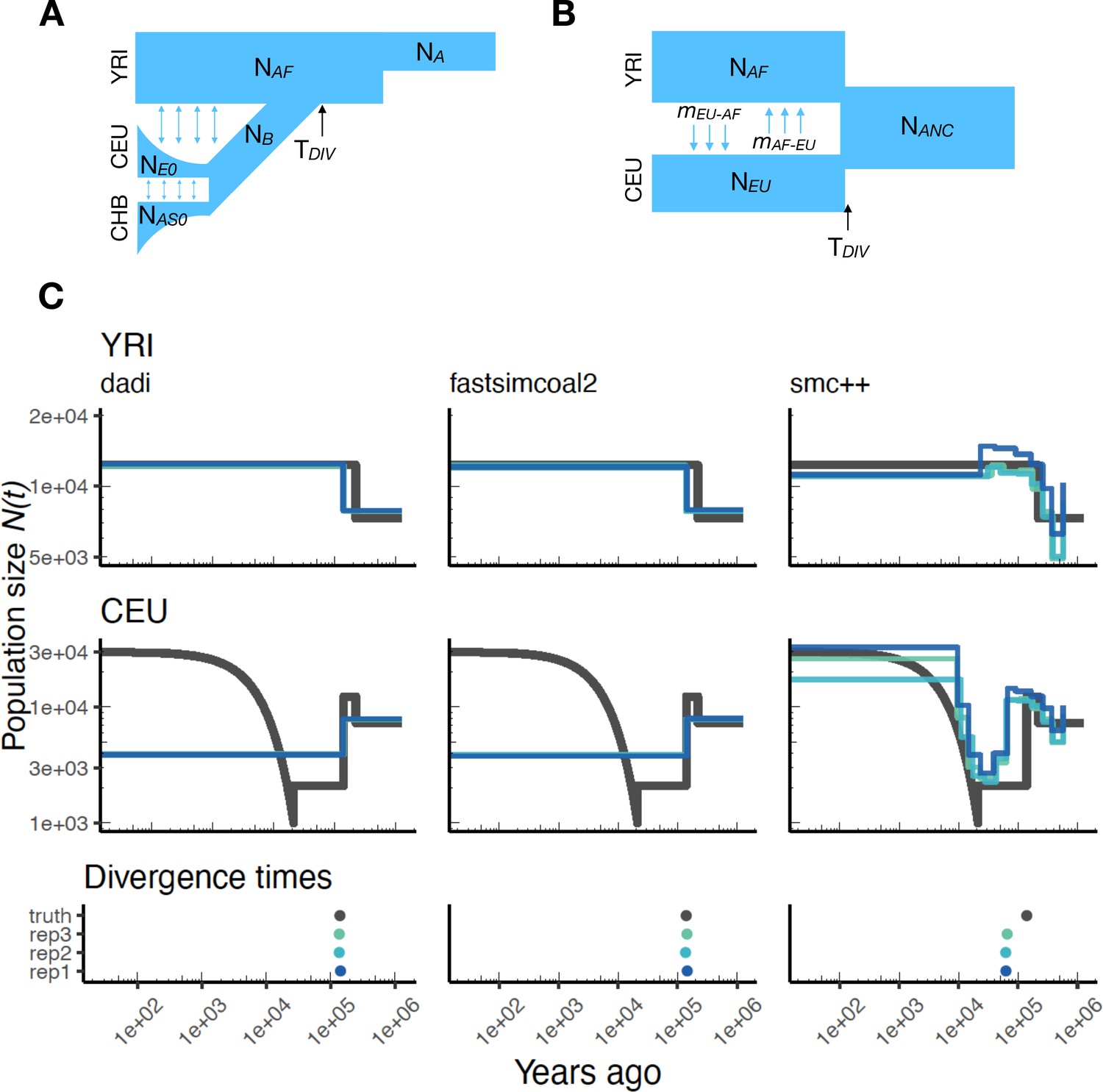
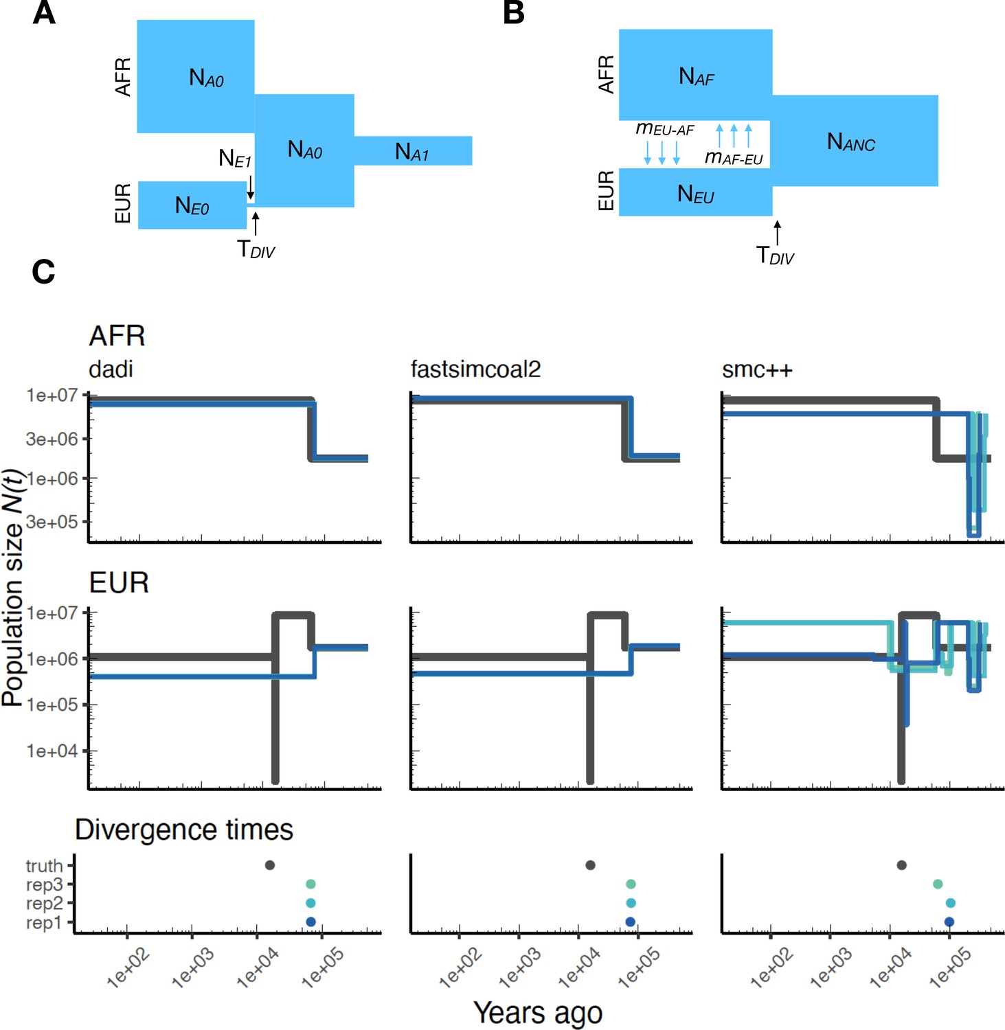
Parameters estimated using a multi-population human model.

Here we show estimates of $N (t)$ inferred using $\partial a \partial i$ , fastsimcoal2, and smc++. (A) Data were generated by simulating replicate human genomes under the OutOfAfrica_3G09 model and using the HapMapII_GRCh37 genetic map inferred in Frazer et al., 2007. (B) For $\partial a \partial i$ and fastsimcoal2 we show parameters inferred by fitting the depicted IM model, which includes population sizes, migration rates, and a split time between CEU and YRI samples. (C) Population size estimates for each population (rows) from $\partial a \partial i$ , fastsimcoal2, and smc++ (columns). In shades of blue we show $N (t)$ trajectories estimated from each simulation, and in black simulated population sizes for the respective population. The population split time, $T_{D I V}$ , is shown at the bottom (simulated value in black and inferred values in blue), with a common $x$ -axis to the population size panels.

Appendix 1—figure 1

Download asset Open asset

Validating the SLiM engine backend under a genetic map.

Here, we validate our integration of the SLiM (Haller et al., 2019; Haller and Messer, 2019) engine backend. We show quantile-quantile plots between SLiM and msprime engines for three population genetic summary statistics: r², Tajima’s $π$ , and Tajima’s D. Additionally, we show runtimes for generating each simulation replicate. Data were generated by simulating 100 replicates of human chromosome 22 under the AncientEurasia_9K19 model (Kamm et al., 2019) using the HapMapII_GRCh37 genetic map (Frazer et al., 2007). 12 samples were drawn from each population (excluding basal Eurasians). From top to bottom, we show results using three scaling factors for the population sizes: Q = 1, Q = 10, and Q = 50. Kolmogorov-Smirnov two-sample test statistics (D) and p-values are shown, testing the null hypothesis that the quantiles were drawn from the same continuous distribution.

Appendix 1—figure 2

Download asset Open asset

Validating the SLiM engine backend under uniform recombination.

Here, we validate our integration of the SLiM (Haller et al., 2019; Haller and Messer, 2019) engine backend. We show quantile-quantile plots between SLiM and msprime engines for three population genetic summary statistics: r², Tajima’s $π$ , and Tajima’s D. Additionally, we show runtimes for generating each simulation replicate. Data were generated by simulating 100 replicates of human chromosome 22 under the AncientEurasia_9K19 model (Kamm et al., 2019) using a uniform rate of recombination across the chromosome. 12 samples were drawn from each population (excluding basal Eurasians). From top to bottom, we show results using three scaling factors for the population sizes: Q = 1, Q = 10, and Q = 50. Kolmogorov-Smirnov two-sample test statistics (D) and p-values are shown, testing the null hypothesis that the quantiles were drawn from the same continuous distribution.

Appendix 1—figure 3

Download asset Open asset

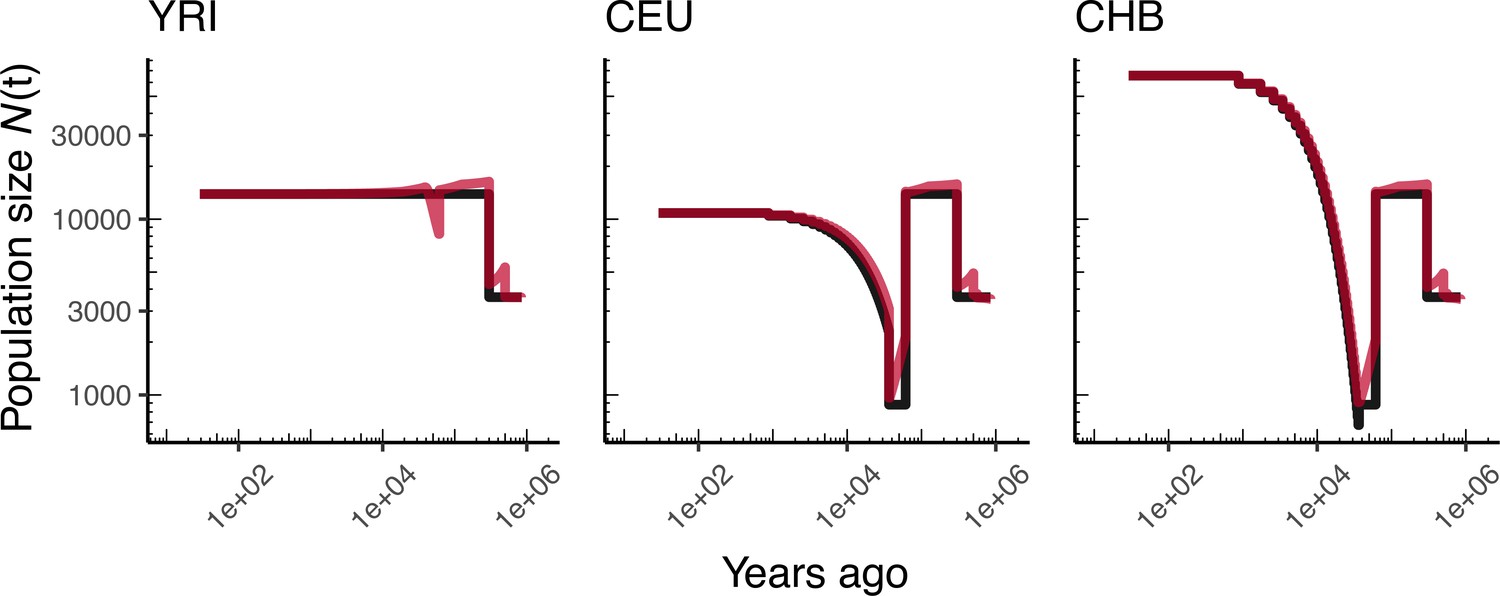
Comparing simulated population sizes and inverse coalescence rates in humans.

Data are shown from human genomes under the OutOfAfricaArchaicAdmixture_5R19 model (Ragsdale and Gravel, 2019) and using the HapMapII_GRCh37 genetic map (Frazer et al., 2007). From left to right, we show sizes for each of the three populations in the model: YRI, CEU, and CHB. We plot the simulated sizes for each population in black, and in red we plot inverse coalescence rates as calculated from the demographic model used for simulation (see text). In this specific model, these two measures are near identical, but in other models with higher migration rates we expect to see a larger departure between the two.

Appendix 1—figure 4

Download asset Open asset

Comparing estimates of $N (t)$ in humans.

Estimates of population size over time ( $N (t)$ ) inferred using four different methods, smc++, stairway plot, and MSMC with $n = 2$ and $n = 8$ . Data were generated by simulating replicate human genomes under the OutOfAfrica_3G09 model (Gutenkunst et al., 2009) and using the HapMapII_GRCh37 genetic map (Frazer et al., 2007). From top to bottom, we show estimates for each of the three populations in the model: YRI, CEU, and CHB. In shades of blue, we show the estimated $N (t)$ trajectories for each replicate. As a proxy for the ‘truth’, in black we show inverse coalescence rates as calculated from the demographic model used for simulation (see text).

Appendix 1—figure 5

Download asset Open asset

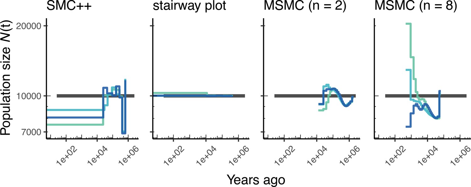
Comparing estimates of $N (t)$ in humans.

Here, we show estimates of population size over time ( $N (t)$ ) inferred using fourdifferent methods, smc+, and stairway plot, and MSMC with $n = 2$ and $n = 8$ . Data were generated by simulating replicate human genomes under a constant sized population model with $N = 10^{4}$ and using the HapMapII_GRCh37 genetic map (Frazer et al., 2007). As a proxy for the ‘truth’, in black we show inverse coalescence rates as calculated from the demographic model used for simulation (see text).

Appendix 1—figure 6

Download asset Open asset

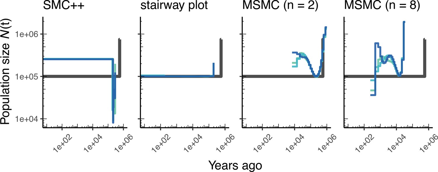
Comparing estimates of $N (t)$ in *A. thaliana*.

Here, we show estimates of population size over time ( $N (t)$ ) inferred using four different methods, smc++, and stairway plot, and MSMC with $n = 2$ and $n = 8$ . Data were generated by simulating replicate *A. thaliana* genomes under the African2Epoch_1H18 model (Durvasula et al., 2017) and using the SalomeAveraged_TAIR7 genetic map (Salomé et al., 2012). As a proxy for the ‘truth’, in black we show inverse coalescence rates as calculated from the demographic model used for simulation (see text).

Appendix 1—figure 7

Download asset Open asset

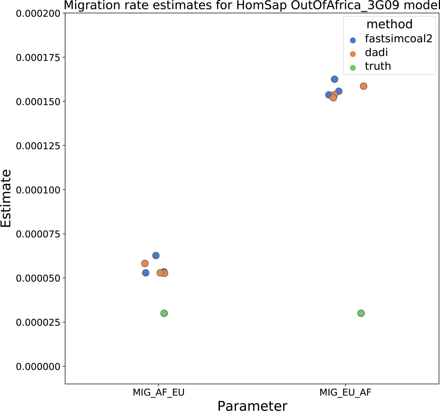
Migration rate estimates for the human Gutenkunst model.

Here, we show inferred migration rates from $\partial a \partial i$ and fastsimcoal2. Data were generated by simulating replicate human genomes under the Gutenkunst et al., 2009 model and using the genetic map inferred in Frazer et al., 2007. Directional migration from Europe to Africa is represented as $M I G_A F_E U$ and migration from Africa to Europe is represented as $M I G_E U_A F$ . Note that the $x$ -axis coordinates are arbitrary.

Appendix 1—figure 8

Download asset Open asset

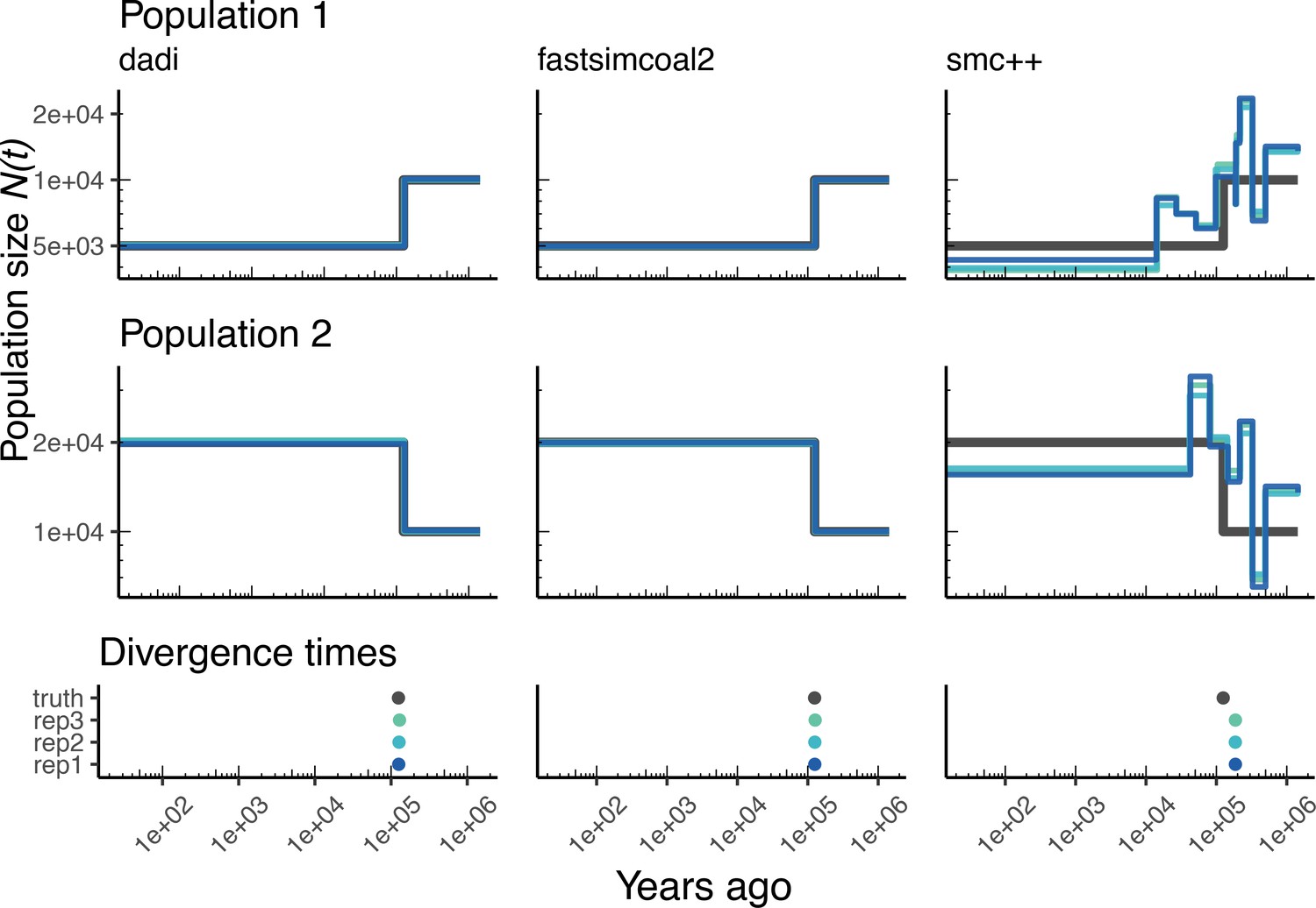
Parameters estimated using a two-population *Drosophila* model.

Here, we show estimates of $N (t)$ inferred using $\partial a \partial i$ , fastsimcoal2, and smc++. Data were generated by simulating replicate *Drosophila* genomes under the Li and Stephan, 2006 model and using the genetic map inferred in Comeron et al., 2012. See legend of Figure 4 for details. In shades of blue, we show the estimated $N (t)$ trajectories for each replicate. In black we show the simulated population sizes.

Appendix 1—figure 9

Download asset Open asset

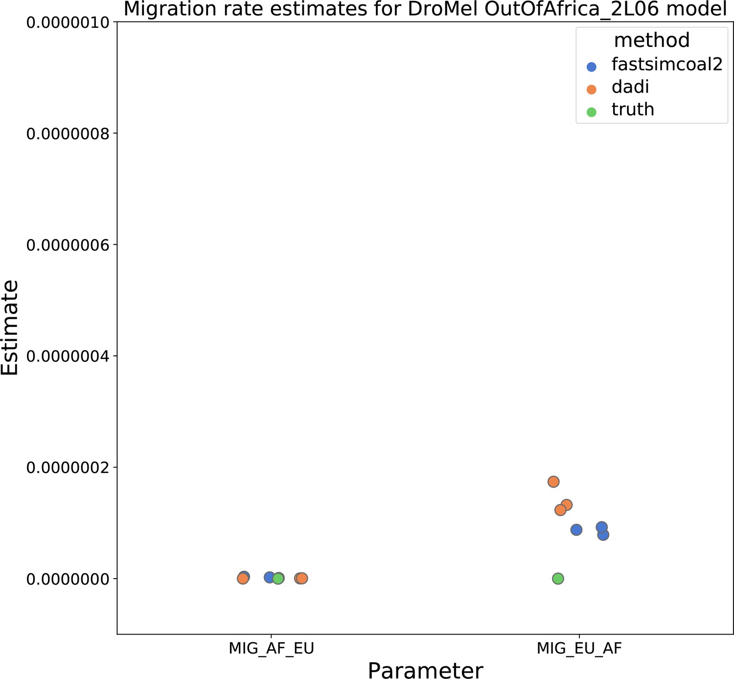
Migration rate parameters estimated under a two-population *Drosophila* model.

Here, we show inferred migration rates from $\partial a \partial i$ and fastsimcoal2. Data were generated by simulating replicate *Drosophila* genomes under the Li and Stephan, 2006 model and using the genetic map inferred in Comeron et al., 2012. Directional migration from Europe to Africa is represented as $M I G_A F_E U$ and migration from Africa to Europe is represented as $M I G_E U_A F$ . Note that the $x$ -axis coordinates are arbitrary.

Appendix 1—figure 10

Download asset Open asset

Workflow for our N(t) inference methods comparison.

Here, we show single replicate for two chromosomes, chr22 and chrX, simulated under the HomSap OutOfAfrica_3G09 demographic model, with a HapmapII_GRCh37 genetic map. Note that the data used as input by all inference methods smc++, MSMC, and stairway plot, come from the same set of simulations.

Appendix 1—figure 11

Download asset Open asset

Parameters estimated from a generic IM model Here we show estimates of $N (t)$ inferred using $\partial a \partial i$ , fastsimcoal2, and smc++.

Data were generated by simulating under a generic IM model with a human genome and Frazer et al., 2007 genetic map. In shades of blue we show the estimated $N (t)$ trajectories for each replicate. In black we show the simulated population sizes.

Tables

Table 1

Initial set of demographic models in the catalog and summary of computing resources needed for simulation.

For each model, we report the CPU time, maximum memory usage and the size of the output tskit file, as simulated using the msprime simulation engine (version 0.7.4). In each case, we simulate 100 samples drawn from the first population, for the shortest chromosome of that species and a constant chromosome-specific recombination rate. The times reported are for a single run on an Intel i5-7600K CPU. Computing resources required will vary widely depending on sample sizes, chromosome length, recombination rates and other factors.

Model ID	Citation	CPU(s)	Ram(MB)	File(MB)
HomSap (Homo sapiens)
Africa_1T12	Tennessen et al., 2012	10.0	194.2	23.3
Zigzag_1S14	Schiffels and Durbin, 2014	3.3	106.1	7.9
AshkSub_7G19	Gladstein and Hammer, 2019	13.8	216.3	26.4
OutOfAfrica_3G09	Gutenkunst et al., 2009	10.2	182.0	21.1
OutOfAfrica_2T12	Tennessen et al., 2012	10.7	198.4	24.1
AncientEurasia_9K19	Kamm et al., 2019	63.1	304.4	41.2
AmericanAdmixture_4B11	Browning et al., 2018	10.6	188.1	22.3
PapuansOutOfAfrica_10J19	Jacobs et al., 2019	204.5	524.7	77.8
OutOfAfricaArchaicAdmixture_5R19	Ragsdale and Gravel, 2019	8.8	185.4	21.7
DroMel (Drosophila melanogaster)
OutOfAfrica_2L06	Li and Stephan, 2006	252.8	678.0	106.7
African3Epoch_1S16	Sheehan and Song, 2016	3.0	123.9	11.5
AraTha (Arabidopsis thaliana)
African2Epoch_1H18	Huber et al., 2018	4.3	220.5	16.5
African3Epoch_1H18	Huber et al., 2018	2.6	241.3	18.4
PonAbe (Pongo abelii)
TwoSpecies_2L11	Locke et al., 2011	7.2	171.9	14.7