Random access parallel microscopy
- Department of Physiology, MGill University, Canada
- Department of Physics and Astronomy, University of Exeter, United Kingdom
- Department of Physics, Engineering Physics and Optics, Université Laval, Canada
Figures
Figure 1 with 2 supplements
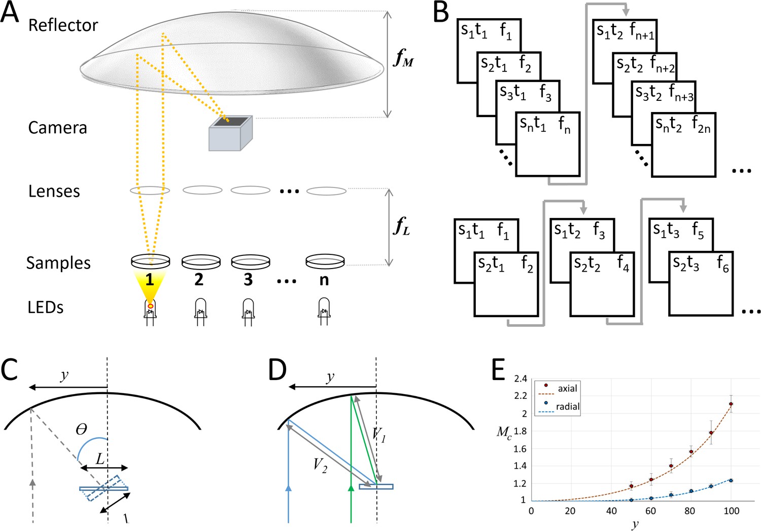
Random-access parallel (RAP) imaging principle and magnification properties.
(A) The random-access imaging system uses a parabolic reflector to image samples directly on a fast machine vision camera located at the focal point of the mirror (f M). Single-element plano-convex lenses are used as objectives, with samples positioned at their focal point (f L). Samples are sequentially illuminated using a LED array controlled by an Arduino microcontroller: a sample is only projected on the sensor when its corresponding LED is ‘on’. See Figure 1—figure supplement 1 and Table 1 for details. (B) (top) Sample s, is captured at time t, on frame f. For a total of n samples, each sample is captured once every n frames; (bottom) a smaller subset of samples can be imaged at higher temporal resolution by reducing the number of LEDs activated by the microcontroller. (C) Image magnification: the chief ray (dashed line) arrives at the detector plane at an incidence angle θ which increases with lateral displacement, y. The image is stretched in the direction parallel to y by a factor of L/l. (D) The image is isotopically magnified as the distance between the mirror and the image increases (V2>V1) as y increases. (E) The combined magnification, MC, shows the impact of the combined transformation on the magnification in both image dimensions (y' parallel to y, and x' orthogonal to y). Red dots (measured) and dashes (predicted) show magnification in y', and blue dots (measured) and dashes (predicted) show magnification in x', inset shows Images of a grid (200 μm pitch) taken with y = 70 mm, left is the uncorrected image and right shows the correct image using Equation 1.
Figure 1—figure supplement 1
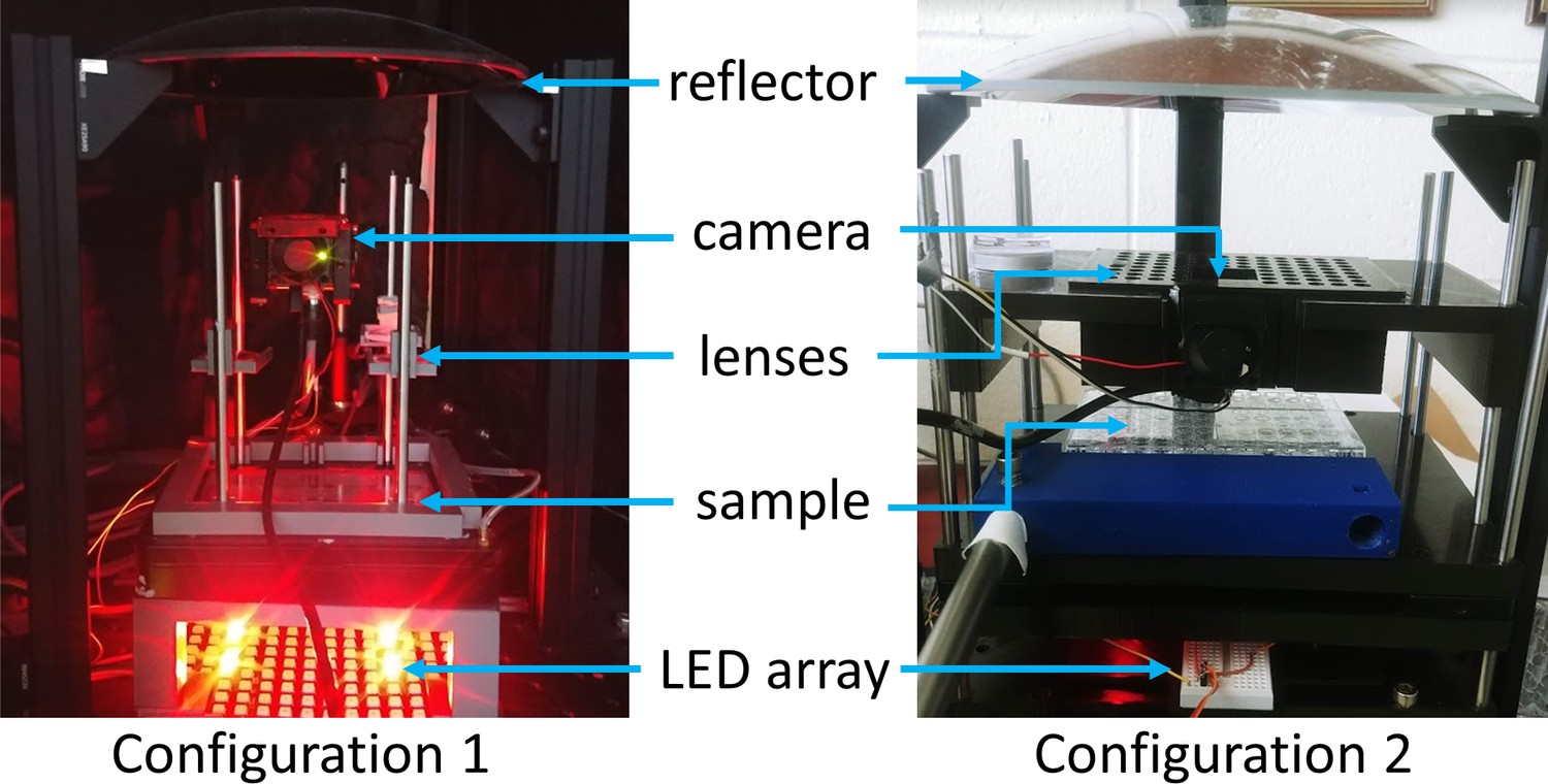
Configurations used for data collection.
Two configurations, constructed from a combination of Thorlabs optical components (Thorlabs ER series 6 mm rods) and 3D printed parts, were used to collect the data. Both configurations use the same parabolic reflector held at three points by optical rails (Thorlabs XE25) attached to a breadboard. Configuration 1 allows for adjustable focus for each sample by sliding a 3D printed lens holder along 6 mm diameter rods; Configuration 2 has an array of lenses at a fixed vertical position and focus is achieved by moving the samples (here a single 96-well plate).
Figure 1—figure supplement 2
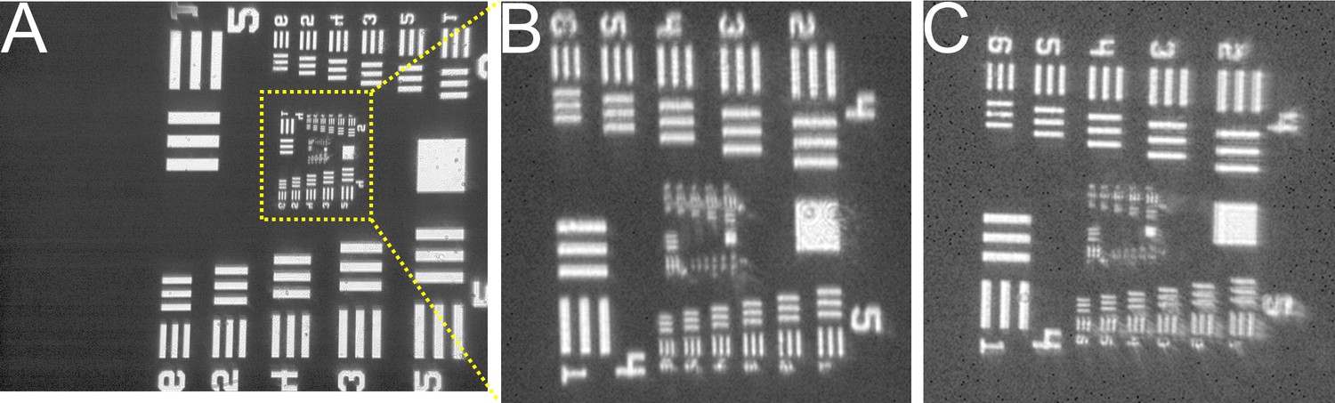
Comparison of conventional and RAP images.
USAF targets (clear pattern on a chrome background) imaged using 25 mm, 100 mm focal length plano-convex lens positioned 100 mm above the sample as an objective and the 100 mm focal length parabolic mirror to refocus the image (A, with a zoomed and flipped version of the same image shown in B) or a second 25 mm diameter, 100 mm focal length lens to refocus the image on the sensor (C, shown at same scale as B). The axial distance of the objective to the centre of the parabolic reflector is 40 mm (images A and B). The large square in the centre right in both close-up images is 140 × 140 μm. The sensor used is a 640 × 480 pixel camera with 4.8 × 4.8 μm pixels.
Figure 2
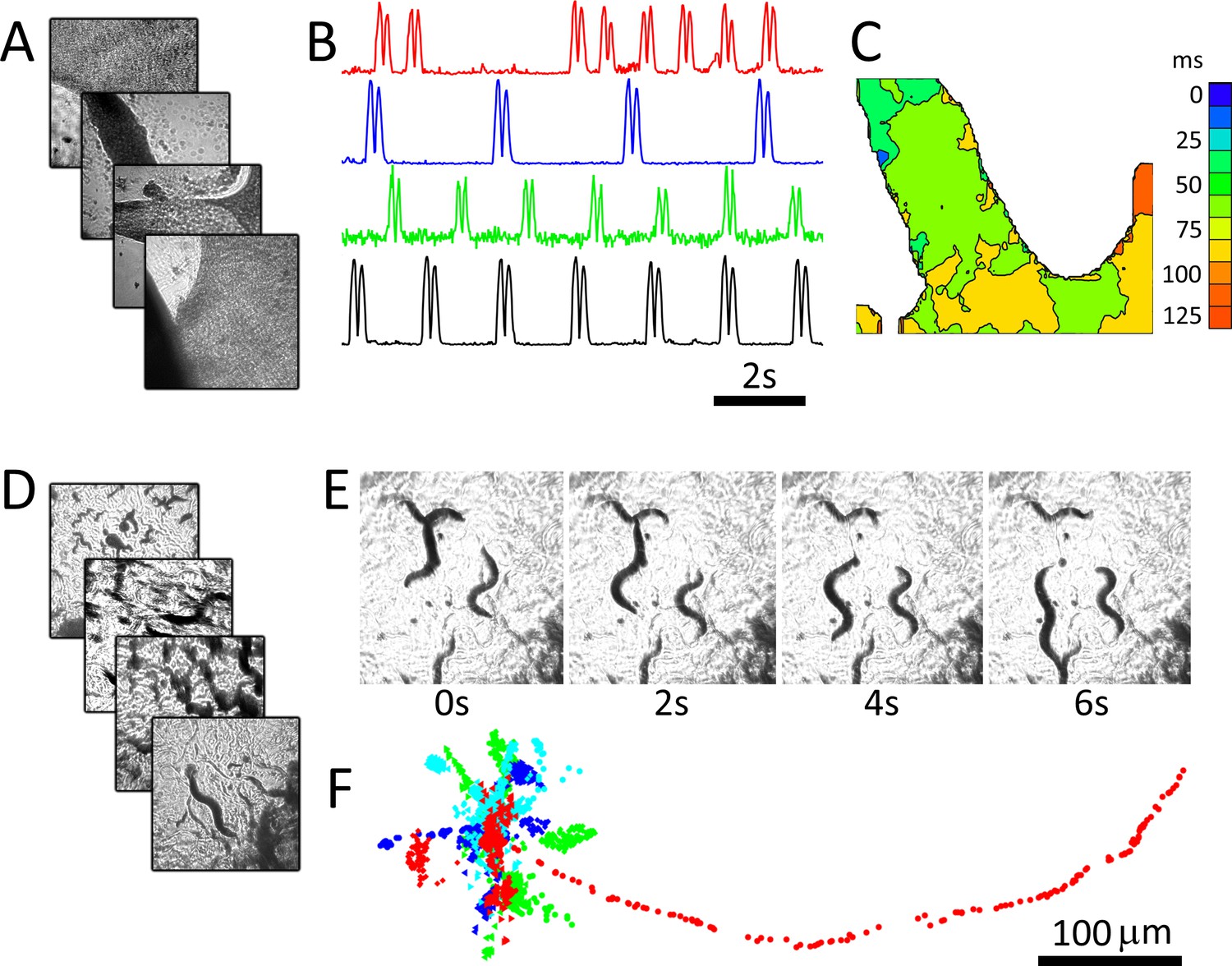
RAP imaging of cardiac monolayer and C. elegans preparations.
(A) Four cardiac monolayer preparations in four separate petri dishes are imaged in parallel at 40 fps/dish. (B) Activity vs time plots obtained from the four dishes show different temporal dynamics, where double peaks in each trace correspond to contraction and relaxation within a 20 × 20 pixel ROI (see Materials and methods); (C) an activation map from the second dish (blue trace in B) can be used to determine wave velocity and speed; (D) four C. elegans dishes imaged in parallel at 15 fps/dish; (E) images from one dish every 30 frames (2 s intervals) shows C. elegans motion; (F) the location of five worms in each dish was tracked from data recorded at 15 fps over 250 frames using open-source wrMTrck (Nussbaum-Krammer et al., 2015) software. Dots in different colours (blue, cyan, green, and red) show the tracked positions from plates 1–4, respectively. Each image in (A), (D), and (E) shows a 2 × 2 mm field of view.
Figure 3 with 1 supplement
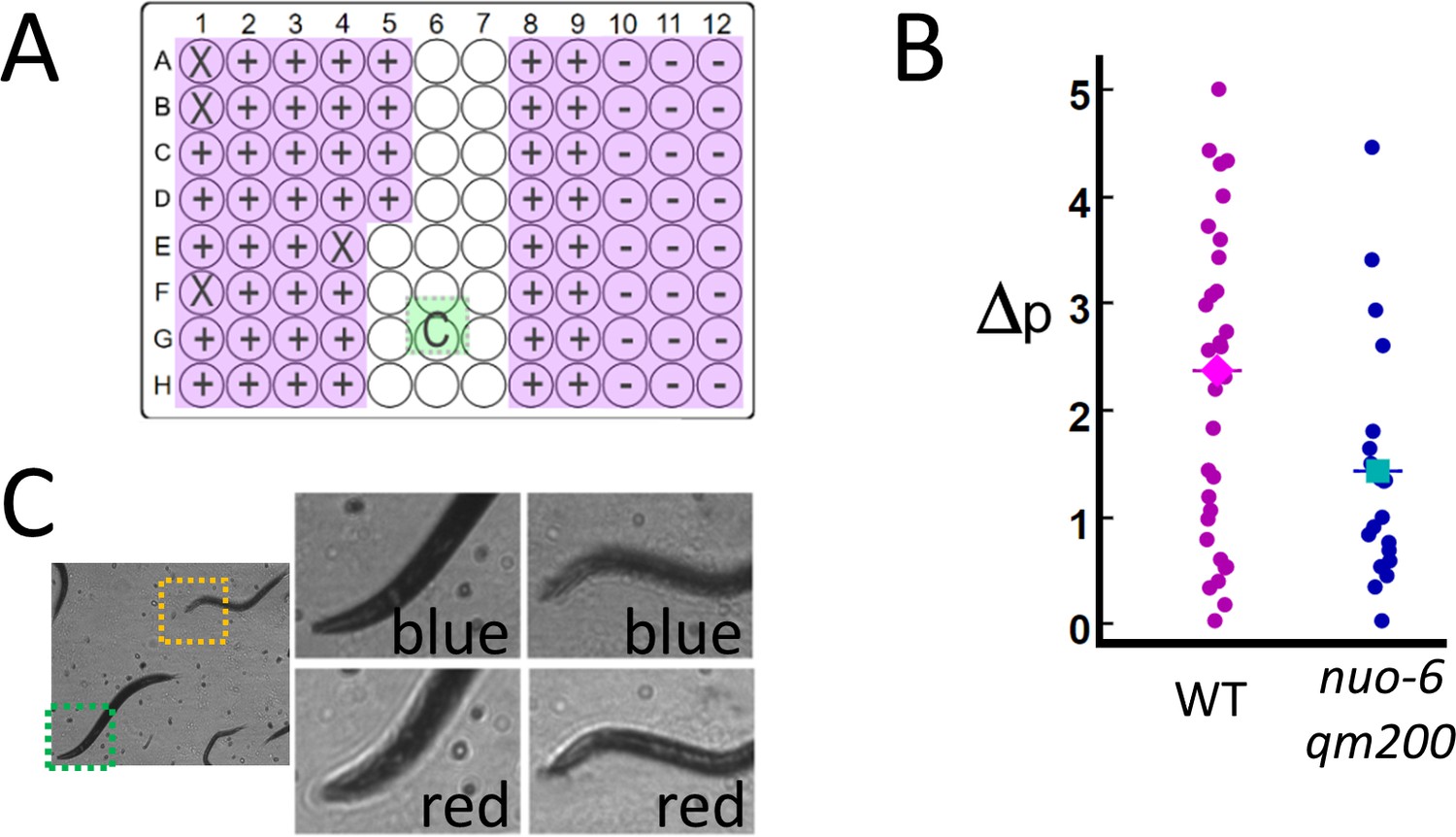
High-throughput estimates of C. elegans motion in liquid media.
Images are captured at 120 fps, which is split over multiple wells as shown in Video 1. (A) The position of the active detection sites (magenta) relative to the camera (green), which obscures a portion of the 96-well plate: Wells obscured by hardware are denoted by an ‘X’ symbol (see Materials and methods: Table 1), wells with wild-type C. elegans (WT, ‘+’ symbol) and mutant (nuo-6(qm200), ‘−’ symbol). (B) Motion analysis comparing wild type (magenta dots) to mitochondrial mutant nuo-6(qm200) (blue dots): wells in each row are imaged in parallel (eight wells at 15 fps per well), and net motion is estimated in each well by summing absolute differences in pixel intensities in sequential frames (see Materials and methods: Image analysis). This estimate confirms that the imaging system can detect significant differences between the two strains (averages shown by diamond and square symbols, two-tailed t-test p=0.01), which is consistent with published results (Yang and Hekimi, 2010). (C) Focal plane wavelength dependence: details from two fields of view (dashed green and orange squares) in the same image appear in or out of focus depending on whether imaged using a red or blue LED (see Video 2 and Figure 3—figure supplement 1).
Figure 3—figure supplement 1
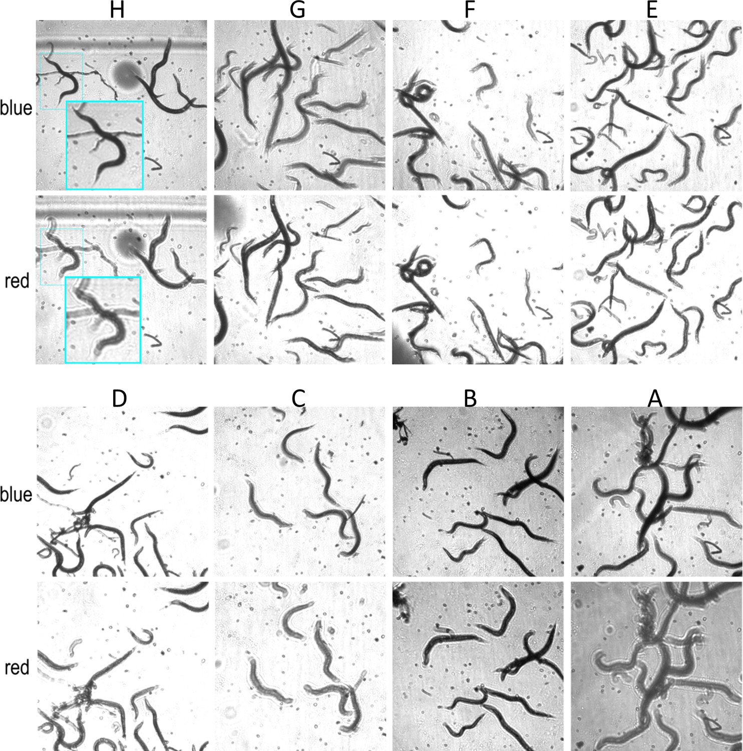
Focal plane wavelength dependence.
Images from all wells(A–H) for row 10, illuminated using a blue and red LEDs for Configuration 2 imaging C. elegans in liquid media. Images are in better focus when illuminated with the red LED for wells (G), (F), and (E) and the blue LED for wells (H), (D), (C), (B), and (A). Images for each channel are taken 8.3 ms apart, and the 16 images from eight wells are sampled at 7.5 fps. Each image is 512 × 512 pixels and is not transformed other than brightness adjustment in wells (B) and (A) for clarity. The inset in (H) shows a close up to highlight the focal plane difference between the two channels.
Author response image 1
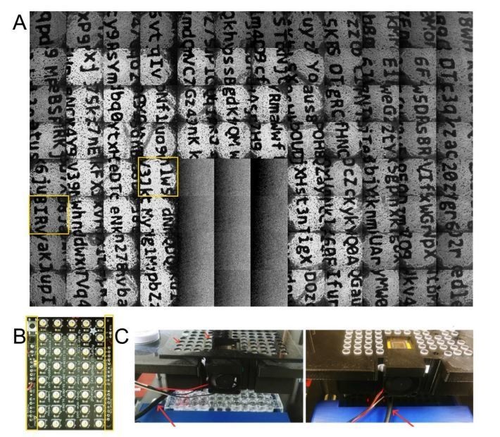
(A) composite image showing images from all wells aside from those under the camera housing, with wells obscured by cabling in Figure 3 highlighted in yellow.
(B) Image of one of the LED arrays with region reserved for electrical connections highlighted in yellow; the size of these regions prevents tiling the array and complete coverage of the 96 well plate (C) images of the system showing the location of the cable (red arrows) that obscured the wells in Figure 3, and its orientation for the image collected in the top panel of this figure (panel A).
Author response image 2
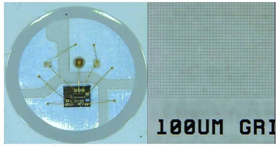
LED emitting area is approximately 200x200 microns.
Videos
Video 1
RAP recordings from a 96-well plate, showing recordings at different temporal resolutions.
Video 2
RAP recordings using different colours (red and blue LEDs) focus at different planes in the sample.
Tables
Table 1
Configuration details.
See Figure 1—figure supplement 1 for additional details.
| Configuration 1 | Configuration 2 | |
|---|---|---|
| Camera | Basler acA640-750um, 750 maximum fps, with 640 × 480, 4.8 × 4.8 μm pixels | Basler acA1300-200um, 202 maximum fps, with 1280 × 1024, 4.8 × 4.8 μm pixels |
| Lenses | Edmund Optics 25 mm diameter, 100 mm focal length (NA = 0.124) | Edmund Optics 6 mm diameter, 72 mm focal length (NA = 0.04) |
| LED array | Adafruit DotStar 8 × 32 LED matrix | 2× Adafruit NeoPixel 40 LED Shields |
| Sample location | Four samples equidistant (~40 mm) from the optical axis. | Up to 76 wells in a 96-well plate (Figure 3A). |
| Frame rate | Images captured at 160 fps for four sample (Figure 2A–C and 40.0 fps/sample) or 60 fps for four samples (Figure 2D–F and 15 fps/sample). | Images captured at 120 fps for eight samples (Figure 3 and 15 fps/sample). Different sampling rates are shown in Video 1. |
| Usage notes | Vibrations in cardiac experiments were damped by using Sorbothane isolators (Thorlabs AV5), and room light was blocked using black aluminium foil (Thorlabs BFK12). We use a 640 × 512 pixel ROI for the camera in Configuration 2 as the illumination spot is smaller than the camera FOV. Camera placement obscures 12 wells in the 96-well plate imaged in Configuration 2 (see Figure 3A), and the use of two commercial 40 element LED arrays precludes imaging all wells in a 96-well plate as the LEDs are permanently mounted on a board that is too large to be tiled without leaving gaps. In addition, some wells (marked in Figure 3A) were inadvertently obscured by hardware between the sample and objective lenses for the motion quantification experiment in Figure 3; however, the number of imaged wells was considered to be sufficient to demonstrate the utility of the RAP system. | |
Table 2
Comparison between conventional and RAP imaging systems.
| Conventional microscope | RAP microscope | |
|---|---|---|
| Resolution | NA = 0.025 (1×) to 0.95 (40×) | NA = 0.04 and 0.124 (1.4× and 1×) |
| Image quality | Optimal (multi-element objectives correct for most aberrations) | Moderate (single-element lenses used as objectives display spherical and other aberrations) |
| Modalities | Bright-field, phase contrast, DIC, fluorescence | Bright-field, multi-sample |
| Scan time* | ~8 min (no autofocus) ~11 min (with autofocus)† | 1 min (no focus) 2 min (LED colour switching) |
| Focal drift | Moderate to low (due to the use of a heavy machined platform, with further improvements afforded to autofocus systems) | Moderate to high (focal plane drift is expected due to light, 3D printed parts, but its impact can be mitigated by LED colour switching) |
| Cost | High (~$30,000 with automated x,y,z stages) | Low ($1750–$3250)‡ |
| Automation§ | Good (many automated microscopes are fully programmable) | Unknown (fully programmable, but not validated as part of a conventional high-throughput workflow) |
-
*Scan time is estimated for measuring the 72 unobstructed wells in a 96-well plate to allow direct comparison to the data in Figure 3. The estimate is based on moving serially between wells with a transit time of 0.5 s and imaging 100 frames at 15 fps. Examples from the literature vary considerably (e.g. up to one hour using 3D printed automation technologies, due to limitations in hardware communication speeds: see Schneidereit et al., 2017).
†We assume the autofocus algorithm takes on average 2.5 s (see Geusebroek et al., 2000).
-
‡The cost for the RAP system depends on the number of objective lenses used: Configuration 1 costs approximately $1750, while Configuration 2 (with 76 wells) costs approximately $3,250, as the cost for the cameras in both configurations are similar (~$400). Costs are in USD.
§‘Automation’ refers to a system’s ability to be integrated into robotic workflows. Conventional automated microscopes are core components of high-throughput screening platforms with sample and drug delivery capabilities. While our system is in principle compatible with these technologies (e.g. by leveraging existing open-source software, see Booth et al., 2018), it has not been tested in these settings.
Table 3
Comparison of image quality (intensity contrast and estimated lateral width of the point spread function) for varying distances from the optic axis.
| Off-axis distance (mm) | Contrast at 25 lp/mm | Estimated FWHM (μm) |
|---|---|---|
| 22.16 | 4.50 | 14.9 |
| 29.96 | 6.52 | 13.4 |
| 38.48 | 6.06 | 13.7 |
| 45.04 | 3.62 | 16.0 |
| 53.90 | 3.27 | 16.6 |
| 60.46 | 2.101 | 20.3 |
| 66.84 | 1.88 | 21.6 |
Additional files
-
Source code 1
Arduino code for controlling the camera and LED array for Configuration 1.
- https://cdn.elifesciences.org/articles/56426/elife-56426-code1-v3.zip
-
Source code 2
Python code for sorting images for each sample into unique directories.
- https://cdn.elifesciences.org/articles/56426/elife-56426-code2-v3.zip
-
Supplementary file 1
STL files and instructions for assembling RAP Configurations 1 and 2.
- https://cdn.elifesciences.org/articles/56426/elife-56426-supp1-v3.zip
-
Transparent reporting form
- https://cdn.elifesciences.org/articles/56426/elife-56426-transrepform-v3.pdf
Download links
A two-part list of links to download the article, or parts of the article, in various formats.
Downloads (link to download the article as PDF)
Open citations (links to open the citations from this article in various online reference manager services)
Cite this article (links to download the citations from this article in formats compatible with various reference manager tools)
Random access parallel microscopy
eLife 10:e56426.
https://doi.org/10.7554/eLife.56426


