Figures and data in Universality of clonal dynamics poses fundamental limits to identify stem cell self-renewal strategies

Figures
Tables
Additional files

20 figures, 2 tables and 1 additional file

Figures

Figure 1

Download asset Open asset

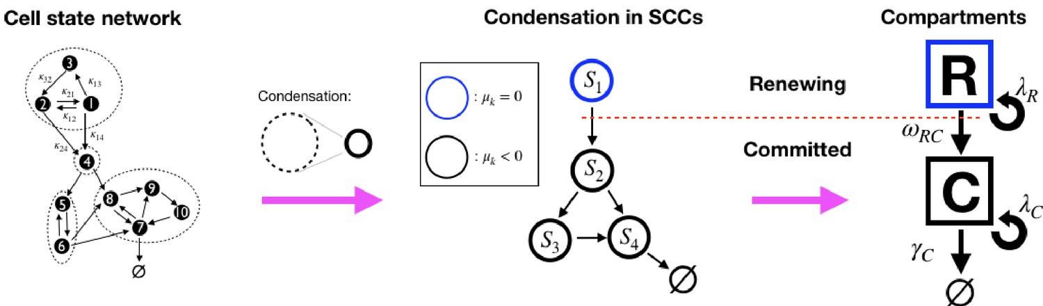
Illustration of the decomposition of a homeostatic cell state network into SCCs and the compartment representation, Equation 9.

(Left): An example cell state network representing the matrix $A$ in Equation 8 (self-links not displayed). The dashed circles denote the network’s Strongly Connected Components (SCCs ) (see definition in text). (Middle): The *Condensed network* is the corresponding network of SCCs, $S_{k}$ , wherein SCCs are the nodes and a link between two SCCs exists if any of their states are connected. For homeostatic networks, an SCC with dominant eigenvalue $μ = 0$ is at the apex, while other SCCs have $μ < 0$ . (Right): We distinguish two compartments, the Renewing compartment $ℛ$ , consisting of the apex SCC, with $μ = 0$ , and the Committed compartment $𝒞$ consisting of the remainder, with $μ < 0$ .

Figure 2

Download asset Open asset

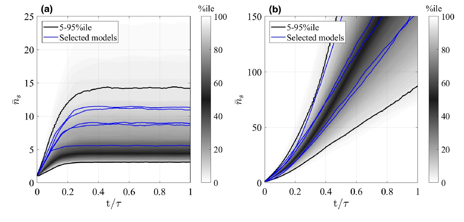
Mean size of surviving clones, ${\bar{n}}_{s}$ , as a function of time for random GIA models (a), and GPA models (b).

In (a), $τ = 20 / α_{\min}$ , in (b), $τ$ is the time at 98% clone extinction. The grey shade represents the percentile of all the simulations (black lines limit the 5-95%ile range); the blue curves correspond to some illustrative selected simulations. Simulations for which the final mean is below two and where the final condition is not achieved (due to computational limitations) are not included: this results in 238 and 571 models, respectively for the GIA and GPA cases.

Figure 3

Download asset Open asset

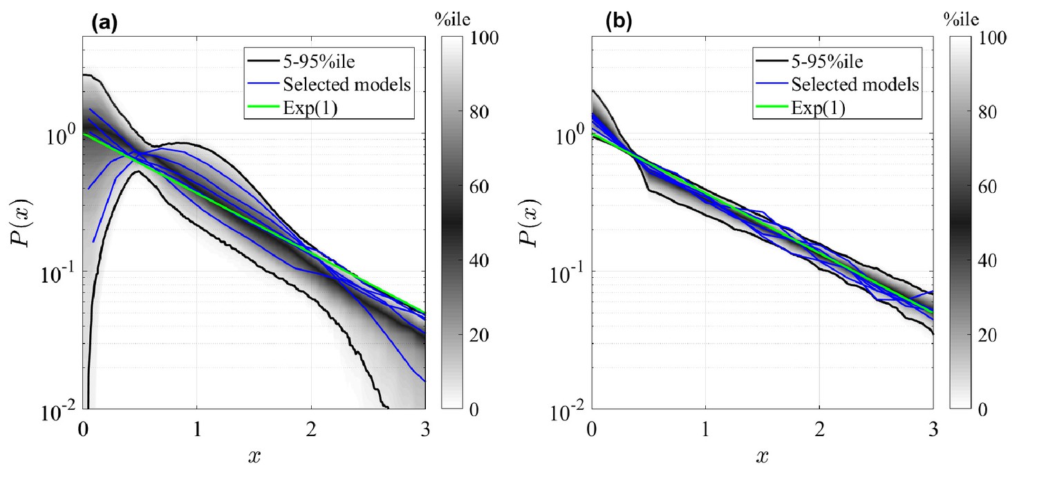
Rescaled clone size distributions (expected relative frequency $P$ of clone sizes) for random GIA models (a), and GPA models (b), in terms of the rescaled clone size $x = n / {\bar{n}}_{s}$ , at final time $t = τ$ (see Figure 2 for definition).

The grey shade represents the percentile of all the simulations (black lines limit the 5-95%ile range); the blue curves correspond to some selected simulations. A reference curve corresponding to an Exponential distribution of unitary mean (’Exp(1)’) is shown in green.

Figure 4

Download asset Open asset

Rescaled clone size distributions (expected relative frequency P of clone sizes) for random GIA models as in Figure 3, at time $t = τ$ (see definition in Figure 2).

Sensitivity to parameter ${\hat{λ}}_{R}$ is shown for one illustrative case in panel (a), and all GIA models for ${\hat{λ}}_{R} = 30$ in panel (b). The distributions are shown in terms of the rescaled variables $x = n / {\bar{n}}_{s}$ for panel (a) and $\tilde{x} = (n - {\bar{n}}_{s}) / σ_{n}$ , where $σ_{n}$ is the distributions variance, in panel (b). In (b), the grey shade represents the percentile of all simulations (black lines limit the 5-95%ile range); the blue curves correspond to some selected simulations. A reference curve corresponding to a Normal distribution of zero mean and unitary variance is shown in green. Simulations for which $t = τ$ is not reached (due to computational limitations) are not included, resulting in 922 model instances.

Appendix 1—figure 1

Download asset Open asset

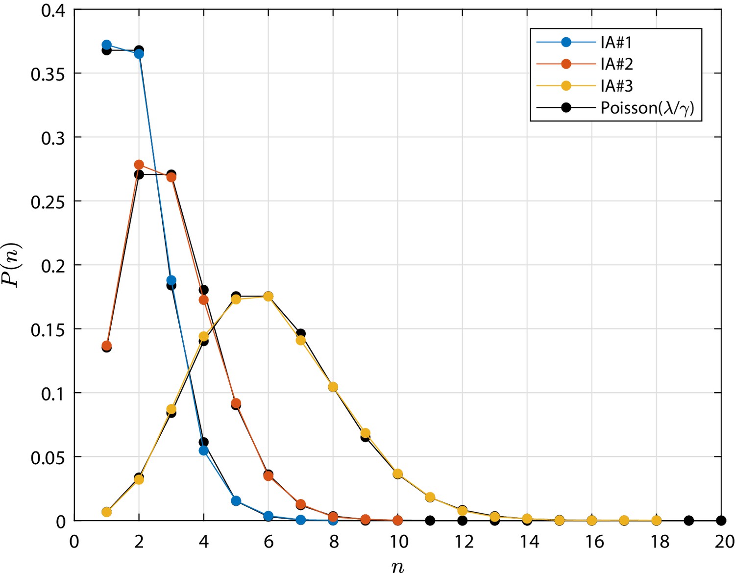
Invariant Asymmetry (IA) test cases clone size distribution $P (n)$ , that is the distribution of the total number of cells n forming the progeny of a single initial cell in $ℛ$ .

For each case, the distribution is shown at τ (defined in Figure 2, main text), which is well representative of the steady state condition. Tested parameters for cases IA#1-3 are provided in Appendix 1—table 1; the numerical simulation results are compared to the expected Poisson distribution. The detailed discussion is reported in 'Invariant Asymmetry and Population Asymmetry models'.

Appendix 1—figure 2

Download asset Open asset

Population Asymmetry (PA) test cases clone size distribution $P (n)$ , that is the distribution of the total number of cells n forming the progeny of a single initial stem cell.

For each case, the distribution is shown at the final time τ, at which the total extinction of the process is not yet achieved. Tested parameters for cases PA#-3 are provided in Appendix 1—table 1; the numerical simulation results are compared to the solution of the numerical integration of the master Equation 8 and, for test case PA#1, also to the reference analytic solution from Antal and Krapivsky, 2010. The detailed discussion is reported in 'Invariant Asymmetry and Population Asymmetry models'.

Appendix 1—figure 3

Download asset Open asset

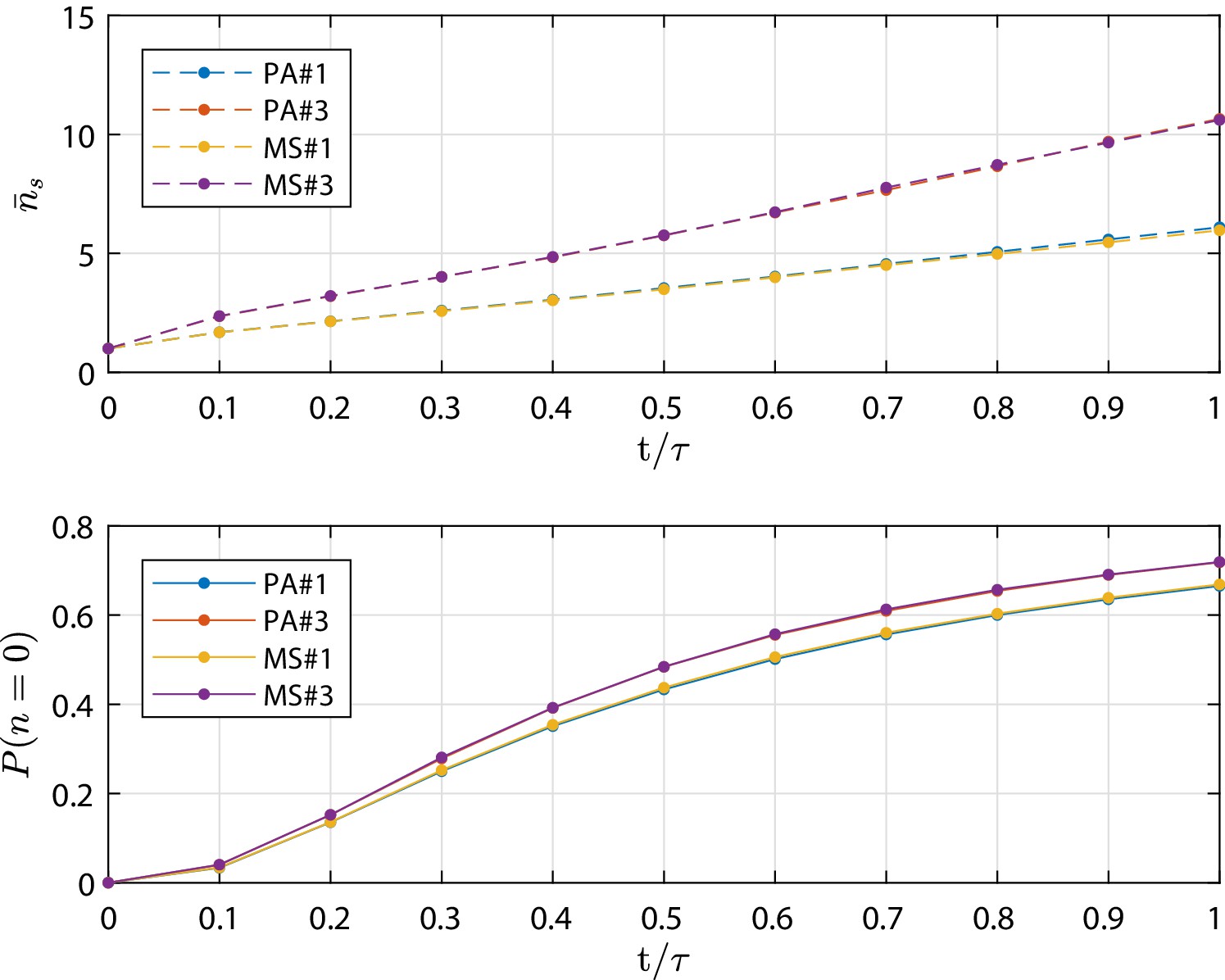
Metastate (MS) test cases simulation results in terms of mean number of cells in the surviving clones ${\bar{n}}_{s}$ and extinction probability $P (n = 0)$ as function of time (scaled by the final simulation time τ).

As well as for the PA test cases, at τ the total extinction of the process is not yet achieved. Profiles from the numerical simulation for cases MS#,3 are compared to the corresponding PA#1,3 test cases which are based on parameters provided in Appendix 1—table 1. The detailed discussion is reported in 'Population Asymmetry model using metastates'.

Appendix 1—figure 4

Download asset Open asset

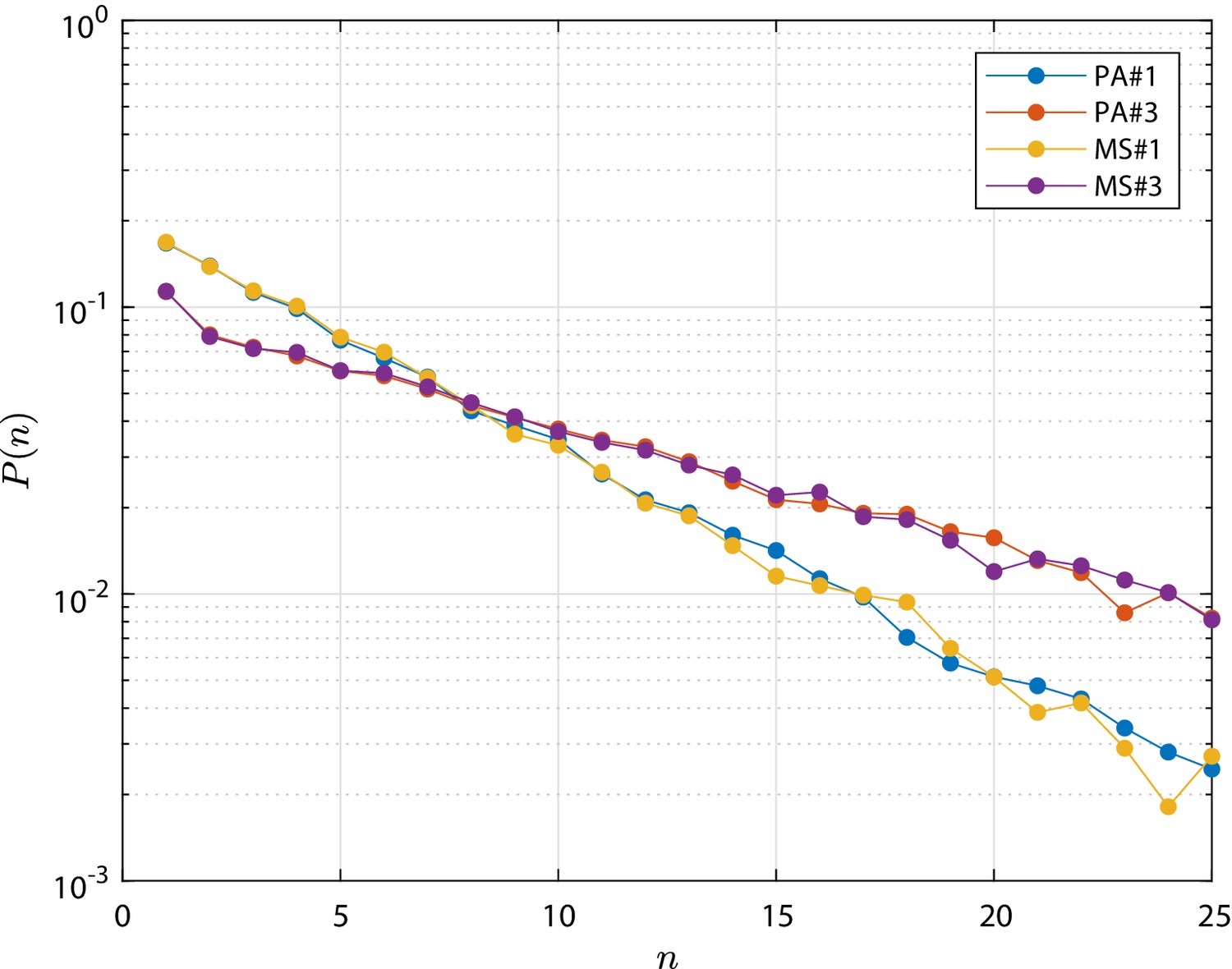
Metastate (MS) test cases simulation results in terms clone size distribution $P (n)$ , that is the distribution of the total number of cells n forming the progeny of a single initial stem cell.

As well as for the PA test cases, the distribution is shown at the final time, τ, at which the total extinction of the process is not yet achieved. Profiles from the numerical simulation for cases MS#,3 are compared to the corresponding PA#1,3 test cases which are based on parameters provided in Appendix 1—table 1. The detailed discussion is reported in 'Population Asymmetry model using metastates'.

Appendix 1—figure 5

Download asset Open asset

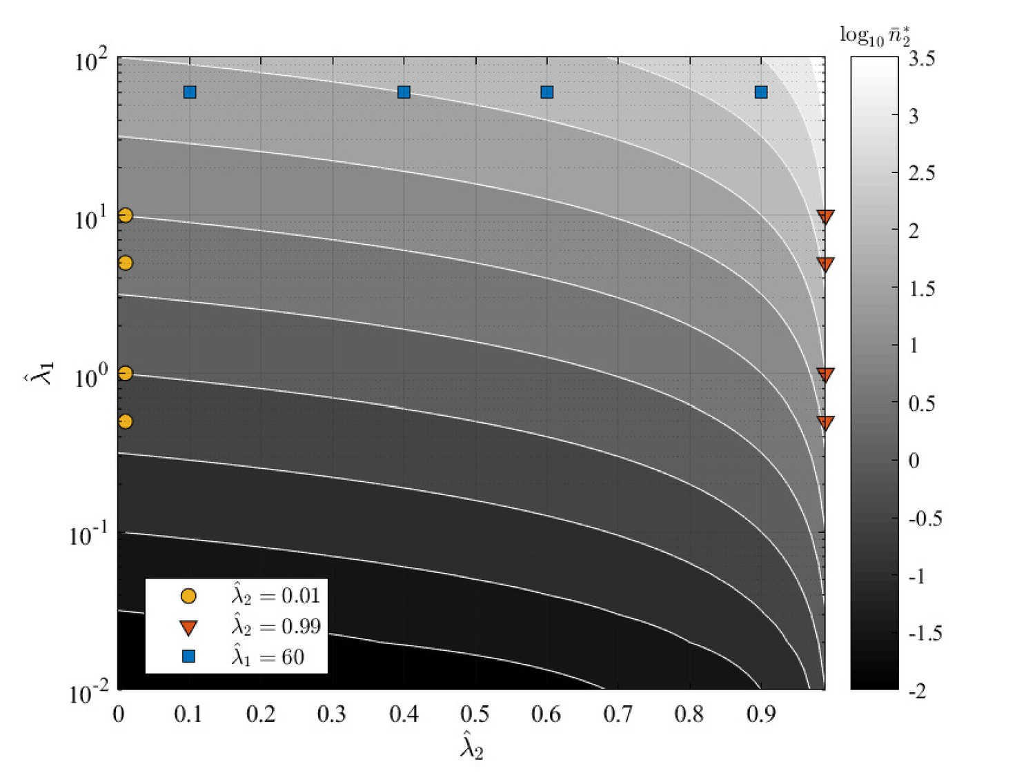
GIA⁰ test case parameters ${\hat{λ}}_{1}$ and ${\hat{λ}}_{2}$ over the contour map of the expected steady state mean number of cells in state $X_{2}$ , ${\bar{n}}_{2}^{*}$ .

The tested conditions are divided in three groups representing the limiting behaviors discussed in in 'GIA⁰ test case: steady state distribution and limiting behavior', and for which the steady state distribution is shown respectively in Appendix 1—figure 6, Appendix 1—figure 7 and Appendix 1—figure 8.

Appendix 1—figure 6

Download asset Open asset

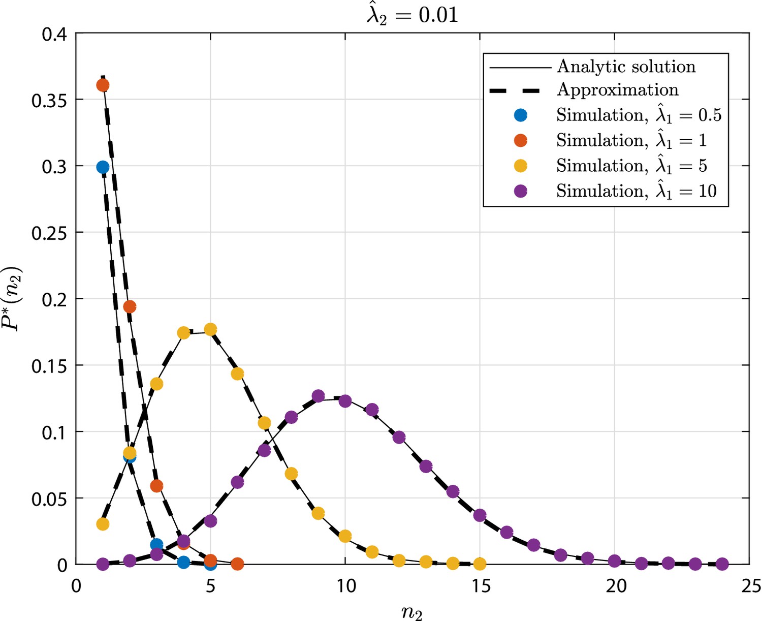
GIA⁰ test case (see GIA⁰ test case: steady state distribution and limiting behavior') results in terms of steady state distribution $P^{*} (n_{2})$ of the the number of cells in state $X_{2}$ , $n_{2}$ .

The tested parameters correspond to the condition ${\hat{λ}}_{2} = 0.01$ , as representative of the limiting case ${\hat{λ}}_{2} \to 0$ , and to different values of ${\hat{λ}}_{1}$ . The results from the numerical simulations are compared to the analytic solution (Equation 20), and its approximation, that is, the Poisson distribution (Equation 27).

Appendix 1—figure 7

Download asset Open asset

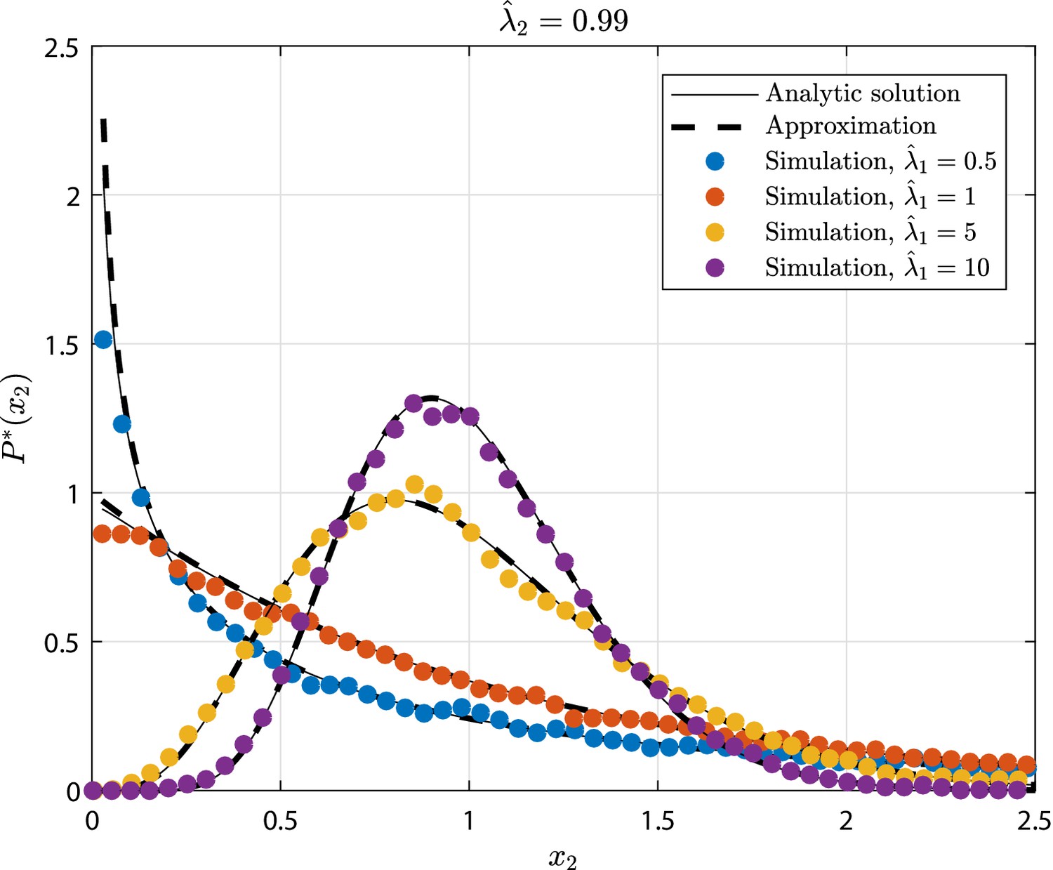
GIA⁰ test case (see 'GIA⁰ test case: steady state distribution and limiting behavior') results in terms of steady state rescaled distribution $P^{*} (x_{2})$ of the the number of cells in state $X_{2}$ , where $x_{2} = n_{2} / {\bar{n}}_{2}^{*}$ .

The tested parameters correspond to the condition ${\hat{λ}}_{2} = 0.99$ , as representative of the limiting case ${\hat{λ}}_{2} \to 1$ , and to different values of ${\hat{λ}}_{1}$ . The results from the numerical simulations are compared to the analytic solution (Equation 23), and its approximation that is the Gamma distribution (Equation 34).

Appendix 1—figure 8

Download asset Open asset

Appendix 1—figure 9

Download asset Open asset

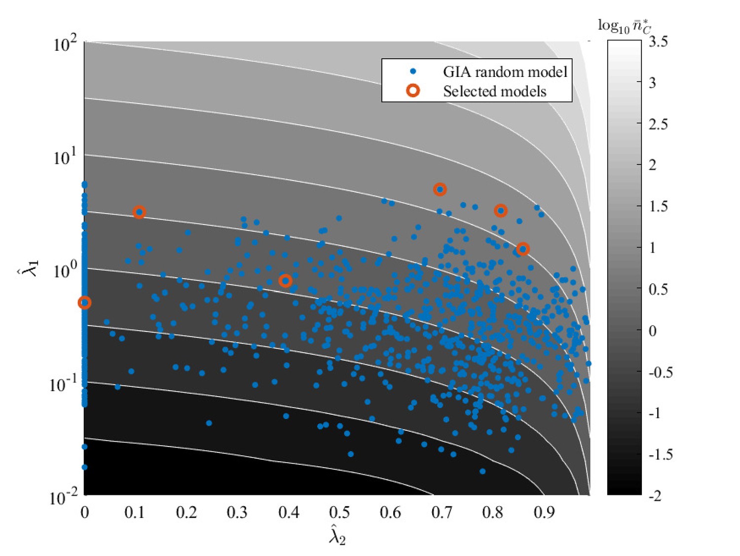
GIA random models (generated as described in 'Generation of random models' and analyzed in the main text) equivalent parameters ${\hat{λ}}_{1} = {\hat{λ}}_{R}$ and ${\hat{λ}}_{2} = {\hat{λ}}_{C}$ (see section Approximation of generic GIA models) over the contour map of the expected steady state mean number of cells in the committed compartment, ${\bar{n}}_{C}^{*}$ .

Some illustrative cases, for which the steady state distribution is shown in Appendix 1—figure 11, Appendix 1—figure 12 and Appendix 1—figure 13, are highlighted.

Appendix 1—figure 10

Download asset Open asset

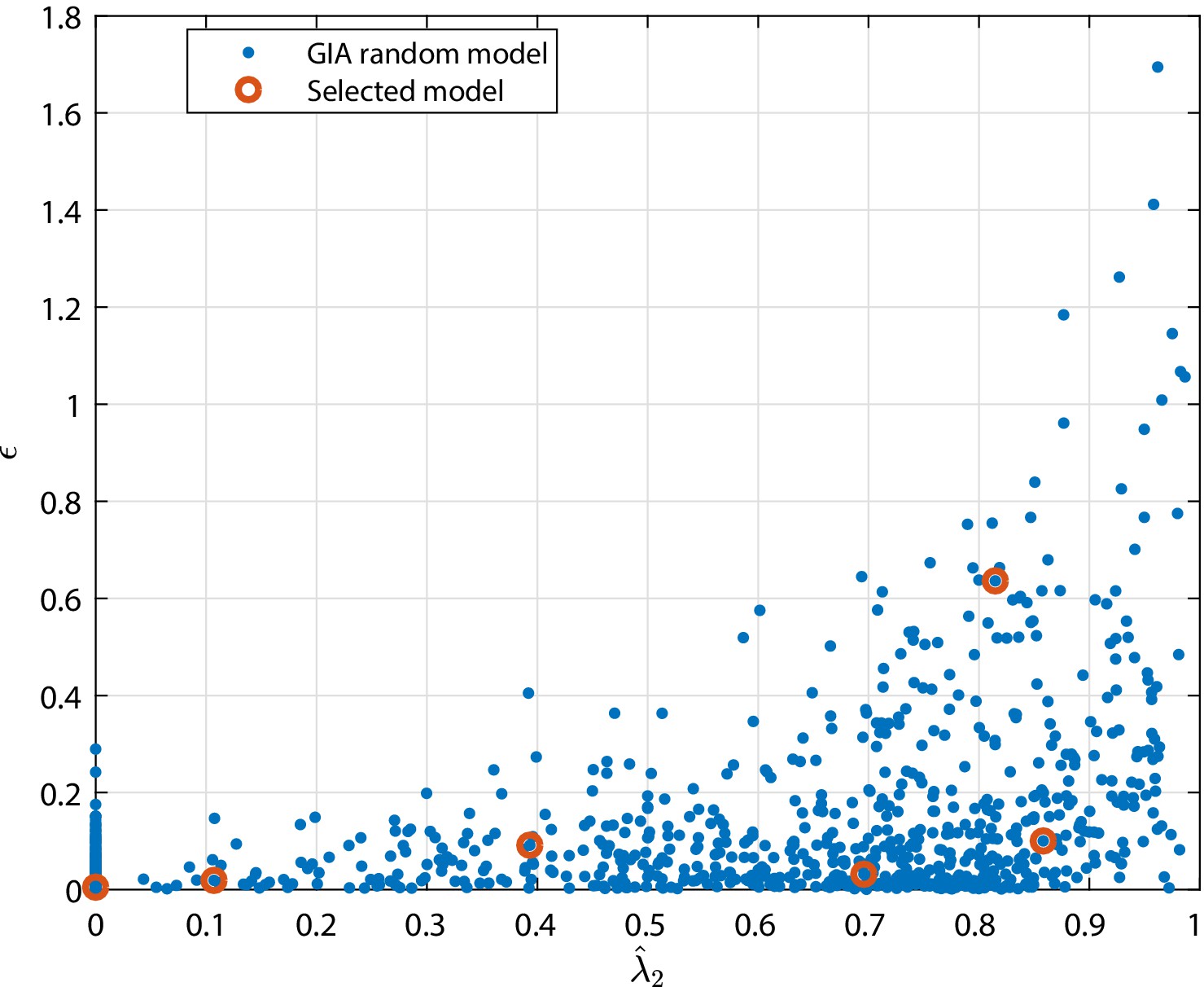
Relative error of the the equivalent model approximation, $ϵ$ , (see definition in 'Approximation of generic GIA models') as function of ${\hat{λ}}_{2} = {\hat{λ}}_{C}$ for the GIA random models (generated as described in 'Generation of random models' and analyzed in the main text).

The selected cases correspond to some illustrative cases for which the steady state distribution is shown in Appendix 1—figure 11, Appendix 1—figure 12 and Appendix 1—figure 13.

Appendix 1—figure 11

Download asset Open asset

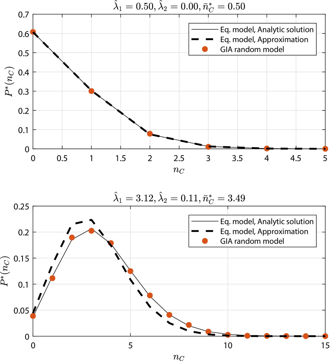
GIA random models selected cases (see Appendix 1—figure 9 and Appendix 1—figure 10) where ${\hat{λ}}_{2} < 0.2$ : the steady state distribution $P^{*} (n_{C})$ of the number of cells in the committed compartment, $n_{C}$ , is compared to that of the equivalent model (Equation model in the legend) analytic solution and its approximation for low ${\hat{λ}}_{2}$ (i.e. the Poisson distribution, Poisson $({\hat{λ}}_{1})$ ).

Results discussion is reported in 'Approximation of generic GIA models'.

Appendix 1—figure 12

Download asset Open asset

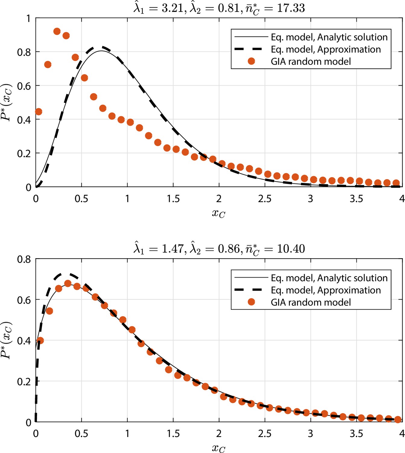
GIA random models selected cases (see Appendix 1—figure 9 and Appendix 1—figure 10) where ${\hat{λ}}_{2} > 0.8$ : the steady state rescaled distribution $P^{*} (x_{C})$ of the number of cells in the committed compartment, where $x_{C} = n_{C} / {\bar{n}}_{C}^{*}$ , is compared to that of the equivalent model (Equation model in the legend) analytic solution and its approximation for high ${\hat{λ}}_{2}$ (i.e. the Gamma distribution, Gamma $({\hat{λ}}_{1}, 1 / {\hat{λ}}_{1})$ ).

Results discussion is reported in 'Approximation of generic GIA models'.

Appendix 1—figure 13

Download asset Open asset

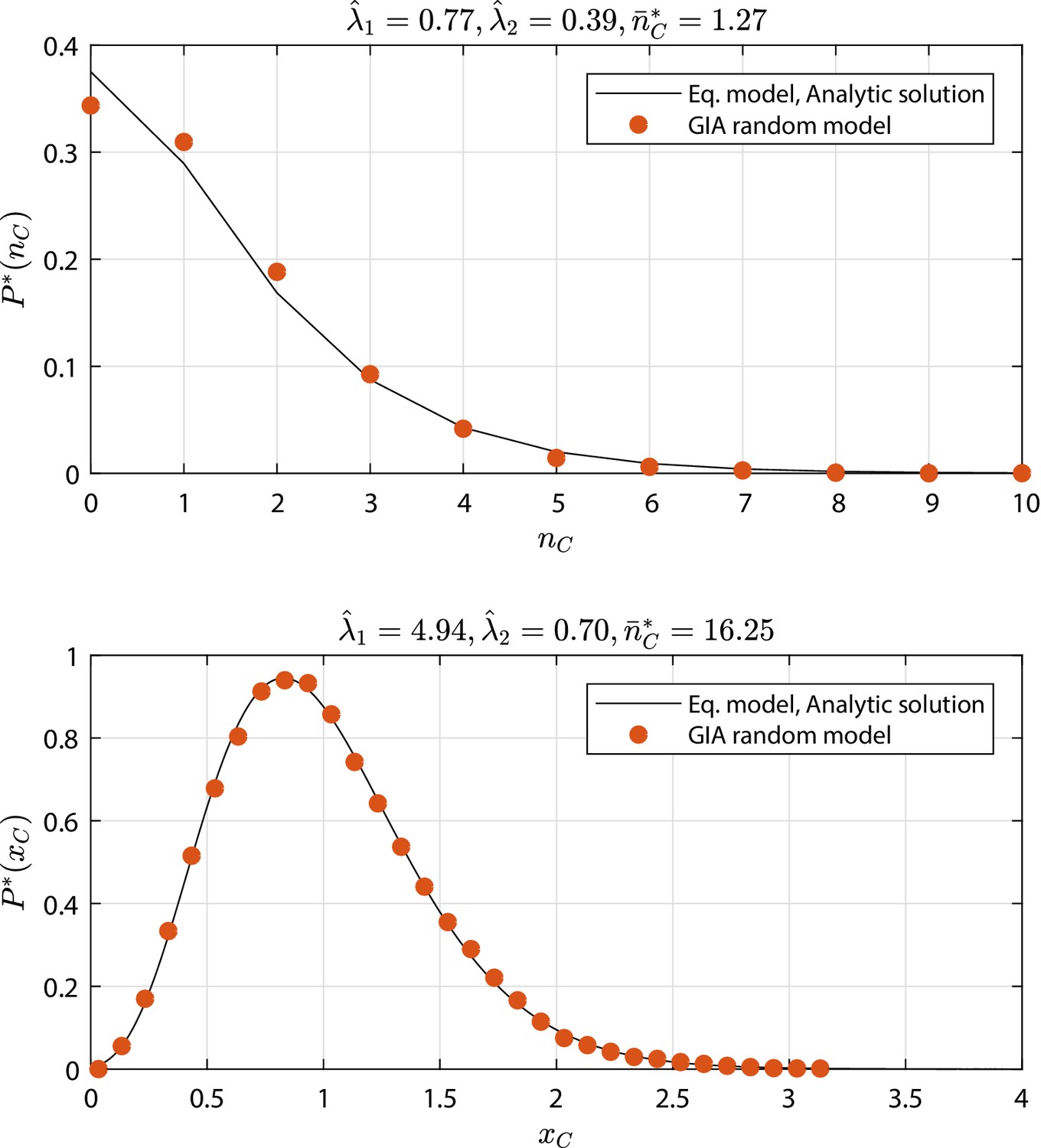
GIA random models selected cases (see Appendix 1—figure 9 and Appendix 1—figure 10) where $0.2 < {\hat{λ}}_{2} < 0.8$ : the steady state distribution $P^{*} (n_{C})$ (or the rescaled distribution $P^{*} (x_{C})$ ) of the number of cells in the committed compartment, $n_{C}$ (or in the rescaled case $x_{C} = n_{C} / {\bar{n}}_{C}^{*}$ ), is compared to that of the equivalent model (Equation model in the legend) analytic solution.

Results discussion is reported in 'Approximation of generic GIA models'.

Appendix 1—figure 14

Download asset Open asset

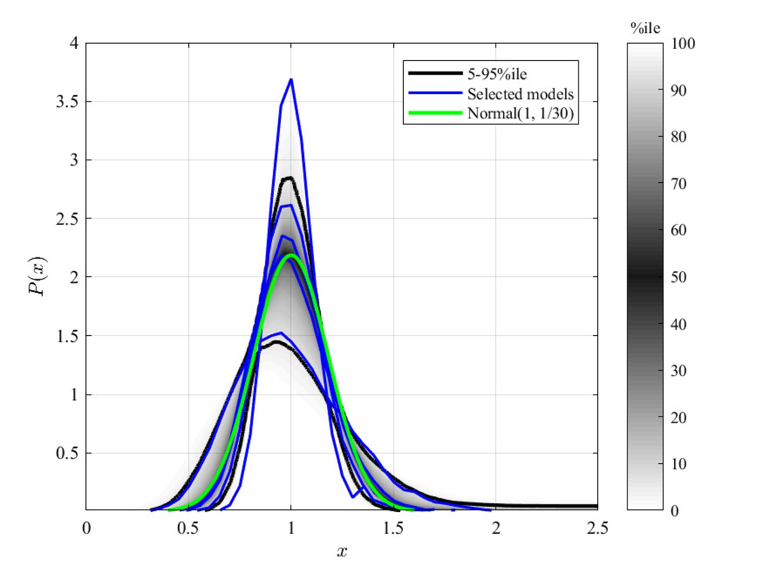
Rescaled clone size distribution for the random GIA models when ${\hat{λ}}_{R} = 30$ at the final simulation time, which corresponds to $20 / α_{\min}$ ( $α_{\min}$ is the minimum process rate).

The grey shade represents the percentile of all the simulations (black lines limit the 5-95%ile range); the blue curves correspond to some illustrative selected simulations. A reference curve corresponding to a Normal distribution of unitary mean and variance equal to $1 / {\hat{λ}}_{R} = 1 / 30$ is shown in green. Distributions of the total number of cells $n$ are scaled by the mean number of cells $\bar{n}$ , being $x = n / \bar{n}$ . Simulations for which the final condition (20 times the inverse of the minimum process rate) is not achieved (due to computational limitations) are not included, resulting in 922 models. Results discussion in provided in 'GIA model for large'.

Appendix 1—figure 15

Download asset Open asset

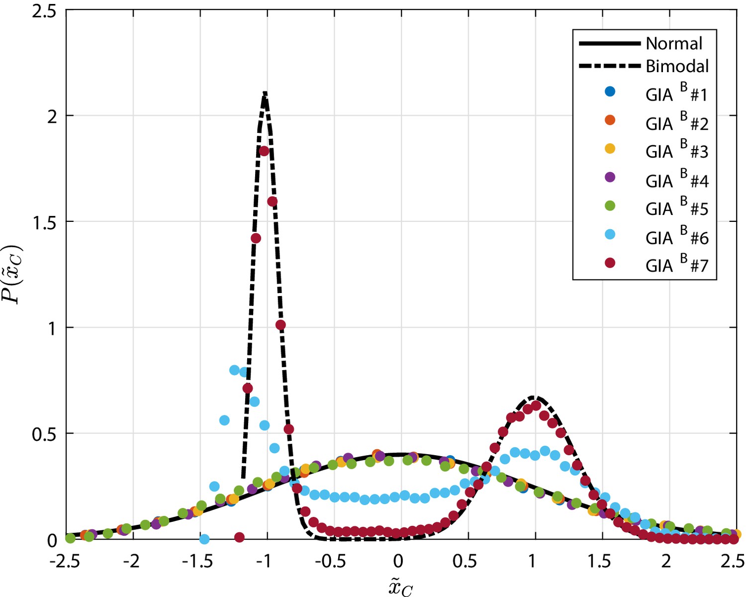
Rescaled distribution of the cells number in the committed compartment in the $G I A^{B}$ test cases at time τ, which is $20 / α_{\min}$ ( $α_{\min}$ is the minimum process rate).

The distributions $P ({\tilde{x}}_{C})$ of the number of cells in the committed compartment $n_{C}$ is rescaled considering that ${\tilde{x}}_{c} = (n_{C} - {\bar{n}}_{C}) / σ_{n_{c}}$ , where $σ_{n_{c}}$ is the variance of $n_{c}$ . In addition to the stochastic simulation results for different settings (see Appendix 1—table 2), the reference Normal and bimodal distributions are also shown. Results discussion is provided in 'GIA^B test case: bimodal distribution'.

Appendix 1—figure 16

Download asset Open asset

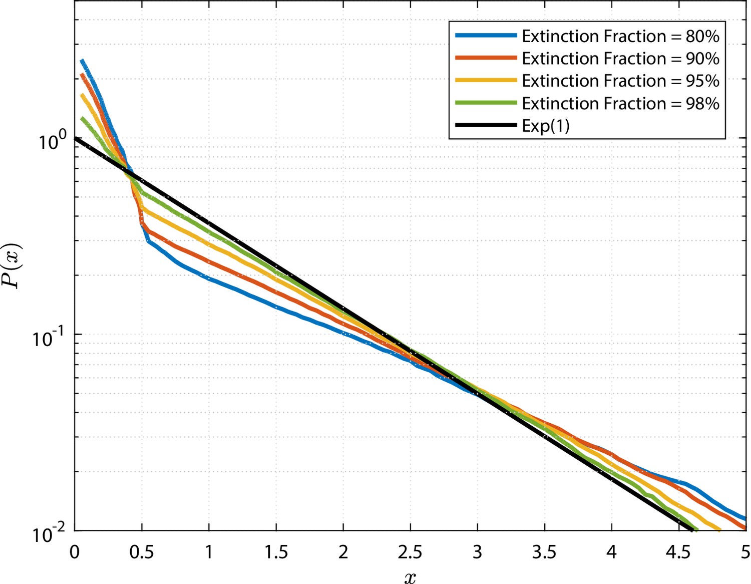
Clonal size distribution (corresponding to the 50%ile curve) in the GPA random models at different extinction fraction (i.e. different time).

The curves are compared to the expected Exponential distribution (see 'Analysis of the generalized Population Asymmetry model').

Tables

Appendix 1—table 1

IA and PA test cases simulation parameters (see 'Invariant Asymmetry and Population Asymmetry models').

Case	λ	γ	r
IA#1	1.0	1.0	-
IA#2	2.0	1.0	-
IA#3	5.0	1.0	-
PA#1	1.0	1.0	1/4
PA#2	2.0	1.0	1/4
PA#3	2.0	1.0	1/6

Appendix 1—table 2

GIA^B test case simulation parameters (see 'GIA^B test case: bimodal distribution').

Case	$\hat{ω}$	$λ_{1} / λ_{2}$
GIA^B#1	3 10¹	1
GIA^B#2	3 10^-2	1
GIA^B#3	3 10²	10
GIA^B#4	3 10¹	10
GIA^B#5	3 10⁰	10
GIA^B#6	3 10^-1	10
GIA^B#7	3 10^-2	10

Additional files

Transparent reporting form: https://cdn.elifesciences.org/articles/56532/elife-56532-transrepform-v2.docx
Download elife-56532-transrepform-v2.docx

Download links

A two-part list of links to download the article, or parts of the article, in various formats.

Downloads (link to download the article as PDF)

Article PDF

Open citations (links to open the citations from this article in various online reference manager services)

Mendeley

Cite this article (links to download the citations from this article in formats compatible with various reference manager tools)

Cristina Parigini
Philip Greulich

(2020)

Universality of clonal dynamics poses fundamental limits to identify stem cell self-renewal strategies

eLife 9:e56532.

https://doi.org/10.7554/eLife.56532

Figures

Illustration of the decomposition of a homeostatic cell state network into SCCs and the compartment representation, Equation 9.

Mean size of surviving clones, ${\bar{n}}_{s}$ , as a function of time for random GIA models (a), and GPA models (b).

Rescaled clone size distributions (expected relative frequency $P$ of clone sizes) for random GIA models (a), and GPA models (b), in terms of the rescaled clone size $x = n / {\bar{n}}_{s}$ , at final time $t = τ$ (see Figure 2 for definition).

Rescaled clone size distributions (expected relative frequency P of clone sizes) for random GIA models as in Figure 3, at time $t = τ$ (see definition in Figure 2).

Invariant Asymmetry (IA) test cases clone size distribution $P (n)$ , that is the distribution of the total number of cells n forming the progeny of a single initial cell in $ℛ$ .

Population Asymmetry (PA) test cases clone size distribution $P (n)$ , that is the distribution of the total number of cells n forming the progeny of a single initial stem cell.

Metastate (MS) test cases simulation results in terms of mean number of cells in the surviving clones ${\bar{n}}_{s}$ and extinction probability $P (n = 0)$ as function of time (scaled by the final simulation time τ).

Metastate (MS) test cases simulation results in terms clone size distribution $P (n)$ , that is the distribution of the total number of cells n forming the progeny of a single initial stem cell.

GIA⁰ test case parameters ${\hat{λ}}_{1}$ and ${\hat{λ}}_{2}$ over the contour map of the expected steady state mean number of cells in state $X_{2}$ , ${\bar{n}}_{2}^{*}$ .

GIA⁰ test case (see GIA⁰ test case: steady state distribution and limiting behavior') results in terms of steady state distribution $P^{*} (n_{2})$ of the the number of cells in state $X_{2}$ , $n_{2}$ .

GIA⁰ test case (see 'GIA⁰ test case: steady state distribution and limiting behavior') results in terms of steady state rescaled distribution $P^{} (x_{2})$ of the the number of cells in state $X_{2}$ , where $x_{2} = n_{2} / {\bar{n}}_{2}^{}$ .

GIA⁰ test case (see 'GIA⁰ test case: steady state distribution and limiting behavior') results in terms of steady state rescaled distribution $P^{} (x_{2})$ of the the number of cells in state $X_{2}$ , where $x_{2} = n_{2} / {\bar{n}}_{2}^{}$ .

Relative error of the the equivalent model approximation, $ϵ$ , (see definition in 'Approximation of generic GIA models') as function of ${\hat{λ}}_{2} = {\hat{λ}}_{C}$ for the GIA random models (generated as described in 'Generation of random models' and analyzed in the main text).

Rescaled clone size distribution for the random GIA models when ${\hat{λ}}_{R} = 30$ at the final simulation time, which corresponds to $20 / α_{\min}$ ( $α_{\min}$ is the minimum process rate).

Rescaled distribution of the cells number in the committed compartment in the $G I A^{B}$ test cases at time τ, which is $20 / α_{\min}$ ( $α_{\min}$ is the minimum process rate).

Clonal size distribution (corresponding to the 50%ile curve) in the GPA random models at different extinction fraction (i.e. different time).

Tables

IA and PA test cases simulation parameters (see 'Invariant Asymmetry and Population Asymmetry models').

GIA^B test case simulation parameters (see 'GIA^B test case: bimodal distribution').

Additional files

Transparent reporting form

Download links

Downloads (link to download the article as PDF)

Open citations (links to open the citations from this article in various online reference manager services)

Cite this article (links to download the citations from this article in formats compatible with various reference manager tools)

Be the first to read new articles from eLife

Share this article

Cite this article

Illustration of the decomposition of a homeostatic cell state network into SCCs and the compartment representation, Equation 9.

Mean size of surviving clones, n¯s, as a function of time for random GIA models (a), and GPA models (b).

Rescaled clone size distributions (expected relative frequency P of clone sizes) for random GIA models (a), and GPA models (b), in terms of the rescaled clone size x=n/n¯s, at final time t=τ (see Figure 2 for definition).

Rescaled clone size distributions (expected relative frequency P of clone sizes) for random GIA models as in Figure 3, at time t=τ (see definition in Figure 2).

Invariant Asymmetry (IA) test cases clone size distribution P⁢(n), that is the distribution of the total number of cells n forming the progeny of a single initial cell in ℛ.

Population Asymmetry (PA) test cases clone size distribution P⁢(n), that is the distribution of the total number of cells n forming the progeny of a single initial stem cell.

Metastate (MS) test cases simulation results in terms of mean number of cells in the surviving clones n¯s and extinction probability P(n=0) as function of time (scaled by the final simulation time τ).

Metastate (MS) test cases simulation results in terms clone size distribution P⁢(n), that is the distribution of the total number of cells n forming the progeny of a single initial stem cell.

GIA0 test case parameters λ^1 and λ^2 over the contour map of the expected steady state mean number of cells in state X2, n¯2*.

GIA0 test case (see GIA0 test case: steady state distribution and limiting behavior') results in terms of steady state distribution P*⁢(n2) of the the number of cells in state X2, n2.

GIA0 test case (see 'GIA0 test case: steady state distribution and limiting behavior') results in terms of steady state rescaled distribution P*⁢(x2) of the the number of cells in state X2, where x2=n2/n¯2*.

GIA0 test case (see 'GIA0 test case: steady state distribution and limiting behavior') results in terms of steady state rescaled distribution P*⁢(x2) of the the number of cells in state X2, where x2=n2/n¯2*.

Relative error of the the equivalent model approximation, ϵ, (see definition in 'Approximation of generic GIA models') as function of λ^2=λ^C for the GIA random models (generated as described in 'Generation of random models' and analyzed in the main text).

Rescaled clone size distribution for the random GIA models when λ^R=30 at the final simulation time, which corresponds to 20/αmin (αmin is the minimum process rate).

Rescaled distribution of the cells number in the committed compartment in the G⁢I⁢AB test cases at time τ, which is 20/αmin (αmin is the minimum process rate).

Clonal size distribution (corresponding to the 50%ile curve) in the GPA random models at different extinction fraction (i.e. different time).

IA and PA test cases simulation parameters (see 'Invariant Asymmetry and Population Asymmetry models').

GIAB test case simulation parameters (see 'GIAB test case: bimodal distribution').

Transparent reporting form

Downloads (link to download the article as PDF)

Open citations (links to open the citations from this article in various online reference manager services)

Cite this article (links to download the citations from this article in formats compatible with various reference manager tools)

Mean size of surviving clones, ${\bar{n}}_{s}$ , as a function of time for random GIA models (a), and GPA models (b).

Rescaled clone size distributions (expected relative frequency $P$ of clone sizes) for random GIA models (a), and GPA models (b), in terms of the rescaled clone size $x = n / {\bar{n}}_{s}$ , at final time $t = τ$ (see Figure 2 for definition).

Rescaled clone size distributions (expected relative frequency P of clone sizes) for random GIA models as in Figure 3, at time $t = τ$ (see definition in Figure 2).

Invariant Asymmetry (IA) test cases clone size distribution $P (n)$ , that is the distribution of the total number of cells n forming the progeny of a single initial cell in $ℛ$ .

Population Asymmetry (PA) test cases clone size distribution $P (n)$ , that is the distribution of the total number of cells n forming the progeny of a single initial stem cell.

Metastate (MS) test cases simulation results in terms of mean number of cells in the surviving clones ${\bar{n}}_{s}$ and extinction probability $P (n = 0)$ as function of time (scaled by the final simulation time τ).

Metastate (MS) test cases simulation results in terms clone size distribution $P (n)$ , that is the distribution of the total number of cells n forming the progeny of a single initial stem cell.

GIA⁰ test case parameters ${\hat{λ}}_{1}$ and ${\hat{λ}}_{2}$ over the contour map of the expected steady state mean number of cells in state $X_{2}$ , ${\bar{n}}_{2}^{*}$ .

GIA⁰ test case (see GIA⁰ test case: steady state distribution and limiting behavior') results in terms of steady state distribution $P^{*} (n_{2})$ of the the number of cells in state $X_{2}$ , $n_{2}$ .

GIA⁰ test case (see 'GIA⁰ test case: steady state distribution and limiting behavior') results in terms of steady state rescaled distribution $P^{} (x_{2})$ of the the number of cells in state $X_{2}$ , where $x_{2} = n_{2} / {\bar{n}}_{2}^{}$ .

GIA⁰ test case (see 'GIA⁰ test case: steady state distribution and limiting behavior') results in terms of steady state rescaled distribution $P^{} (x_{2})$ of the the number of cells in state $X_{2}$ , where $x_{2} = n_{2} / {\bar{n}}_{2}^{}$ .

Relative error of the the equivalent model approximation, $ϵ$ , (see definition in 'Approximation of generic GIA models') as function of ${\hat{λ}}_{2} = {\hat{λ}}_{C}$ for the GIA random models (generated as described in 'Generation of random models' and analyzed in the main text).

Rescaled clone size distribution for the random GIA models when ${\hat{λ}}_{R} = 30$ at the final simulation time, which corresponds to $20 / α_{\min}$ ( $α_{\min}$ is the minimum process rate).

Rescaled distribution of the cells number in the committed compartment in the $G I A^{B}$ test cases at time τ, which is $20 / α_{\min}$ ( $α_{\min}$ is the minimum process rate).

GIA^B test case simulation parameters (see 'GIA^B test case: bimodal distribution').