Short Report

Epidemiology and Global Health

Early analysis of the Australian COVID-19 epidemic

Centre for Epidemiology and Biostatistics, Melbourne School of Population and Global Health, The University of Melbourne, Australia
Victorian Infectious Diseases Reference Laboratory Epidemiology Unit at The Peter Doherty Institute for Infection and Immunity, The University of Melbourne and Royal Melbourne Hospital, Australia
Australian Institute of Tropical Health and Medicine, James Cook University, Australia
Telethon Kids Institute and Curtin University, Australia
Defence Science and Technology, Department of Defence, Australia
Kirby Institute for Infection and Immunity, University of New South Wales, Australia
School of Mathematics and Statistics, University of New South Wales, Australia
School of Public Health and Community Medicine, University of New South Wales, Australia
Centre for the Mathematical Modelling of Infectious Diseases, Department of Infectious Disease Epidemiology, London School of Hygiene and Tropical Medicine, United Kingdom
Infection and Immunity Theme, Murdoch Children’s Research Institute, The Royal Children’s Hospital, Australia
School of Mathematics and Statistics, The University of Melbourne, Australia

Aug 13, 2020

https://doi.org/10.7554/eLife.58785

Version of Record

Accepted for publication after peer review and revision.

Download
Cite
Share
CommentOpen annotations (there are currently 0 annotations on this page).

Version of Record published: August 26, 2020 (This version)
Accepted Manuscript published: August 13, 2020 (Go to version)
Accepted: August 12, 2020
Received: May 11, 2020

1. Part of Collection
COVID-19: A Collection of Articles

Edited by Diane M Harper et al.
Further reading

Abstract
Introduction
Materials and methods
Data availability
References
Decision letter
Author response
Article and author information
Metrics

Abstract

As of 1 May 2020, there had been 6808 confirmed cases of COVID-19 in Australia. Of these, 98 had died from the disease. The epidemic had been in decline since mid-March, with 308 cases confirmed nationally since 14 April. This suggests that the collective actions of the Australian public and government authorities in response to COVID-19 were sufficiently early and assiduous to avert a public health crisis – for now. Analysing factors that contribute to individual country experiences of COVID-19, such as the intensity and timing of public health interventions, will assist in the next stage of response planning globally. We describe how the epidemic and public health response unfolded in Australia up to 13 April. We estimate that the effective reproduction number was likely below one in each Australian state since mid-March and forecast that clinical demand would remain below capacity thresholds over the forecast period (from mid-to-late April).

Introduction

A small cluster of cases of the disease now known as COVID-19 was first reported on December 29, 2019, in the Chinese city of Wuhan (World Health Organization, 2020a). By early May 2020, the disease had spread to all global regions, and overwhelmed some the world’s most developed health systems. More than 2.8 million cases and 260,000 deaths had been confirmed globally, and the vast majority of countries with confirmed cases were reporting escalating transmission (World Health Organization, 2020b).

As of 1 May 2020, there were 6808 confirmed cases of COVID-19 in Australia. Of these, 98 had died from the disease. Encouragingly, the daily count of new confirmed cases had been declining since late March 2020, with 308 cases reported nationally since 14 April (Australian Government Department of Health, 2020a). This suggests that Australia has (to date) avoided a “worst-case” scenario — one where planning models estimated a peak daily demand for 35,000 ICU beds by around May 2020, far exceeding the health system’s capacity of around 2,200 ICU beds (Moss et al., 2020).

The first wave of COVID-19 epidemics, and the government and public responses to them, have varied vastly across the globe. For example, many European countries and the United States are in the midst of explosive outbreaks with overwhelmed health systems (Remuzzi and Remuzzi, 2020; The Lancet, 2020). Meanwhile, countries such as Singapore and South Korea had early success in containing the spread, partly attributed to their extensive surveillance efforts and case targeted interventions (Ng et al., 2020; COVID-19 National Emergency Response Center, Epidemiology and Case Management Team, Korea Centers for Disease Control and Prevention, 2020). However, despite those early successes, Singapore has recently taken additional steps to further limit transmission in the face of increasing importations and community spread (Government of Singapore, 2020). Other locations in the region, including Taiwan, Hong Kong and New Zealand, have had similar epidemic experiences, achieving control through a combination of border, case targeted and social distancing measures.

Analysing key epidemiological and response factors — such as the intensity and timing of public health interventions — that contribute to individual country experiences of COVID-19 will assist in the next stage of response planning globally.

Here we describe the course of the COVID-19 epidemic and public health response in Australia from 22 January up to mid-April 2020 (summarised in Figure 1). We then quantify the impact of the public health response on disease transmission (Figure 2) and forecast the short-term health system demand from COVID-19 patients (Figure 3).

Figure 1 with 2 supplements see all

Download asset Open asset

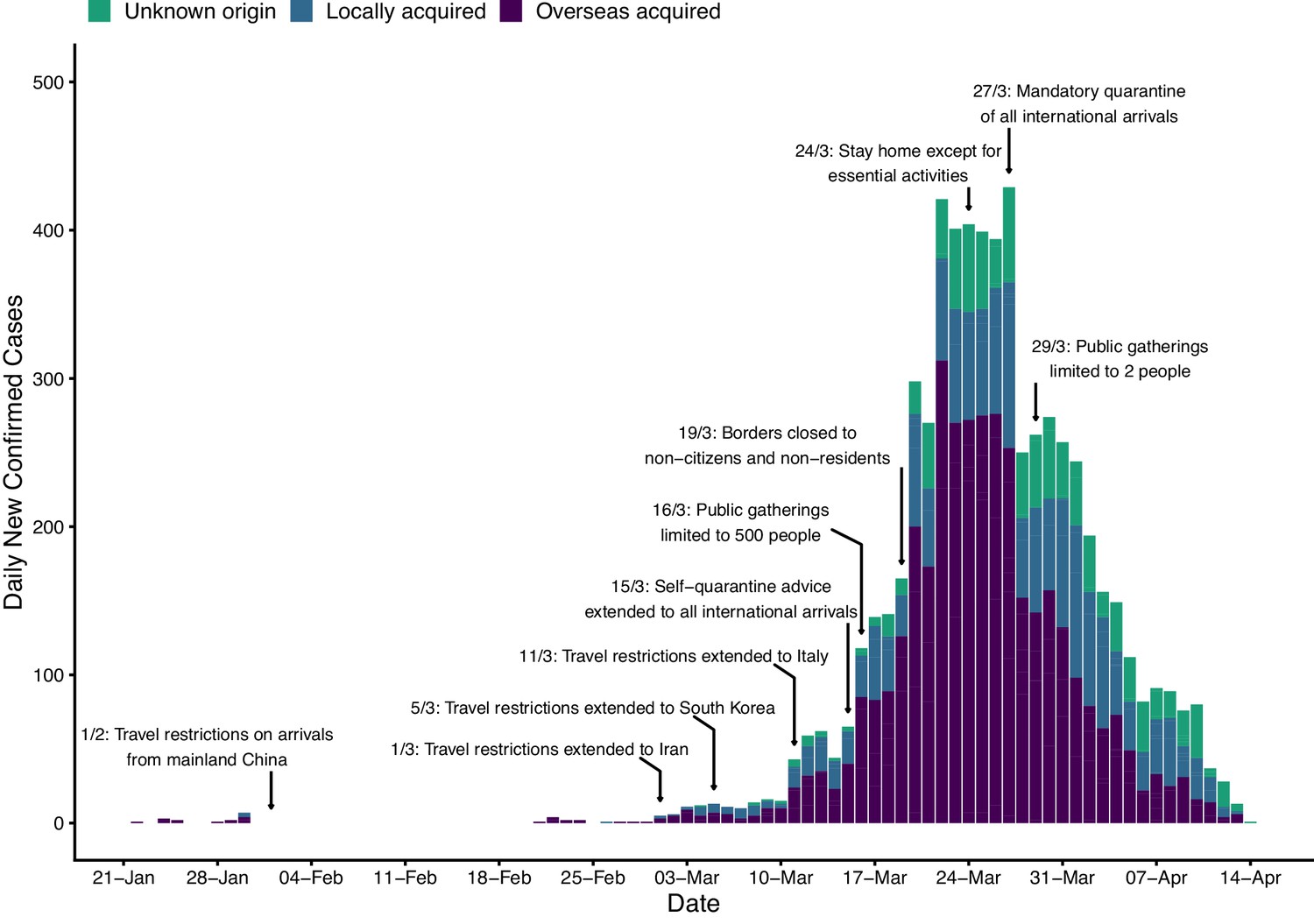
Time series of new daily confirmed cases of COVID-19 in Australia by import status (purple = overseas acquired, blue = locally acquired, green = unknown origin) from 22 January 2020 (first case detected) to 13 April 2020.

Dates of selected key border and social distancing measures implemented by Australian authorities are indicated by annotations above the plotted case counts. These measures were in addition to case targeted interventions (case isolation and contact quarantine) and further border measures, including enhanced testing and provision of advice, on arrivals from other selected countries, based on a risk-assessment tool developed in early February (Shearer et al., 2020). Note that Australian citizens and residents (and their dependants) were exempt from travel restrictions, but upon returning to Australia were required to quarantine for 14 days from the date of arrival. A full timeline of social distancing and border measures is provided in Figure 1—figure supplement 2.

Figure 2 with 3 supplements see all

Download asset Open asset

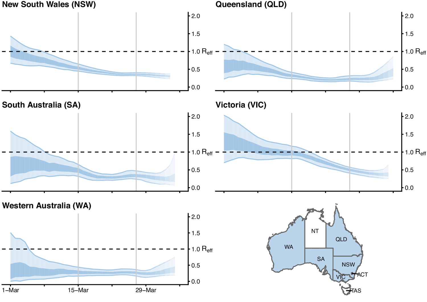
Time-varying estimate of the effective reproduction number ( $R_{𝑒𝑓𝑓}$ ) of COVID-19 by Australian state (light blue ribbon = 90% credible interval; dark blue ribbon = 50% credible interval) from 1 March to 5 April 2020, based on data up to and including 13 April 2020.

Confidence in the estimated values is indicated by shading with reduced shading corresponding to reduced confidence. The horizontal dashed line indicates the target value of 1 for the effective reproduction number required for control. Not presented are the Australian Capital Territory (ACT), Northern Territory (NT) and Tasmania (TAS), as these states/territories had insufficient local transmission. The uncertainty in the $R_{𝑒𝑓𝑓}$ estimates represent variability in a population-level average as a result of imperfect data, rather than individual-level heterogeneity in transmission (*i.e.*, the variation in the number of secondary cases generated by each case).

Figure 3 with 1 supplement see all

Download asset Open asset

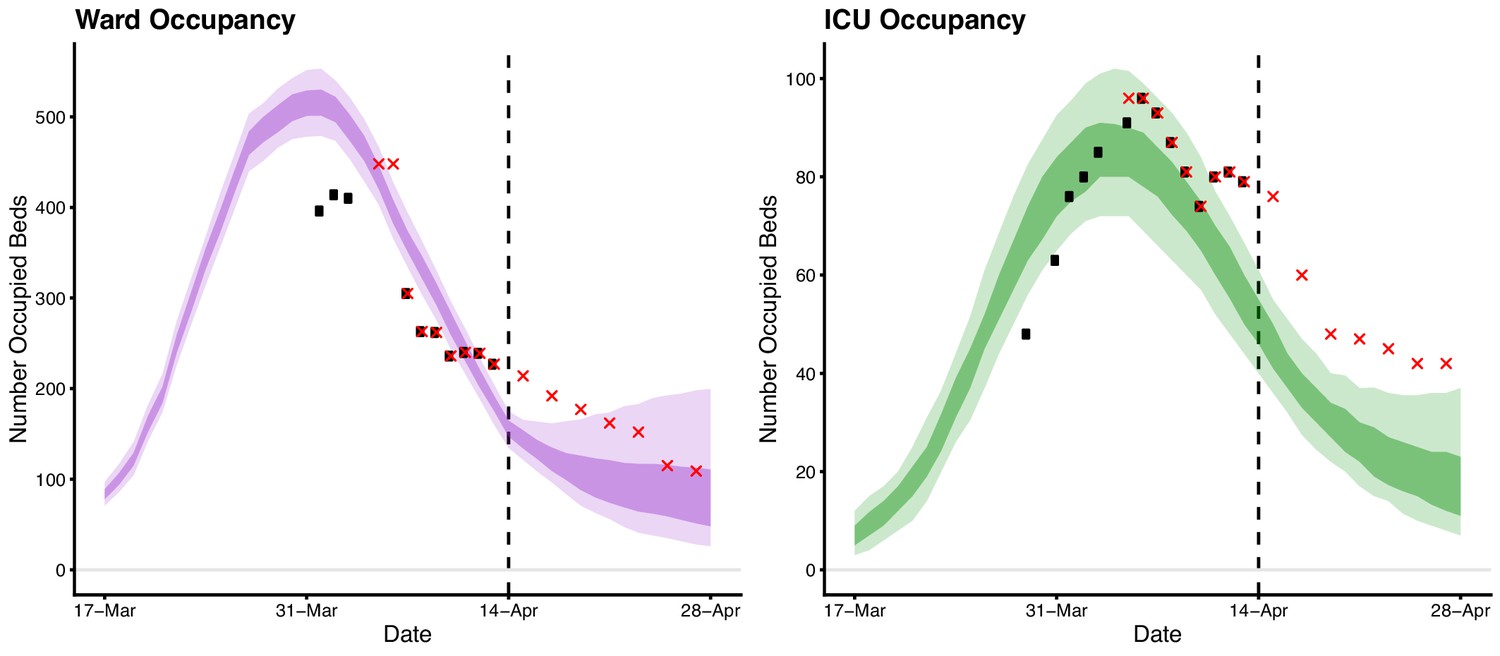
Forecasted daily hospital ward (left) and intensive care unit (right) occupancy (dark ribbons = 50% confidence intervals; light ribbons = 95% confidence intervals) from 17 March to 28 April.

Occupancy = the number of beds occupied by COVID-19 patients on a given day. Black dots indicate the reported ward and ICU occupancy available from the Australian national COVID-19 database at the time. These data were retrospectively updated where complete data were available (red crosses). Australian health system ward and ICU bed capacities are estimated to be over 25,000 and 1,100, respectively, under the assumption that 50% of total capacity could possibly be dedicated to COVID-19 patients (Australian Institute of Health and Welfare, 2019). The forecasted daily case counts are shown in Figure 3—figure supplement 1.

Timeline of the Australian epidemic

Australia took an early and precautionary approach to COVID-19. On 1 February, when China was the only country reporting uncontained transmission, Australian authorities restricted all travel from mainland China to Australia, in order to reduce the risk of importation of the virus. Only Australian citizens and residents (and their dependants) were permitted to travel from China to Australia. These individuals were advised to self-quarantine for 14 days from their date of arrival. Further border measures, including enhanced testing and provision of additional advice, were placed on arrivals from other countries, based on a risk-assessment tool developed in early February (Shearer et al., 2020).

The day before Australia imposed these restrictions (January 31), 9720 cases of COVID-19 had been reported in mainland China (World Health Organization, 2020c). Australia had so far detected and managed nine imported cases, all with recent travel history from or a direct epidemiological link to Wuhan (Australian Government Department of Health, 2020b). Before the restrictions, Australia was expecting to receive approximately 200,000 air passengers from mainland China during February 2020 (Australian Bureau of Statistics, 2019). Travel numbers fell dramatically following the imposed travel restrictions.

These restrictions were not intended (and highly unlikely [Errett et al., 2020]) to prevent the ultimate importation of COVID-19 into Australia. Their purpose was to delay the establishment of an epidemic, buying valuable time for health authorities to plan and prepare.

During the month of February, with extensive testing and case targeted interventions (case isolation and contact quarantine) initiated from 29 January (Australian Government Department of Health, 2020d), Australia detected and managed only 12 cases. Meanwhile, globally, the geographic extent of transmission and daily counts of confirmed cases and deaths continued to increase drastically (World Health Organization, 2020d). In early March, Australia extended travel restrictions to a number of countries with large uncontained outbreaks, namely Iran (as of 1 March) (Commonwealth Government of Australia, 2020a), South Korea (as of 5 March) (Commonwealth Government of Australia, 2020b) and Italy (as of 11 March) (Commonwealth Government of Australia, 2020c).

Despite these measures, the daily case counts rose sharply in Australia during the first half of March. While the vast majority of these cases were connected to travellers returning to Australia from overseas, localised community transmission had been reported in areas of Sydney (NSW) and Melbourne (VIC) (Australian Government Department of Health, 2020c). Crude plots of the cumulative number of cases by country showed Australia on an early trajectory similar to the outbreaks experienced in China, Europe and the United States, where health systems had become or were becoming overwhelmed (Australian Government Department of Health, 2020f).

From 16 March, the Australian Government progressively implemented a range of social distancing measures in order to reduce and prevent further community transmission (Commonwealth Government of Australia, 2020d). The day before, authorities had imposed a self-quarantine requirement on all international arrivals (Commonwealth Government of Australia, 2020e). On 19 March, Australia closed its borders to all non-citizens and non-residents (Commonwealth Government of Australia, 2020f), and on March 27, moved to a policy of mandatory quarantine for any returning citizens and residents (Commonwealth Government of Australia, 2020g). By 29 March, social distancing measures had been escalated to the extent that all Australians were strongly advised to leave their homes only for limited essential activities and public gatherings were limited to two people (Commonwealth Government of Australia, 2020h).

By late March, daily counts of new cases appeared to be declining, suggesting that these measures had successfully reduced transmission.

Quantifying the impact of the response

Quantifying changes in the rate of spread of infection over the course of an epidemic is critical for monitoring the collective impact of public health interventions and forecasting the short-term clinical burden. A key indicator of transmission in context is the effective reproduction number ( $R_{𝑒𝑓𝑓}$ ) — the average number of secondary infections caused by an infected individual in the presence of public health interventions and for which no assumption of 100% susceptibility is made. If control efforts are able to bring $R_{𝑒𝑓𝑓}$ below 1, then on average there will be a decline in the number of new cases reported. The decline will become apparent after a delay of approximately one incubation period plus time to case detection and reporting following implementation of the control measure (i.e., at least two weeks).

Using case counts from the Australian national COVID-19 database, we estimated $R_{𝑒𝑓𝑓}$ over time for each Australian state from 24 February to 5 April 2020 (Figure 2). We used a statistical method that estimates time-varying $R_{𝑒𝑓𝑓}$ by using an optimally selected moving average window (according to the continuous ranked probability score) to smooth the curve and reduce the impact of localised clusters and outbreaks that may cause large fluctuations (London School of Hygiene & Tropical Medicine Mathematical Modelling of Infectious Diseases nCoV working group, 2020). Importantly, the method accounts for time delays between illness onset and case notification. Incorporation of this lag is critical for accurate interpretation of the most recent data in the analysis, to be sure that an observed drop in the number of reported cases reflects an actual drop in case numbers.

Results show that $R_{𝑒𝑓𝑓}$ has likely been below one in each Australian state since early-to-mid March. These estimates are geographically averaged results over large areas and it is possible that $R_{𝑒𝑓𝑓}$ was much higher than one in a number of localised settings (see Figure 2). The estimated time-varying $R_{𝑒𝑓𝑓}$ value is based on cases that have been identified as a result of local transmission, whereas imported cases only contribute to the force of infection. Imported and locally acquired cases were assumed to be equally infectious. The method for estimating $R_{𝑒𝑓𝑓}$ is sensitive to this assumption. Hence, we performed a sensitivity analysis to assess the impact of stepwise reductions in the infectiousness of imported cases on $R_{𝑒𝑓𝑓}$ as a result of quarantine measures implemented over time (see Figure 2—figure supplement 1, Figure 2—figure supplement 2, and Figure 2—figure supplement 3). The sensitivity analyses suggest that $R_{𝑒𝑓𝑓}$ may well have dropped below one later than shown in Figure 2.

In Victoria and New South Wales, the two Australian states with a substantial number of local cases, the effective reproduction number likely dropped from marginally above one to well below one within a two week period (considering both our main result and those from the sensitivity analyses) coinciding with the implementation of social distancing measures. A comparable trend was observed in New Zealand and many Western European countries, including France, Spain and Germany (London School of Hygiene & Tropical Medicine Mathematical Modelling of Infectious Diseases nCoV working group, 2020), where similar national, stage-wise social distancing policies were enacted (Flaxman et al., 2020). However, most of these European countries experienced widespread community transmission prior to the implementation of social distancing measures, with $R_{𝑒𝑓𝑓}$ estimates reaching between 1.5 and 2 in early March and declining over a longer period (three to four weeks) relative to Australia.

Forecasting the clinical burden

Next we used our estimates of time-varying $R_{𝑒𝑓𝑓}$ to forecast the short-term clinical burden in Australia. Estimates were input into a mathematical model of disease dynamics that was extended to account for imported cases. A sequential Monte Carlo method was used to infer the model parameters and appropriately capture the uncertainty (Moss et al., 2019a), conditional on each of a number of sampled $R_{𝑒𝑓𝑓}$ trajectories up to 5 April, from which point they were assumed to be constant. The model was subsequently projected forward from April 14 to April 28, to forecast the number of reported cases, assuming a symptomatic detection probability of 80%.

The number of new daily hospitalisations and ICU admissions were estimated from recently observed and forecast case counts. Specifically, the age distribution of projected cases, and age-specific probabilities of hospitalisation and ICU admission, were extracted from Australian age-specific data on confirmed cases, assuming that this distribution would remain unchanged (see Table 1). In order to calculate the number of occupied ward/ICU beds per day, length-of-stay in a ward bed and ICU bed were assumed to be Gamma distributed with means (SD) of 11 (3.42) days and 14 (5.22) days, respectively. Our results indicated that with the public health interventions in place as of 13 April, Australia’s hospital ward and ICU occupancy would remain well below capacity thresholds over the period from 14 to 28 April.

Table 1

Age-specific proportions of confirmed cases extracted from the Australian national COVID-19 database and age-specific estimates of the probability of hospitalisation and ICU admission for confirmed cases.

Age	Proportion of cases	Pr(hospitalisation \| confirmed case)	Pr(ICU admission \| confirmed case)
0-9	0.0102	0.1475	0.0000
10-18	0.0186	0.1081	0.0090
19-29	0.2258	0.0504	0.0007
30-39	0.1587	0.0865	0.0074
40-49	0.1291	0.0947	0.0208
50-59	0.1550	0.1112	0.0173
60-69	0.1686	0.1529	0.0318
70-79	0.1050	0.2440	0.0558
80+	0.0290	0.3815	0.0462

Conclusions

Our analysis suggests that Australia’s combined strategy of early, targeted management of the risk of importation, case targeted interventions, and broad-scale social distancing measures applied prior to the onset of (detected) widespread community transmission has substantially mitigated the first wave of COVID-19. More detailed analyses are required to assess the relative impact of specific response measures, and this information will be crucial for the next phase of response planning. Other factors, such as temperature, humidity and population density may influence transmission of SARS-CoV-2 (Kissler et al., 2020). Whether these factors have played a role in the relative control of SARS-CoV-2 in some countries, remains an open question. Noting that epidemics are established in both the northern and southern hemispheres, it may be possible to gain insight into such factors over the next six months, via for example a comparative analysis of transmission in Australia and Europe.

We further anticipated that the Australian health care system was well positioned to manage the projected COVID-19 case loads over the forecast period (up to 28 April). Ongoing situational assessment and monitoring of forecast hospital and ICU demand will be essential for managing possible future relaxation of broad-scale community interventions. Vigilance for localised increases in epidemic activity and in particular for outbreaks in vulnerable populations such as residential aged care facilities, where a high proportion of cases are likely to be severe, must be maintained.

One largely unknown factor at present is the proportion of SARS-CoV-2 infections that are asymptomatic, mild or undiagnosed. Even if this number is high, the Australian population would still be largely susceptible to infection. Accordingly, complete relaxation of the measures currently in place would see a rapid resurgence in epidemic activity. This problem is not unique to Australia. Many countries with intensive social distancing measures in place are starting to grapple with their options and time frames for a gradual return to relative normalcy (Gottlieb et al., 2020).

There are difficult decisions ahead for governments, and for now Australia is one of the few countries fortunate enough to be able to plan the next steps from a position of relative calm as opposed to crisis.

Materials and methods

Estimating the time-varying effective reproduction number

Overview

The method used to estimate $R_{𝑒𝑓𝑓}$ is described in Cori et al., 2013, as implemented in the R package, EpiNow (Abbott et al., 2020). This method is currently in development by the Centre for the Mathematical Modelling of Infectious Diseases at the London School of Hygiene and Tropical Medicine (London School of Hygiene & Tropical Medicine Mathematical Modelling of Infectious Diseases nCoV working group, 2020). Full details of their statistical analysis and code base is available via their website (https://epiforecasts.io/covid/).

The uncertainty in the $R_{𝑒𝑓𝑓}$ estimates (shown in Figure 2; Figure 2—figure supplements 1, 2 and 3) represents variability in a population-level average as a result of imperfect data, rather than individual-level heterogeneity in transmission (i.e., the variation in the number of secondary cases generated by each case). This is akin to the variation represented by a confidence interval (i.e., variation in the estimate resulting from a finite sample), rather than a prediction interval (i.e., variation in individual observations).

We provide a brief overview of the method and sources of imperfect data below, focusing on how the analysis was adapted to the Australian context.

Data

We used line-lists of reported cases for each Australian state/territory extracted from the national COVID-19 database. The line-lists contain the date when the individual first exhibited symptoms, date when the case notification was received by the jurisdictional health department and where the infection was acquired (i.e., overseas or locally).

Reporting delays and under-reporting

Request a detailed protocol

A pre-hoc statistical analysis was conducted in order to estimate a distribution of the reporting delays from the line-lists of cases, using the code base provided by London School of Hygiene & Tropical Medicine Mathematical Modelling of Infectious Diseases nCoV working group, 2020. The estimated reporting delay is assumed to remain constant over time. These reporting delays are used to: (i) infer the time of symptom onset for those without this information, and; (ii) infer how many cases in recent days are yet to be recorded. Adjusting for reporting delays is critical for inferring when a drop in observed cases reflects a true drop in cases.

Trends identified using this approach are robust to under-reporting, assuming that it is constant. However, absolute values of $R_{𝑒𝑓𝑓}$ may be biased by reporting rates. Pronounced changes in reporting rates may also impact the trends identified.

The delay from symptom onset to reporting is likely to decrease over the course of the epidemic, due to improved surveillance and reporting. We used a delay distribution estimated from observed reporting delays from the analysis period, which is therefore likely to underestimate reporting delays early in the epidemic, and overestimate them as the epidemic progressed. Underestimating the delay would result in an overestimate of $R_{𝑒𝑓𝑓}$ , as the inferred onset dates (for those that were unknown) and adjustment for right-truncation, would result in more concentrated inferred daily cases (i.e., the inferred cases would be more clustered in time than in reality). The converse would be true when overestimating the delay. The impact of this misspecified distribution will be greatest on the most recent estimates of $R_{𝑒𝑓𝑓}$ , where inference for both right-truncation and missing symptom onset dates is required.

Estimating the effective reproduction number over time

Request a detailed protocol

Briefly, the $R_{𝑒𝑓𝑓}$ was estimated for each day from 24 February 2020 up to 5 April 2020 using line list data – date of symptom onset, date of report, and import status – for each state. The method assumes that the serial interval (i.e., time between symptom onset for an index and secondary case) is uncertain, with a mean of 4.7 days (95% CrI: 3.7, 6.0) and a standard deviation of 2.9 days (95% CrI: 1.9, 4.9), as estimated from early outbreak data in Wuhan, China (Nishiura et al., 2020). Combining the incidence over time with the uncertain distribution of serial intervals allows us to estimate $R_{𝑒𝑓𝑓}$ over time.

A different choice of serial interval distribution would affect the estimated time varying $R_{𝑒𝑓𝑓}$ . This sensitivity is explored in detail in Flaxman et al., 2020, though we provide a brief description of the impact here. For the same daily case data, a longer average serial interval would correspond to an increased estimate of $R_{𝑒𝑓𝑓}$ when $R_{𝑒𝑓𝑓} > 1$ , and a decreased estimate when $R_{𝑒𝑓𝑓} < 1$ . This effect can be understood intuitively by considering the epidemic dynamics in these two situations. When $R_{𝑒𝑓𝑓} > 1$ , daily case counts are increasing on average. The weighted average case counts (weighted by the serial interval distribution), decrease as the mean of the serial interval increases (i.e., as the support is shifted to older/lower daily case data). In order to generate the same number of observed cases in the present, $R_{𝑒𝑓𝑓}$ must increase. A similar observation can be made for $R_{𝑒𝑓𝑓} < 1$ .

In the context of our analyses (Figure 2), when the estimated $R_{𝑒𝑓𝑓}$ is above 1, assuming a longer mean serial interval would further increase the $R_{𝑒𝑓𝑓}$ estimates in each jurisdiction (i.e., the upper 75% of the Victorian posterior distribution for approximately the first 7–10 days, while stretching the upper tails in the other jurisdictions). When the estimated $R_{𝑒𝑓𝑓}$ is below 1, a higher mean serial interval would further decrease those estimates. Qualitatively, this does not impact on the time series of $R_{𝑒𝑓𝑓}$ in each Australian jurisdiction.

A prior distribution was specified for $R_{𝑒𝑓𝑓}$ , with mean 2.6 (informed by Imai et al., 2020) and a broad standard deviation of 2 so as to allow for a range of $R_{𝑒𝑓𝑓}$ values. Finally, $R_{𝑒𝑓𝑓}$ is estimated with a moving average window, selected to optimise the continuous ranked probability score, in order to smooth the curve and reduce the impact of localised events (i.e., cases clustered in time) causing large variations.

Note that up to 20% of reported cases in the Australian national COVID-19 database do not have a reported import status (see Figure 1). Conservatively, we assumed that all cases with an unknown or unconfirmed source of acquisition were locally acquired.

Accounting for imported cases

Request a detailed protocol

A large proportion of cases reported in Australia from January until now were imported from overseas. It is critical to account for two distinct populations in the case notification data – imported and locally acquired – in order to perform robust analyses of transmission in the early stages of this outbreak. The estimated time-varying $R_{𝑒𝑓𝑓}$ value is based on cases that have been identified as a result of local transmission, whereas imported cases contribute to transmission only (Thompson et al., 2019).

Specifically, the method assumes that local and imported cases contribute equally to transmission. The results under this assumption are presented in Figure 2. However, it is likely that imported cases contributed relatively less to transmission than locally acquired cases, as a result of quarantine and other border measures which targeted these individuals (Figure 1—figure supplement 2). In the absence of data on whether the infector of local cases was themselves an imported or local case (from which we could robustly estimate the contribution of imported cases to transmission), we explored this via a sensitivity analysis. We aimed to explore the impact of a number of plausible scenarios, based on our knowledge of the timing, extent and level of enforcement of different quarantine policies enacted over time.

Prior to 15 March, returning Australian residents and citizens (and their dependents) from mainland China were advised to self-quarantine. Note that further border measures were implemented during this period, including enhanced testing and provision of advice on arrivals from selected countries based on a risk assessment tool developed in early February (Shearer et al., 2020). On 15 March, Australian authorities imposed a self-quarantine requirement on all international arrivals, and from 27 March, moved to a mandatory quarantine policy for all international arrivals.

Hence for the sensitivity analysis, we assumed two step changes in the effectiveness of quarantine of overseas arrivals (timed to coincide with the two key policy changes), resulting in three intervention phases: prior to 15 March (self-quarantine of arrivals from selected countries); 15–27 March inclusive (self-quarantine of arrivals from all countries); and 27 March onward (mandatory quarantine of overseas arrivals from all countries). We further assumed that the relative infectiousness of imported cases decreased with each intervention phase. The first two intervention phases correspond to self-quarantine policies, so we assume that they resulted in a relatively small reduction in the relative infectiousness of imported cases (the first smaller than the second, since the pre-15 March policy only applied to arrivals from selected countries). The third intervention phase corresponds to mandatory quarantine of overseas arrivals in hotels which we assume is highly effective at reducing onward transmission from imported cases, but allows for the occasional transmission event. We then varied the percentage of imported cases contributing to transmission over the three intervention phases, as detailed in Table 2.

Table 2

Percentage of imported cases assumed to be contributing to transmission over three intervention phases for each sensitivity analysis.

We assume two step changes in the effectiveness of quarantine of overseas arrivals, resulting in three intervention phases: prior to 15 March (self-quarantine of arrivals from selected countries); 15–27 March inclusive (self-quarantine of arrivals from all countries); and 27 March onward (mandatory quarantine of overseas arrivals from all countries).

	Imported cases contributing to transmission
Sensitivity analysis	Prior to 15 March	15–27 March	27 March–
1	90%	50%	1%
2	80%	50%	1%
3	50%	20%	1%

The results of these three analyses are shown in Figure 2—figure supplements 1, 2 and 3, respectively.

Forecasting short-term ward and ICU bed occupancy

We used the estimates of time-varying $R_{𝑒𝑓𝑓}$ to forecast the national short-term ward/ICU occupancy due to COVID-19 patients.

Forecasting case counts

Request a detailed protocol

The forecasting method combines an SEEIIR (susceptible-exposed-infectious-recovered) population model of infection with daily COVID-19 case notification counts, through the use of a bootstrap particle filter (Arulampalam et al., 2002). This approach is similar to that implemented and described in Moss et al., 2019b, in the context of seasonal influenza forecasts for several major Australian cities. Briefly, the particle filter method uses post-regularisation (Doucet et al., 2001), with a deterministic resampling stage (Kitagawa, 1996). Code and documentation are available at https://epifx.readthedocs.io/en/latest/. The daily case counts by date of diagnosis were modelled using a negative binomial distribution with a fixed dispersion parameter k, and the expected number of cases was proportional to the daily incidence of symptomatic infections in the SEEIIR model; this proportion was characterised by the observation probability. Natural disease history parameters were sampled from narrow uniform priors, based on values reported in the literature for COVID-19 (Table 3), and each particle was associated with an $R_{𝑒𝑓𝑓}$ trajectory that was drawn from the state/territory $R_{𝑒𝑓𝑓}$ trajectories in Figure 2 up to 5 April, from which point they are assumed to be constant. The model was subsequently projected forward from April 14 to April 28, to forecast the number of reported cases, assuming a detection probability of 80%.

Table 3

SEEIIR forecasting model parameters.

Parameter	Definition	Value/Prior distribution
σ	Inverse of the mean incubation period	$U (4^{- 1}, 3^{- 1})$
γ	Inverse of the mean infectious period	$U (10^{- 1}, 9^{- 1})$
τ	Time of first exposure (days since 2020-01-01)	$U (0, 28)$
$p_{𝑜𝑏𝑠}$	Probability of observing a case	0.8
k	Dispersion parameter on Negative-Binomial	100
	observation model

In order to account for imported cases, we used daily counts of imported cases to construct a time-series of the expected daily importation rate and, assuming that such cases were identified one week after initial exposure, introduced exposure events into each particle trajectory by adding an extra term to the force of infection equation.

Model equations below describe the flow of individuals in the population from the susceptible class (S), through two exposed classes (E₁, E₂), two infectious classes (I₁, I₂) and finally into a removed class (R). The state variables $S, E_{1}, E_{2}, I_{1}, I_{2}, R$ correspond to the proportion of individuals in the population (of size N) in each compartment. Given the closed population and unidirectional flow of individuals through the compartments, we evaluate the daily incidence of symptomatic individuals (at time t) as the change in cumulative incidence (the bracketed term in the expression for $𝔼 [y_{t}]$ below). Two exposed and infectious classes are chosen such that the duration of time in the exposed or infectious period has an Erlang distribution. The corresponding parameters are given in Table 2.

Model equations:

\begin{array}{ll} \frac{d S}{d t} & = - β (t) \cdot S (I_{1} + I_{2}) \\ \frac{d E_{1}}{d t} & = β (t) \cdot S (I_{1} + I_{2}) - 2 σ E_{1} \\ \frac{d E_{2}}{d t} & = 2 σ E_{1} - 2 σ E_{2} \\ \frac{d I_{1}}{d t} & = 2 σ E_{2} - 2 γ I_{1} \\ \frac{d I_{2}}{d t} & = 2 γ I_{1} - 2 γ I_{2} \\ \frac{d R}{d t} & = 2 γ I_{2} \end{array}

With initial conditions:

\begin{array}{ll} S (0) & = \frac{N - 10}{N} \\ E_{1} (0) & = \frac{10}{N} \\ E_{2} (0) & = I_{1} (0) = I_{2} (0) = R (0) = 0 \end{array}

Observation model:

\begin{array}{ll} E [y_{t}] & = N \cdot p_{o b s} \cdot [I_{2} (t) + R (t) - (I_{2} (t - 1) + R (t - 1))] \\ x_{t} & = [S (t), E_{1} (t), E_{2} (t), I_{1} (t), I_{2} (t), R (t), β^{i} (t), σ, γ, τ] \\ ℒ (y_{t} ∣ x_{t}) & \sim NegBin (E [y_{t}], k) \end{array}

With time-varying transmission rate corresponding to $R_{𝑒𝑓𝑓}$ trajectory i:

\begin{array}{ll} β^{i} (t) & = {\begin{cases} 0, & if t < τ \\ R_{e f f}^{i} (t) \cdot γ, & if t \geq τ, \end{cases} for i \in {1, 2, . . ., 10} \end{array}

Forecasting ward and ICU bed occupancy from observed and projected case counts

Request a detailed protocol

The number of new daily hospitalisations and ICU admissions were estimated from recently observed and forecasted case counts by:

Estimating the age distribution of projected case counts using data from the national COVID-19 database on the age-specific proportion of confirmed cases;
Estimating the age-specific hospitalisation and ICU admission rates using data from the national COVID-19 database. We assumed that all hospitalisations and ICU admissions were either recorded or were missing at random (31% and 58% of cases had no information recorded under hospitalisation or ICU status, respectively);
Randomly drawing the number of hospitalisations/ICU admissions in each age-group (for both the observed and projected case counts) from a binomial distribution with number of trials given by the expected number of cases in each age group (from 1), and probability given by the observed proportion of hospitalisations/ICU admissions by age group (from 2).

Finally, in order to calculate the number of occupied ward/ICU beds per day, length-of-stay in a ward bed and ICU bed were assumed to be Gamma distributed with means (SD) of 11 (3.42) days and 14 (5.22) days, respectively. We assumed ICU admissions required a ward bed prior to, and following, ICU stay for a Poisson distributed number of days with mean 2.5. Relevant Australian data were not available to parameterise a model that captures the dynamics of patient flow within the hospital system in more detail. Instead, these distributions were informed by a large study of clinical characteristics of 1099 COVID-19 patients in China (Guan et al., 2020). This model provides a useful indication of hospital bed occupancy based on limited available data and may be updated as more specific data (e.g., on COVID-19 patient length-of-stay) becomes available.

Data availability

Analysis code is included in the supplementary materials. Datasets analysed and generated during this study are included in the supplementary materials. For estimates of the time-varying effective reproduction number (Figure 2), the complete line listed data within the Australian national COVID-19 database are not publicly available. However, we provide the cases per day by notification date and state (as shown in Figure 1 and Figure 1–figure supplement 1) which, when supplemented with the estimated distribution of the delay from symptom onset to notification (samples from this distribution are provided as a data file), analyses of the time-varying effective reproduction number can be performed.

References

Software
1. Abbott S
2. Hellewell J
3. Munday J
4. Thompson R
5. Funk S
(2020) EpiNow: Estimate realtime case counts and time-varying epidemiological parameters, version 0.1.0
Github.

https://github.com/epiforecasts/EpiNow
(2002) A tutorial on particle filters for online nonlinear/non-Gaussian bayesian tracking
IEEE Transactions on Signal Processing 50:174–188.
https://doi.org/10.1109/78.978374
- Google Scholar
Website
1. Australian Bureau of Statistics
(2019) Overseas arrivals and departures, Australia. ‘Table 5 Short-term Movement, Visitors Arriving - Selected Countries of Residence: Original’, time series spreadsheet
Accessed March 16, 2020.

https://www.abs.gov.au/AUSSTATS/abs@.nsf/DetailsPage/3401.0Nov%202019?OpenDocument
Website
1. Australian Government Department of Health
(2020a) Coronavirus (COVID-19) current situation and case numbers
Australian Government Department of Health. Accessed May 1, 2020.

https://www.health.gov.au/news/health-alerts/novel-coronavirus-2019-ncov-health-alert/coronavirus-covid-19-current-situation-and-case-numbers
1. Australian Government Department of Health
(2020b) 2019-nCoV acute respiratory disease, Australia: epidemiology report 1
Communicable Diseases Intelligence 44:13.
https://doi.org/10.33321/cdi.2020.44.13
- Google Scholar
1. Australian Government Department of Health
(2020c) COVID-19, Australia: epidemiology report 12
Communicable Diseases Intelligence 44:36.
https://doi.org/10.33321/cdi.2020.44.36
- Google Scholar
Website
1. Australian Government Department of Health
(2020d) Australian health protection principal committee (AHPPC) novel coronavirus
Accessed January 29, 2020.

https://www.health.gov.au/news/australian-health-protection-principal-committee-ahppc-statement-on-novel-coronavirus-on-29-january-2020-0
Report
1. Australian Government Department of Health
(2020e) Coronavirus Disease (COVID-19) Epidemiology Reports, Australia
WHO.

https://www1.health.gov.au/internet/main/publishing.nsf/Content/novel_coronavirus_2019_ncov_weekly_epidemiology_reports_australia_2020.htm
- Google Scholar
Website
1. Australian Government Department of Health
(2020f) Australian health protection principal committee (AHPPC) coronavirus (COVID-19)
Accessed March 17, 2020.

https://www.health.gov.au/news/australian-health-protection-principal-committee-ahppc-coronavirus-covid-19-statement-on-17-march-2020-0
Report
1. Australian Institute of Health and Welfare
(2019) Hospital Resources 2017–18: Australian Hospital Statistics
Technical Report HSE.

https://www.aihw.gov.au/reports/hospitals/hospital-resources-2017-18-ahs/
- Google Scholar
Website
1. Carey A
(2020) ‘Parents are voting with their feet’: School attendance rates in freefall
The Age. Accessed March 17, 2020.

https://www.theage.com.au/national/victoria/parents-are-voting-with-their-feet-school-attendancerates-in-freefall-20200317-p54aw0.html
Website
1. Commonwealth Government of Australia
(2020a) Update on novel coronavirus (COVID-19) in Australia media release 29 February
Accessed February 29, 2020.

https://www.pm.gov.au/media/update-novel-coronavirus-covid-19-australia
Website
1. Commonwealth Government of Australia
(2020b) Update on novel coronavirus (COVID-19) in Australia media release 5 March
Accessed March 5, 2020.

https://www.pm.gov.au/media/update-novel-coronavirus-covid-19-australia-0
Conference
1. Commonwealth Government of Australia
(2020c)
Press - conference australian parliament house

ACT.
- Google Scholar
Website
1. Commonwealth Government of Australia
(2020d) Advice on coronavirus
Accessed March 13, 2020.

https://www.pm.gov.au/media/advice-coronavirus
Website
1. Commonwealth Government of Australia
(2020e) Coronavirus measures endorsed by national cabinet
Accessed April 23, 2020.

https://www.pm.gov.au/media/coronavirus-measures-endorsed-national-cabinet
Website
1. Commonwealth Government of Australia
(2020f) Border measures
Accessed March 20, 2020.

https://www.pm.gov.au/media/border-restrictions
Website
1. Commonwealth Government of Australia
(2020g) Update on coronavirus measures
Accessed April 23, 2020.

https://www.pm.gov.au/media/update-coronavirus-measures-270320
Website
1. Commonwealth Government of Australia
(2020h) Statement - Update on coronavirus measures
Accessed April 23, 2020.

https://www.pm.gov.au/media/statement-update-coronavirus-measures
(2013) A new framework and software to estimate time-varying reproduction numbers during epidemics
American Journal of Epidemiology 178:1505–1512.
https://doi.org/10.1093/aje/kwt133
- PubMed
- Google Scholar
1. COVID-19 National Emergency Response Center, Epidemiology and Case Management Team, Korea Centers for Disease Control and Prevention
(2020) Coronavirus Disease-19: summary of 2,370 contact investigations of the first 30 cases in the republic of korea
Osong Public Health and Research Perspectives 11:81–84.
https://doi.org/10.24171/j.phrp.2020.11.2.04
- PubMed
- Google Scholar
Book
(2001) Sequential Monte Carlo Methods in Practice
Springer-Verlag.
https://doi.org/10.1007/978-1-4757-3437-9
- Google Scholar
(2020) An integrative review of the limited evidence on international travel bans as an emerging infectious disease disaster control measure
Journal of Emergency Management : JEM 1:7–14.
https://doi.org/10.5055/jem.2020.0446
- Google Scholar
1. Flaxman S
2. Mishra S
3. Gandy A
4. Unwin HJT
5. Mellan TA
6. Coupland H
7. Whittaker C
8. Zhu H
9. Berah T
10. Eaton JW
11. Monod M
12. Ghani AC
13. Donnelly CA
14. Riley S
15. Vollmer MAC
16. Ferguson NM
17. Okell LC
18. Bhatt S
19. Imperial College COVID-19 Response Team
(2020) Estimating the effects of non-pharmaceutical interventions on COVID-19 in Europe
Nature 584:257–261.
https://doi.org/10.1038/s41586-020-2405-7
- PubMed
- Google Scholar
Website
(2020) National coronavirus response: a road map to reopening
Accessed April 23, 2020.

https://www.aei.org/research-products/report/national-coronavirus-response-a-road-map-to-reopening/
Website
1. Government of Singapore
(2020) PM lee hsien loong on the COVID-19 situation in Singapore
Accessed April 3, 2020.

https://www.pmo.gov.sg/Newsroom/PM-Lee-Hsien-Loong-on-the-COVID19-situation-in-Singapore-on-3-April-2020
1. Guan WJ
2. Ni ZY
3. Hu Y
4. Liang WH
5. Ou CQ
6. He JX
7. Liu L
8. Shan H
9. Lei CL
10. Hui DSC
11. Du B
12. Li LJ
13. Zeng G
14. Yuen KY
15. Chen RC
16. Tang CL
17. Wang T
18. Chen PY
19. Xiang J
20. Li SY
21. Wang JL
22. Liang ZJ
23. Peng YX
24. Wei L
25. Liu Y
26. Hu YH
27. Peng P
28. Wang JM
29. Liu JY
30. Chen Z
31. Li G
32. Zheng ZJ
33. Qiu SQ
34. Luo J
35. Ye CJ
36. Zhu SY
37. Zhong NS
38. China Medical Treatment Expert Group for Covid-19
(2020) Clinical characteristics of coronavirus disease 2019 in China
New England Journal of Medicine 382:1708–1720.
https://doi.org/10.1056/NEJMoa2002032
- PubMed
- Google Scholar
Report
1. Imai N
2. Cori A
3. Dorigatti I
4. Baguelin M
5. Donnelly CA
(2020)
Report 3: Transmissibility of 2019-nCoV

Imperial College London COVID-19 Response Team.
- Google Scholar
(2020) Projecting the transmission dynamics of SARS-CoV-2 through the postpandemic period
Science 368:860–868.
https://doi.org/10.1126/science.abb5793
- PubMed
- Google Scholar
1. Kitagawa G
(1996) Monte carlo filter and smoother for Non-Gaussian nonlinear state space models
Journal of Computational and Graphical Statistics 5:1–25.
https://doi.org/10.2307/1390750
- Google Scholar
Website
1. London School of Hygiene & Tropical Medicine Mathematical Modelling of Infectious Diseases nCoV working group
(2020) Temporal variation in transmission during the COVID-19 outbreak
Accessed April 17, 2020.

https://epiforecasts.io/covid/
1. Moss R
2. Zarebski AE
3. Dawson P
4. Franklin LJ
5. Birrell FA
6. McCaw JM
(2019a) Anatomy of a seasonal influenza epidemic forecast
Communicable Diseases Intelligence 43:1–14.
https://doi.org/10.33321/cdi.2019.43.7
- Google Scholar
1. Moss R
2. Zarebski A
3. Carlson S
4. McCaw J
(2019b) Accounting for Healthcare-Seeking behaviours and testing practices in Real-Time influenza forecasts
Tropical Medicine and Infectious Disease 4:12.
https://doi.org/10.3390/tropicalmed4010012
- Google Scholar
Preprint
1. Moss R
2. Wood J
3. Brown D
4. Shearer F
5. Black AJ
6. Cheng A
7. McCaw JM
8. McVernon J
(2020) Modelling the impact of COVID-19 in Australia to inform transmission reducing measures and health system preparedness
medRxiv.
https://doi.org/10.1101/2020.04.07.20056184
- Google Scholar
Website
1. National Centre for Immunisation Research and Surveillance
(2020) COVID-19 in schools - the experience of NSW
Accessed July 18, 2020.

http://ncirs.org.au/sites/default/files/2020-04/NCIRS%20NSW%20Schools%20COVID_Summary_FINAL%20public_26%20April%202020.pdf
1. Ng Y
2. Li Z
3. Chua YX
4. Chaw WL
5. Zhao Z
6. Er B
7. Pung R
8. Chiew CJ
9. Lye DC
10. Heng D
11. Lee VJ
(2020) Evaluation of the effectiveness of surveillance and containment measures for the first 100 patients with COVID-19 in Singapore - January 2-February 29, 2020
MMWR. Morbidity and Mortality Weekly Report 69:307–311.
https://doi.org/10.15585/mmwr.mm6911e1
- PubMed
- Google Scholar
(2020) Serial interval of novel coronavirus (COVID-19) infections
International Journal of Infectious Diseases 93:284–286.
https://doi.org/10.1016/j.ijid.2020.02.060
- PubMed
- Google Scholar
1. Remuzzi A
2. Remuzzi G
(2020) COVID-19 and Italy: what next?
The Lancet 395:1225–1228.
https://doi.org/10.1016/S0140-6736(20)30627-9
- Google Scholar
Preprint
1. Shearer F
2. Walker J
3. Tellioglu N
4. McCaw JM
5. McVernon J
6. Black A
7. Geard N
(2020) Assessing the risk of spread of COVID-19 to the Asia Pacific region
medRxiv.
https://doi.org/10.1101/2020.04.09.20057257
- Google Scholar
1. The Lancet
(2020) COVID-19 in the USA: a question of time
The Lancet 395:1229.
https://doi.org/10.1016/S0140-6736(20)30863-1
- Google Scholar
1. Thompson RN
2. Stockwin JE
3. van Gaalen RD
4. Polonsky JA
5. Kamvar ZN
6. Demarsh PA
7. Dahlqwist E
8. Li S
9. Miguel E
10. Jombart T
11. Lessler J
12. Cauchemez S
13. Cori A
(2019) Improved inference of time-varying reproduction numbers during infectious disease outbreaks
Epidemics 29:100356.
https://doi.org/10.1016/j.epidem.2019.100356
- PubMed
- Google Scholar
Website
1. World Health Organization
(2020a) Novel coronavirus (2019-nCoV) Situation report – 1
Accessed January 21, 2020.

https://www.who.int/emergencies/diseases/novel-coronavirus-2019/situation-reports
Website
1. World Health Organization
(2020b) Coronavirus disease (COVID-19) Situation report – 110
Accessed May 9, 2020.

https://www.who.int/emergencies/diseases/novel-coronavirus-2019/situation-reports
Website
1. World Health Organization
(2020c) Novel coronavirus (2019-nCoV) Situation report – 22
Accessed January 31, 2020.

https://www.who.int/emergencies/diseases/novel-coronavirus-2019/situation-reports
Website
1. World Health Organization
(2020d) Coronavirus disease (COVID-19) Situation report – 82
Accessed February 29, 2020.

https://www.who.int/emergencies/diseases/novel-coronavirus-2019/situation-reports

Decision letter

Ben S Cooper

Reviewing Editor; Mahidol University, Thailand
Eduardo Franco

Senior Editor; McGill University, Canada
Ben S Cooper

Reviewer; Mahidol University, Thailand
Andrew James Kerr Conlan

Reviewer; University of Cambridge, United Kingdom

In the interests of transparency, eLife publishes the most substantive revision requests and the accompanying author responses.

Acceptance summary:

This paper describe key features of the COVID-19 epidemic and public health response in Australia up until mid-April. It represents a concise and worthwhile contribution to the COVID-19 literature.

Decision letter after peer review:

Thank you for submitting your article "Early analysis of the Australian COVID-19 epidemic" for consideration by eLife. Your article has been reviewed by three peer reviewers, including Ben S Cooper as the Reviewing Editor and Reviewer #1, and the evaluation has been overseen by a Senior Editor. The following individual involved in review of your submission has agreed to reveal their identity: Andrew James Kerr Conlan (Reviewer #3).

The reviewers have discussed the reviews with one another and the Reviewing Editor has drafted this decision to help you prepare a revised submission. Please aim to submit a revised version that addresses these concerns directly. Although we expect that you will address these comments in your response letter we also need to see the corresponding revision in the text of the manuscript. Some of the reviewers' comments may seem to be simple queries or challenges that do not prompt revisions to the text. Please keep in mind, however, that readers may have the same perspective as the reviewers. Therefore, it is essential that you attempt to amend or expand the text to clarify the narrative accordingly.

We would like to draw your attention to changes in our revision policy that we have made in response to COVID-19 (https://elifesciences.org/articles/57162). Specifically, we are asking editors to accept without delay manuscripts, like yours, that they judge can stand as eLife papers without additional data, even if they feel that they would make the manuscript stronger. Thus the revisions requested below only address clarity and presentation.

Summary:

This paper describe key features of the COVID-19 epidemic and public health response in Australia up until mid-April. It represents a concise and worthwhile contribution to the COVID-19 literature. The paper mostly uses established methodologies (or recently described extensions of established methodology) and the findings are likely to be of broad interest. The main limitation (which is acknowledged by the authors) is that no attempt is made to quantify the likely effect of different interventions. Adding this would strengthen the paper but given that multiple measures were enacted at different times and the limited extent of the outbreak further investigation into the relative impact of different measures would be challenging and is not considered an essential revision.

Required revisions:

1) Subsection “Forecasting case counts”. The observation model is a little hard to understand and needs clarification. It appears to be saying that there are two points in the course of an infection when the infection might be observed (in both cases with probability p_obs): either the day when the infected person enters the second infectious compartment (I₂) or the day they cease to be infectious and enter the R compartment. With this formulation it looks like it's possible for there to be more observed infections than there are infected hosts. It's also not specified whether S, E₁, E₂ etc represent absolute numbers or the proportion of hosts in the compartments. The initial conditions suggest that these are proportions, but if they are proportions then the observation model makes no sense (as then the expected number of observed infections per day would be at most 1). It's also surprising that there is not a delay between the state transitions in the model and the observations y_t (assuming y_t represents the number of infections observed at time t). Maybe it's just that accounting for such a delay would make no practical difference to the conclusions and for that reason the delay can be ignored. If that's the case it's worth saying so. Also worth saying explicitly somewhere that units of time are days – this doesn't seem to be mentioned anywhere.

2) To put the findings into context it would be helpful to describe what was not done as well as what was. In particular, information on recommendations and practice regarding mask wearing and hand hygiene would be of interest as would information on use of/lack of use of contact tracing apps over this period. To put the results into context it might also be helpful to extend the Discussion to consider and contrast the magnitude of the estimated effective reproduction numbers before and after interventions compared to other countries if space permits.

3) "contact quarantine" is reported to have been used. It would be helpful to clarify the dates when this started and any information on the success and speed of tracing contacts of cases would be helpful here.

4) To help put the Australian experience in perspective it would also be helpful to briefly give information on factors that might influence spread (such as temperature, humidity, crowding etc) and perhaps consider these (very briefly) in the Discussion.

5) Subsection “Forecasting the clinical burden”: Please give a brief explanation of the sequential Monte Carlo method used in the Materials and methods section.

6) Subsection “Estimating the effective reproduction number over time”: "optimally selected". Selected to optimise what?

7) Subsection “Accounting for imported cases”: "50%, 50% and 80%"?

8) "narrow uniform priors" – can these be specified in the Materials and methods.

9) Table 2: Can "Time of first exposure" be defined? Unclear what this means.

10) "Australia's symptomatic case ascertainment rate is very high (between 77 and 100%)".

This seems extremely high given that we know that many people experience very mild symptoms. Is this really credible? Unfortunately the link to London School of Hygiene and Tropical Medicine Mathematical Modelling of Infectious Diseases nCoV working group, 2020, which makes this claim does not seem to be working so it's not possible to confidently assess the assumptions behind this. However, if we assume the link should be to https://cmmid.github.io/topics/covid19/global_cfr_estimates.html this this would indicate that the estimate is based on the case fatality ratio, and the assumption that true CFR is 1.4% (based on Chinese data). However, case fatality ratio is highly age dependent and given lack of widespread dissemination in the community it seems at least possible that spread in Australia might have been largely confined to younger age groups leading to lower CFR. Given this estimate seems so surprising (and is not based on peer-reviewed research) it seems appropriate at least to add some caveats to this. Wouldn't this also depend on precisely what case definition is being used?

11) Figure 1—figure supplement 2 reports states "encouraging" parents to keep children from school. Is there any information that can be shared on what actually happened (i.e. what proportion of school aged children went to school)?

12) It would also be helpful to update the numbers reported in the Introduction.

13) Given that the time periods for model prediction are now in the past, it would be instructive to compare the predictions made with the actual numbers (or to provide some other form of model assessment).

14) Values for the serial interval were retrieved from early outbreak data in Wuhan. There are more recent estimations of the serial intervals now. What impact could this have on the results?

15) It is important to account for different infectivities of imported cases through sensitivity analyses. However justifications for the different percentages for the contribution to the transmission (Figure 2—figure supplements 1, 2, 3) is lacking. Are these arbitrary? It would be good to have an explanation.

16) It is not clear on which data or assumptions the parameters for the length-of-stay distribution in a ward or ICU bed are based on since no references are given.

17) It is surprising that there wasn't a change in time from onset to report during the outbreak. Could the authors clarify?

18) Could there be more detail on where the local transmissions occurred? Or is this reported elsewhere?

19) Could there be more clarity about the uncertainty presented in the R estimation figures legends? There seems to be a lot of confusion on Twitter etc in interpreting these graphs in terms of variance around the mean/median or variance in the R (some people transmitting more than others), therefore this is an opportunity to state very clearly what the uncertainty represents.

https://doi.org/10.7554/eLife.58785.sa1

Author response

Summary:

This paper describe key features of the COVID-19 epidemic and public health response in Australia up until mid-April. It represents a concise and worthwhile contribution to the COVID-19 literature. The paper mostly uses established methodologies (or recently described extensions of established methodology) and the findings are likely to be of broad interest. The main limitation (which is acknowledged by the authors) is that no attempt is made to quantify the likely effect of different interventions. Adding this would strengthen the paper but given that multiple measures were enacted at different times and the limited extent of the outbreak further investigation into the relative impact of different measures would be challenging and is not considered an essential revision.

We thank the reviewer for their positive comments. As well as providing a baseline for epidemic forecasts (which at the time of review are now being prepared), we agree that an additional direction in which to take this work is to quantify the likely effect of different interventions. As the reviewer has highlighted, this would be a challenging task, given the short timeframe in which multiple interventions were implemented and the lack of widespread community transmission. We believe that this work is beyond the scope of our Short Report which aims to provide a descriptive analysis of the early course of the Australian COVID-19 epidemic and public health response, as well as a quantitative analysis of the overall effectiveness of the public health response over this period.

Required revisions:

1) Subsection “Forecasting case counts”. The observation model is a little hard to understand and needs clarification. It appears to be saying that there are two points in the course of an infection when the infection might be observed (in both cases with probability p_obs): either the day when the infected person enters the second infectious compartment (I₂) or the day they cease to be infectious and enter the R compartment. With this formulation it looks like it's possible for there to be more observed infections than there are infected hosts. It's also not specified whether S, E₁, E₂ etc represent absolute numbers or the proportion of hosts in the compartments. The initial conditions suggest that these are proportions, but if they are proportions then the observation model makes no sense (as then the expected number of observed infections per day would be at most 1). It's also surprising that there is not a delay between the state transitions in the model and the observations y_t (assuming y_t represents the number of infections observed at time t). Maybe it's just that accounting for such a delay would make no practical difference to the conclusions and for that reason the delay can be ignored. If that's the case it's worth saying so. Also worth saying explicitly somewhere that units of time are days – this doesn't seem to be mentioned anywhere.

The model captures the cases according to date of symptom onset, and this corresponds to the transition from I₁ into I₂. Individuals are infectious in the population upon entry to I₁, representing pre-symptomatic infectiousness. The formula in the observation model represents the daily incidence of symptomatic individuals. As a result of considering a closed population with unidirectional flow between compartments, this can be calculated as the change in cumulative incidence at time t via the formula: I₂(t) + R(t) – (I₂(t – 1) + R(t – 1)). We trust this explanation clarifies the basis for the model.

We thank the reviewers for highlighting the missing N in the observation model – the state variables S, E₁, E₂, I₁, I₂, R represent the proportion of individuals in each compartment, and the observation model should scale these values to the number of individuals. Note the omitted factor of N only occurred in the text. Our implementation in computer code includes the factor. We do not explicitly incorporate a reporting delay in this forecasting model. The model represents the number of individuals with a given symptom onset date. It indirectly incorporates reporting delays via the effective reproduction number estimates that are used in the forecast model, where R_eff is estimated accounting for reporting delays.

In order to clarify these details, we have added the following text to the Materials and methods section:

“The state variables S, E₁, E₂, I₁, I₂, R correspond to the proportion of individuals in the population (of size N) in each compartment. Given the closed population and unidirectional flow of individuals through the compartments, we evaluate the daily incidence of symptomatic individuals (at time t) as the change in cumulative incidence (the bracketed term in the expression for $𝔼$ [y_t] below).”

And, we have adjusted the formula for $𝔼$ [y_t] to include the factor of N, and align the terms with the above description to:

$𝔼$ [y_t] = N · p_obs · [I₂(t) + R(t) – (I₂(t – 1) + R(t – 1))]

2) To put the findings into context it would be helpful to describe what was not done as well as what was. In particular, information on recommendations and practice regarding mask wearing and hand hygiene would be of interest as would information on use of/lack of use of contact tracing apps over this period. To put the results into context it might also be helpful to extend the Discussion to consider and contrast the magnitude of the estimated effective reproduction numbers before and after interventions compared to other countries if space permits.

We thank the reviewer for these helpful suggestions.

The use of face masks by the general public was not recommended in Australia at any time during the analysis period (https://www.health.gov.au/resources/publications/coronavirus-covid-19-use-of-masks-by-the-public-in-the-community). Personal hygiene measures were recommended to the general public to slow the spread of SARS-CoV-2, including television, print, radio and social media campaigns commissioned by government. Contact tracing was performed by public health officials throughout the analysis period. A voluntary contact tracing app “COVIDSafe” was released later on 26 April (https://www.health.gov.au/ministers/the-hon-greg-hunt-mp/media/covidsafe-new-app-to-slow-the-spread-of-the-coronavirus).

We have added the following notes on these interventions to the caption of Figure 1—figure supplement 2:

“These measures were in addition to case targeted interventions, specifically case isolation and quarantine of their contacts. Contact tracing was initiated from 29 January 2020 and was performed by public health officials.”

And:

“Note 4: The use of face masks by the general public was not recommended at any time during the analysis period. Note 5: Personal hygiene measures and the “1.5m distancing rule" were promoted to the general public through television, print, radio and social media campaigns commissioned by national and state governments.”

In addition, we have added the following discussion to the end of the section “Quantifying the impact of the response” in the main text:

“In Victoria and New South Wales, the two Australian states with a substantial number of local cases, the effective reproduction number likely dropped from marginally above 1 to well below 1 within a two week period (considering both our main result and those from the sensitivity analyses) coinciding with the implementation of social distancing measures. […] However, most of these countries experienced widespread community transmission prior to the implementation of social distancing measures, with R_eff estimates reaching between 1.5 and 2 in early March and declining over a longer period (three to four weeks) relative to Australia.”

3) "contact quarantine" is reported to have been used. It would be helpful to clarify the dates when this started and any information on the success and speed of tracing contacts of cases would be helpful here.

Unfortunately, there is no publicly available information on the effectiveness of contact tracing activities in Australia. Tracing of contacts of cases was initiated very early in the response, performed by public health units. From 29 January, individuals who had been in contact with any confirmed cases of COVID-19 were advised to quarantine in their home for 14 days following exposure. See statement by the Australian Health Protection Principal Committee: https://www.health.gov.au/news/australian-health-protection-principal-committee-ahppc-statement-on-novel-coronavirus-on-29-january-2020-0.

We have amended the section of the main text where case targeted interventions are first mentioned to indicate the date when these interventions were initiated and referenced the above statement by the AHPPC:

“During the month of February, with extensive testing and case targeted interventions (case isolation and contact quarantine) initiated from January 29 [Australian Government Department of Health, 2020], Australia detected and managed only 12 cases.”

4) To help put the Australian experience in perspective it would also be helpful to briefly give information on factors that might influence spread (such as temperature, humidity, crowding etc) and perhaps consider these (very briefly) in the Discussion.

We thank the reviewer for this important point. We now include some brief reflections on how these factors may influence spread in Australia in the Discussion:

[Existing text] “Our analysis suggests that Australia's combined strategy of early, targeted management of the risk of importation, case targeted interventions, and broad-scale social distancing measures applied prior to the onset of (detected) widespread community transmission has substantially mitigated the first wave of COVID-19. More detailed analyses are required to assess the relative impact of specific response measures, and this information will be crucial for the next phase of response planning.”

[Additional text] “Other factors, such as temperature, humidity and population density may influence transmission of SARS-CoV-2 [Gottlieb et al., 2020]. […] Noting that epidemics are now established in both the northern and southern hemispheres, it may be possible to gain insight into such factors over the next six months, via for example a comparative analysis of transmission in Australia and Europe.”

5) Subsection “Forecasting the clinical burden”: Please give a brief explanation of the sequential Monte Carlo method used in the Materials and methods section.

The Monte Carlo method used to first the forecasting model is a particle filter that is described in detail in the context of seasonal influenza forecasts in Moss et al., 2019. Briefly, the method uses post-regularisation as described in Doucet (10.1007/978-1-4757-3437-9), with a deterministic resampling stage as described in Kitagawa (10.1109/78.978374). The code and documentation are available at https: //epifx:readthedocs:io/en/latest/.

We have added the following text to the Materials and methods section:

“This approach is similar to that implemented and described in [Thompson et al., 2019], in the context of seasonal influenza forecasts for several major Australian cities. […] Code and documentation are available at https://epifx:readthedocs:io/en/latest/.”

6) Subsection “Estimating the effective reproduction number over time”: "optimally selected". Selected to optimise what?

The moving average window is chosen to optimise the continuous ranked probability score, a common metric to assess the forecasting ability of a model (here, how well variably smoothed estimates appropriately capture the estimated R_eff on subsequent days).

We have amended the following sentence in the main text to include this detail:

“We used a statistical method that estimates time-varying R_eff by using an optimally selected moving average window (according to the continuous ranked probability score) to smooth the curve and reduce the impact of localised clusters and outbreaks that may cause large fluctuations [London School of Hygiene and Tropical Medicine Mathematical Modelling of Infectious Diseases nCoV working group, 2020].”

And the following sentence in the Materials and methods section:

“Finally, R_eff is estimated with a moving average window, selected to optimise the continuous ranked probability score, in order to smooth the curve and reduce the impact of localised events (i.e., cases clustered in time) causing large variations.”

7) Subsection “Accounting for imported cases”: "50%, 50% and 80%"?

We agree that the meaning of these different percentages and how they were derived was not clear in the original version of the manuscript. To improve clarity, we have made a number of additions and modifications to the Materials and methods section, which we describe in detail below, since another reviewer has raised a similar point.

8) "narrow uniform priors" – can these be specified in the Materials and methods.

The prior distributions are specified in Table 2, and we have added a reference to this table in the text.

9) Table 2: Can "Time of first exposure" be defined? Unclear what this means.

We apologise for the lack of clarity in the original version of the manuscript. The time of first exposure is the time at which exposure occurred for the first infected individuals (i.e., entered E₁). It represents the number of days since 1 January 2020. We have added this detail to the description in Table 2.

10) "Australia's symptomatic case ascertainment rate is very high (between 77 and 100%)".

This seems extremely high given that we know that many people experience very mild symptoms. Is this really credible? Unfortunately the link to London School of Hygiene and Tropical Medicine Mathematical Modelling of Infectious Diseases nCoV working group, 2020, which makes this claim does not seem to be working so it's not possible to confidently assess the assumptions behind this. However, if we assume the link should be to https://cmmid.github.io/topics/covid19/global_cfr_estimates.html this this would indicate that the estimate is based on the case fatality ratio, and the assumption that true CFR is 1.4% (based on Chinese data). However, case fatality ratio is highly age dependent and given lack of widespread dissemination in the community it seems at least possible that spread in Australia might have been largely confined to younger age groups leading to lower CFR. Given this estimate seems so surprising (and is not based on peer-reviewed research) it seems appropriate at least to add some caveats to this. Wouldn't this also depend on precisely what case definition is being used?

The reviewer is correct that we are using the method described at the new web link. We agree with their assessment of the limitations of this method. As the reviewer has highlighted, estimates of the symptomatic case detection rate using this method are sensitive to age distributions and case definitions. Indeed, we are working with the group who produce these estimates to improve the method, including accounting for differences in population age-structure between Australia and China, where the baseline CFR was calculated (https://doi.org/10.1101/2020.07.07.20148460). These additional analyses revealed no substantial difference in the age-adjusted estimates for Australia. Further, a high case detection rate in Australia during the early phase of the epidemic is not unexpected, given that approximately two thirds of cases were overseas acquired, and quarantine and other border measures applied to the vast majority of these individuals. Hence, we would expect that, on average, cases were easier to detect than if the majority of cases were arising from community transmission.

We agree with the reviewer that these nuances and caveats should be described in the article where we refer to the estimated case detection rate. However, since our article is a Short Report, and we believe that the statement regarding the symptomatic case detection rate is not necessary for communicating our point, we have removed reference to it from the article. The relevant section of the amended paragraph is included below:

“One largely unknown factor at present is the proportion of SARS-CoV-2 infections that are asymptomatic, mild or undiagnosed. Even if this number is high, the Australian population would still be largely susceptible to infection. Accordingly, complete relaxation of the measures currently in place would see a rapid resurgence in epidemic activity.”

11) Figure 1—figure supplement 2 reports states "encouraging" parents to keep children from school. Is there any information that can be shared on what actually happened (i.e. what proportion of school aged children went to school)?

Unfortunately, there is no publicly available data on actual school attendance in response to government recommendations to keep children from school. A report prepared by the National Centre for Immunisation Research and Surveillance on COVID-19 in schools in the state of New South Wales (the largest (by population) state in Australia) reported that face-to-face attendance in schools decreased significantly after parents were encouraged to keep their children at home (http://ncirs:org:au/sites/default/files/2020-04/NCIRS%20NSW%20Schools%20COVID Summary FINAL%20public 26%20April%202020:pdf). Media reports from the state of Victoria (the second largest state) suggested that school attendance was substantially reduced nearly a week prior to the announcement by the state government that school holidays would be brought forward (https://www.theage.com.au/national/victoria/parents-are-voting-with-their-feet-school-attendancerates-in-freefall-20200317-p54aw0.html). The Education Minister of Victoria reported in the media that approximately 3% of students attended school on site on the first day of term on 16 April (https://www.abc.net.au/news/2020-04-16/victoria-reports-97-of-school-students-learning/12153628?nw=0).

We have added a note to the caption of Figure 1—figure supplement 2 to highlight these points:

“Note 3: School attendance is reported to have reduced substantially following government recommendations to keep children from school [Carey, 2020], and in some cases, prior to these announcements [Cori et al, 2013]. It should also be noted that school holidays in some states/territories overlapped with the restriction periods (late March and early April).”

12) It would also be helpful to update the numbers reported in the Introduction.

We have carefully considered this suggestion and decided to not change the dates and numbers in the Introduction. Our reasoning is that the manuscript presents an analysis of the Australian epidemic at the tail end of the first wave of epidemic activity. To adjust dates and numbers would have significant consequences for the entire manuscript, and shift the attention from an analysis of the early – and important – epidemic dynamics to a more contemporary analysis.

13) Given that the time periods for model prediction are now in the past, it would be instructive to compare the predictions made with the actual numbers (or to provide some other form of model assessment).

We have added actual data from the forecast period to our plots of projected daily case counts (Figure 3—figure supplement 1) and ward/ICU occupancy (Figure 3).

The ward and ICU occupancy forecasts were based on our early understanding of the dynamics, informed by occupancy data available at the time (shown as black dots). Noting that Australian data on ward/ICU length-of-stay and delay from symptom onset to admission were not available at the time. The occupancy data were updated retrospectively where complete data were available (red crosses) – providing a different perspective on the underlying dynamics. However, the model still provides a reasonable estimate of the projected ward and ICU occupancy over the two-week forecast period, in particular both forecasts capture the observed trend. We now use these updated data on hospitalisation, as well as age-structured information on hospital length-of-stay and symptom-onset-to-admission in the Australian context, in our ongoing occupancy forecasts.

14) Values for the serial interval were retrieved from early outbreak data in Wuhan. There are more recent estimations of the serial intervals now. What impact could this have on the results?

We thank the reviewers for highlighting this important detail. The reviewers are correct that the serial interval used was obtained from early Wuhan data reported in Nishiura et al., 2020. More recent estimates include serial intervals reported from Shenzhen (Bi et al.), or the generation interval distributions estimated for Singapore (Ganyani et al.) and Tianjin (Ganyani et al.). The estimated generation intervals (GI's) tend to have less variation — as these are only capturing the delay (and corresponding variation) in time from infection to infection, whereas the serial interval (SI) has greater variability as it must also capture the delay to infectiousness for both the infector and infectee.

The Singapore (GI) and Shenzhen (SI) estimates have marginally higher means (5.2, 6.3, respectively) than the chosen Nishiura SI estimate (4.7), whereas the Tianjin GI has marginally lower mean (3.95). A serial interval distribution with a larger mean (for the same case data) corresponds to an increased estimate of R_eff when R_eff >1, and a decreased estimate when R_eff <1. These sensitivities are explored in detail in Flaxman et al., 2020 (both their Nature publication and the corresponding Report #13). When the epidemic is growing (i.e., R_eff>1, and recent daily case counts are higher than the past), increasing the mean of the serial interval distribution will correspond to a reduced weighted sum of cases in the calculation of R_eff – i.e., the effective “force of infection” will be lower – and so R_eff must be larger in order to generate the same number of observed cases at present. The converse applies when R_eff < 1, where lower recent daily case counts relative to the past will correspond to a larger effective force of infection in the R_eff calculation, and so R_eff must decrease to compensate. Where R_eff = 1, changing the mean serial interval should not impact on the estimated R_eff.

In order to briefly describe the effect of such a choice, we have added the following text to the Materials and methods section:

“A different choice of serial interval distribution would affect the estimated time varying R_eff. […] Qualitatively, this does not impact on the time series of R_eff in each Australian jurisdiction.”

15) It is important to account for different infectivities of imported cases through sensitivity analyses. However justifications for the different percentages for the contribution to the transmission (Figure 2—figure supplements 1, 2, 3) is lacking. Are these arbitrary? It would be good to have an explanation.

We agree that our rationale for the different percentages was not clear in the original version of the article. To improve clarity, we have made number of additions and modifications:

– We have substantially re-written the following explanation in the Materials and methods section:

“Specifically, the method assumes that local and imported cases contribute equally to transmission. —figure supplement[…] We then varied the percentage of imported cases contributing to transmission over the three intervention phases, as detailed in Table 1.”

– We now refer to the percentage of imported cases contributing to transmission rather than not contributing to transmission.

– Finally, we have now presented the assumptions of each sensitivity analysis in Table 1.

16) It is not clear on which data or assumptions the parameters for the length-of-stay distribution in a ward or ICU bed are based on since no references are given.

Thank you for drawing our attention to this oversight. In the absence of Australian data on hospital and ICU length-of-stay, we used estimates from a large study on the clinical characteristics of COVID-19 patients from China, Guan et al., 2020. We have now included this reference in the text.

17) It is surprising that there wasn't a change in time from onset to report during the outbreak. Could the authors clarify?

For the purposes of these analyses, it was assumed that the time from symptom onset to notification was constant. A time-varying estimate of the delay distribution did not feature in these analyses, though we have since incorporated this feature in our analyses and it is also now a feature of the LSHTM method of Abbott et al.

The delay from symptom onset to reporting is likely to decrease over the course of the epidemic, due to improved surveillance and reporting. We used a delay distribution estimated from observed reporting delays from the analysis period, which is therefore likely to underestimate reporting delays early in the epidemic and overestimate them as the epidemic progressed. Underestimating the delay would result in an overestimate of R_eff, as the inferred onset dates (for those that were unknown) and adjustment for right-truncation, would result in more concentrated inferred daily cases (i.e., the inferred cases would be clustered on more recent dates than in reality). The converse would be true when overestimating the delay. The impact of this misspecified distribution will be greatest on the most recent estimates of R_eff, where inference for both right-truncation and missing symptom onset dates is required.

We have added the following text to the Materials and methods section:

“The delay from symptom onset to reporting is likely to decrease over the course of the epidemic, due to improved surveillance and reporting. […] The impact of this misspecified distribution will be greatest on the most recent estimates of R_eff, where inference for both right-truncation and missing symptom onset dates is required.”

18) Could there be more detail on where the local transmissions occurred? Or is this reported elsewhere?

Local transmission occurred in all Australian jurisdictions as shown in Figure 1—figure supplement 1, which displays a time series of cases for each jurisdiction coloured by acquisition status. Beyond reporting the time series of local case counts by state, the only localised community outbreaks, which occurred in Sydney (NSW) and Melbourne (VIC), are briefly mentioned in the main text. We have added a citation in the following line of the main text, indicating where details are available on the epidemiological characteristics of locally and overseas acquired infections:

“While the vast majority of these cases were connected to travellers returning to Australia from overseas, localised community transmission had been reported in areas of Sydney (NSW) and Melbourne (VIC) [Australian Government Department of Health, 2020].”

We have also added the following sentence to the caption of Figure 1—figure supplement 1:

“Details on the epidemiological characteristics of locally and overseas acquired infections are available in the Australian Department of Health fortnightly epidemiological reports [National Centre for Immunisation Research and Surveillance, 2020].”

19) Could there be more clarity about the uncertainty presented in the R estimation figures legends? There seems to be a lot of confusion on Twitter etc in interpreting these graphs in terms of variance around the mean/median or variance in the R (some people transmitting more than others), therefore this is an opportunity to state very clearly what the uncertainty represents.

We agree that communicating the meaning of uncertainty to a broader audience is important and thank the reviewer for suggesting we take the opportunity to make some clarifications. The uncertainty in the R_eff estimates represent variability in a population-level average as a result of missing or as yet unreported data, rather than individual-level heterogeneity in transmission (i.e., the variation in the number of secondary cases generated by each case). This is akin to the variation represented by a confidence interval (i.e., variation in the estimate resulting from a finite sample), rather than a prediction interval (i.e., variation associated with an individual observation). Sources of missing or as yet unreported data are described in detail in the Materials and methods section.

We have added the following text to the Materials and methods section:

“The uncertainty in the R_eff estimates (shown in Figure 2, Figure 2—figure supplement 1, Figure 2—figure supplement 2, and Figure 2—figure supplement 3) represents variability in a population-level average as a result of imperfect data, rather than individual-level heterogeneity in transmission (i.e., the variation in the number of secondary cases generated by each case). This is akin to the variation represented by a confidence interval (i.e., variation in the estimate resulting from a finite sample), rather than a prediction interval (i.e., variation in individual observations).”

And we have included the following text in the caption for Figure 2:

“The uncertainty in the R_eff estimates represent variability in a population-level average as a result of imperfect data, rather than individual-level heterogeneity in transmission (i.e., the number of secondary cases generated by each case).”

https://doi.org/10.7554/eLife.58785.sa2

Article and author information

Author details

David J Price
1. Centre for Epidemiology and Biostatistics, Melbourne School of Population and Global Health, The University of Melbourne, Melbourne, Australia
2. Victorian Infectious Diseases Reference Laboratory Epidemiology Unit at The Peter Doherty Institute for Infection and Immunity, The University of Melbourne and Royal Melbourne Hospital, Melbourne, Australia
Contribution
Conceptualization, Data curation, Software, Formal analysis, Validation, Visualization, Methodology, Writing - original draft, Writing - review and editing

Contributed equally with
Freya M Shearer

For correspondence
david.price1@unimelb.edu.au

Competing interests
This work was undertaken with direct funding support from the Australian Government Department of Health, Office of Health Protection and has assisted the Australian Government in its epidemic response activities.

"This ORCID iD identifies the author of this article:" 0000-0003-0076-3123
Freya M Shearer

Centre for Epidemiology and Biostatistics, Melbourne School of Population and Global Health, The University of Melbourne, Melbourne, Australia

Contribution
Conceptualization, Data curation, Formal analysis, Visualization, Methodology, Writing - original draft

Contributed equally with
David J Price

For correspondence
freya.shearer@unimelb.edu.au

Competing interests
This work was undertaken with direct funding support from the Australian Government Department of Health, Office of Health Protection and has assisted the Australian Government in its epidemic response activities.

"This ORCID iD identifies the author of this article:" 0000-0001-9600-3473
Michael T Meehan

Australian Institute of Tropical Health and Medicine, James Cook University, Townsville, Australia

Contribution
Methodology, Writing - review and editing

Competing interests
This work was undertaken with direct funding support from the Australian Government Department of Health, Office of Health Protection and has assisted the Australian Government in its epidemic response activities.
Emma McBryde

Australian Institute of Tropical Health and Medicine, James Cook University, Townsville, Australia

Contribution
Methodology, Writing - review and editing

Competing interests
This work was undertaken with direct funding support from the Australian Government Department of Health, Office of Health Protection and has assisted the Australian Government in its epidemic response activities.
Robert Moss

Centre for Epidemiology and Biostatistics, Melbourne School of Population and Global Health, The University of Melbourne, Melbourne, Australia

Contribution
Data curation, Software, Formal analysis, Validation, Methodology, Writing - original draft

Competing interests
This work was undertaken with direct funding support from the Australian Government Department of Health, Office of Health Protection and has assisted the Australian Government in its epidemic response activities.
Nick Golding

Telethon Kids Institute and Curtin University, Perth, Australia

Contribution
Methodology, Writing - review and editing

Competing interests
This work was undertaken with direct funding support from the Australian Government Department of Health, Office of Health Protection and has assisted the Australian Government in its epidemic response activities.
Eamon J Conway

Victorian Infectious Diseases Reference Laboratory Epidemiology Unit at The Peter Doherty Institute for Infection and Immunity, The University of Melbourne and Royal Melbourne Hospital, Melbourne, Australia

Contribution
Formal analysis, Writing - review and editing

Competing interests
This work was undertaken with direct funding support from the Australian Government Department of Health, Office of Health Protection and has assisted the Australian Government in its epidemic response activities.
Peter Dawson

Defence Science and Technology, Department of Defence, Canberra, Australia

Contribution
Methodology, Writing - review and editing

Competing interests
This work was undertaken with direct funding support from the Australian Government Department of Health, Office of Health Protection and has assisted the Australian Government in its epidemic response activities.
Deborah Cromer
1. Kirby Institute for Infection and Immunity, University of New South Wales, Sydney, Australia
2. School of Mathematics and Statistics, University of New South Wales, Sydney, Australia
Contribution
Methodology, Writing - review and editing

Competing interests
This work was undertaken with direct funding support from the Australian Government Department of Health, Office of Health Protection and has assisted the Australian Government in its epidemic response activities.
James Wood

School of Public Health and Community Medicine, University of New South Wales, Sydney, Australia

Contribution
Methodology, Writing - review and editing

Competing interests
This work was undertaken with direct funding support from the Australian Government Department of Health, Office of Health Protection and has assisted the Australian Government in its epidemic response activities.
Sam Abbott

Centre for the Mathematical Modelling of Infectious Diseases, Department of Infectious Disease Epidemiology, London School of Hygiene and Tropical Medicine, London, United Kingdom

Contribution
Methodology, Writing - review and editing

Competing interests
This work was undertaken with direct funding support from the Australian Government Department of Health, Office of Health Protection and has assisted the Australian Government in its epidemic response activities.
Jodie McVernon
1. Centre for Epidemiology and Biostatistics, Melbourne School of Population and Global Health, The University of Melbourne, Melbourne, Australia
2. Victorian Infectious Diseases Reference Laboratory Epidemiology Unit at The Peter Doherty Institute for Infection and Immunity, The University of Melbourne and Royal Melbourne Hospital, Melbourne, Australia
3. Infection and Immunity Theme, Murdoch Children’s Research Institute, The Royal Children’s Hospital, Melbourne, Australia
Contribution
Supervision, Writing - review and editing

Competing interests
This work was undertaken with direct funding support from the Australian Government Department of Health, Office of Health Protection and has assisted the Australian Government in its epidemic response activities.
James M McCaw
1. Centre for Epidemiology and Biostatistics, Melbourne School of Population and Global Health, The University of Melbourne, Melbourne, Australia
2. Victorian Infectious Diseases Reference Laboratory Epidemiology Unit at The Peter Doherty Institute for Infection and Immunity, The University of Melbourne and Royal Melbourne Hospital, Melbourne, Australia
3. School of Mathematics and Statistics, The University of Melbourne, Melbourne, Australia
Contribution
Conceptualization, Formal analysis, Supervision, Funding acquisition, Visualization, Methodology, Writing - review and editing

Competing interests
This work was undertaken with direct funding support from the Australian Government Department of Health, Office of Health Protection and has assisted the Australian Government in its epidemic response activities.

"This ORCID iD identifies the author of this article:" 0000-0002-2452-3098

Funding

Department of Health, Australian Government

James M McCaw

The funders had no role in study design, data collection and interpretation, or the decision to submit the work for publication.

Acknowledgements

This study represents surveillance data reported through the Communicable Diseases Network Australia (CDNA) as part of the nationally coordinated response to COVID-19. We thank public health staff from incident emergency operations centres in state and territory health departments, and the Australian Government Department of Health, along with state and territory public health laboratories. We thank members of CDNA for their feedback and perspectives on the study results. We thank Dr Jonathan Tuke for helping to assemble Australian national and state announcements of COVID-19 response measures.

Senior Editor

Eduardo Franco, McGill University, Canada

Reviewing Editor

Ben S Cooper, Mahidol University, Thailand

Reviewers

Ben S Cooper, Mahidol University, Thailand
Andrew James Kerr Conlan, University of Cambridge, United Kingdom

Version history

Received: May 11, 2020
Accepted: August 12, 2020
Accepted Manuscript published: August 13, 2020 (version 1)
Version of Record published: August 26, 2020 (version 2)

Copyright

This article is distributed under the terms of the Creative Commons Attribution License, which permits unrestricted use and redistribution provided that the original author and source are credited.