Figures and data in Flagellar energetics from high-resolution imaging of beating patterns in tethered mouse sperm

Figures
Tables
Additional files

11 figures, 4 tables and 1 additional file

Figures

Figure 1

Download asset Open asset

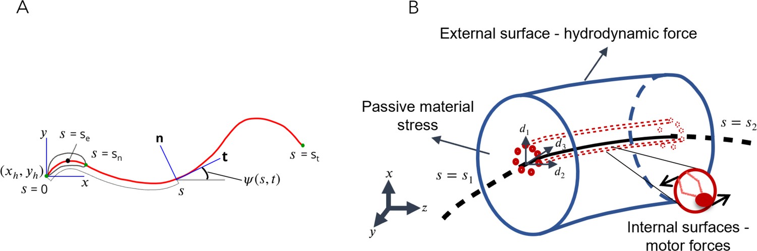
Schematic representations for the Soft, Internally driven Kirchhoff rod model.

(A) Geometric variables defined along the centerline. (B) An arbitrary control volume used for deriving the equations of the model: the volume consists of the passive flagellar material; hydrodynamic forces act on the external surface while axonemal motors act on the internal surfaces. The passive material adjacent to the cross-sectional faces at either end exerts stresses on those faces.

Figure 2

Download asset Open asset

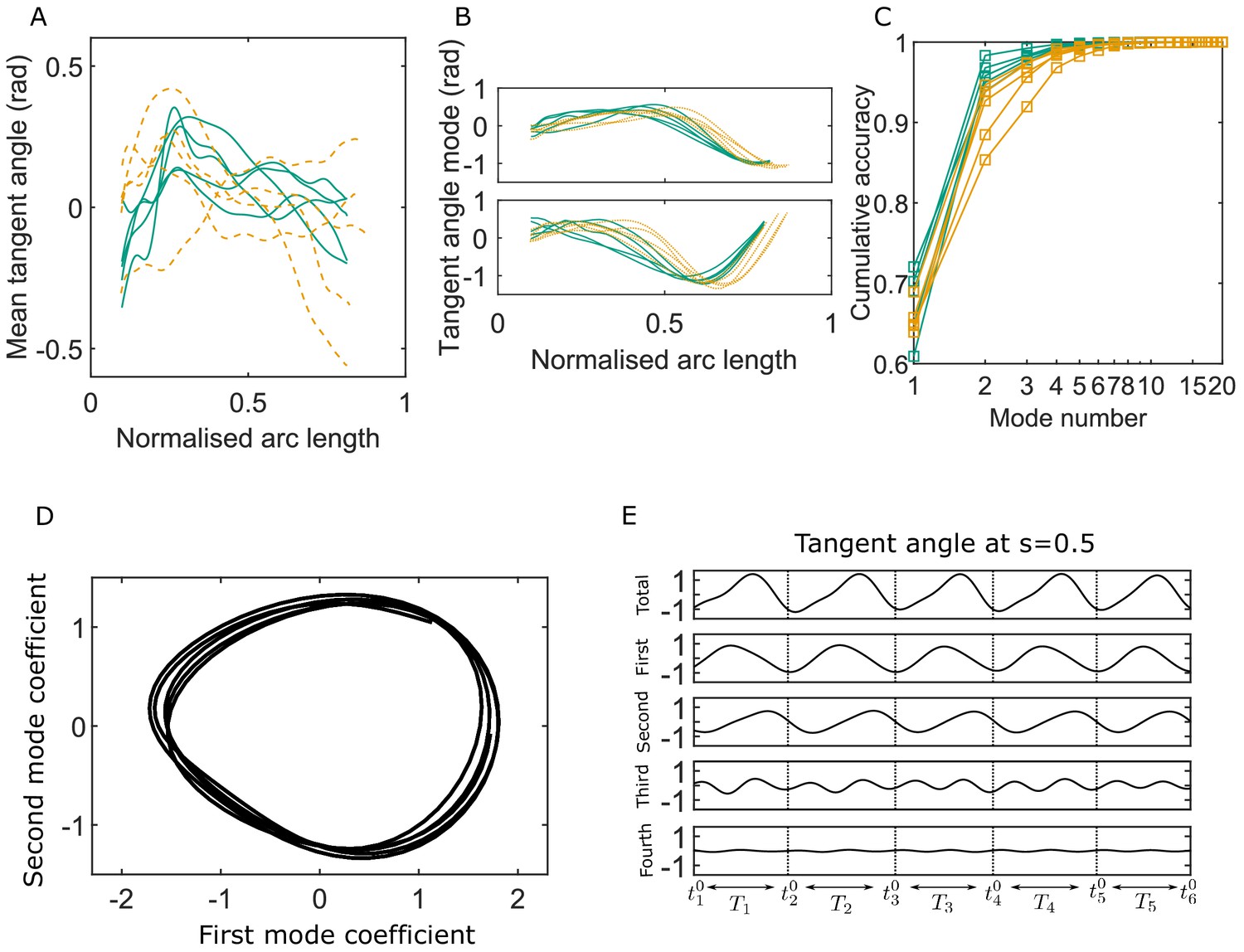
Key variables of the Chebyshev polynomial-based proper orthogonal decomposition (C-POD) of experimental tangent-angle data.

(A) Time-averaged tangent-angle profiles for five wildtype (WT) (continuous curves) and five knockout (KO) (dashed curves) samples. (B) First (top) and second (bottom) C-POD shape modes for WT (continuous curves) and KO (dashed curves) samples; the colors are as in (A). (C) Cumulative accuracy of the C-POD representation for WT and KO samples; the colors are as in (A). A representation using the first four modes captures 95% or more of the observed centerline shapes for all samples. (D) Five shape cycles for a single WT sample in the parameter space defined by the time-dependent coefficients of the first two C-POD shape modes. The zero-crossing of the second modal coefficient marks the start of a new cycle. (E) Contributions of the first four modes to the tangent angle at the midpoint of the sperm body in the five tangent-angle cycles in (D): the horizontal line in the top plot is the time-averaged tangent angle for this WT sample. The starting time of the $i$ th cycle is denoted as $t_{i}^{0}$ , and its duration (i.e., cycle time) is $T_{i}$ .

Figure 2—source data 1 Numerical data for Figure 2A, B.: https://cdn.elifesciences.org/articles/62524/elife-62524-fig2-data1-v2.mat
Download elife-62524-fig2-data1-v2.mat
Figure 2—source data 2 Numerical data for Figure 2C.: https://cdn.elifesciences.org/articles/62524/elife-62524-fig2-data2-v2.mat
Download elife-62524-fig2-data2-v2.mat
Figure 2—source data 3 Numerical data for Figure 2D.: https://cdn.elifesciences.org/articles/62524/elife-62524-fig2-data3-v2.mat
Download elife-62524-fig2-data3-v2.mat
Figure 2—source data 4 Numerical data for Figure 2E.: https://cdn.elifesciences.org/articles/62524/elife-62524-fig2-data4-v2.mat
Download elife-62524-fig2-data4-v2.mat

Figure 3

Download asset Open asset

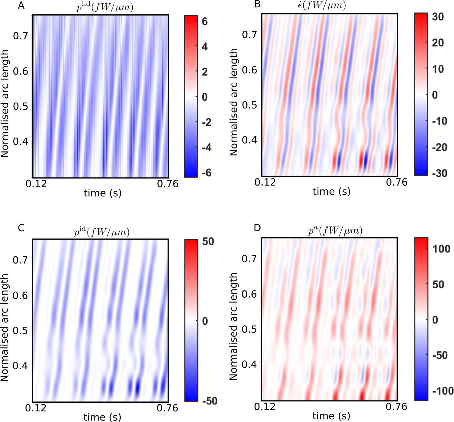
Spatiotemporal distributions of the rates of (A) hydrodynamic dissipation, (B) elastic storage, and (C) internal dissipation, and (D) the active power along the flagellum of a wildtype sperm over several beat cycles: red indicates positive rates, while blue indicates negative rates.

The data in (C) and (D) have been obtained using the scaling value of 10³ Pa s μm⁴ for the internal friction coefficient.

Figure 3—source data 1 Numerical data for all kymographs.: https://cdn.elifesciences.org/articles/62524/elife-62524-fig3-data1-v2.mat
Download elife-62524-fig3-data1-v2.mat

Figure 4

Download asset Open asset

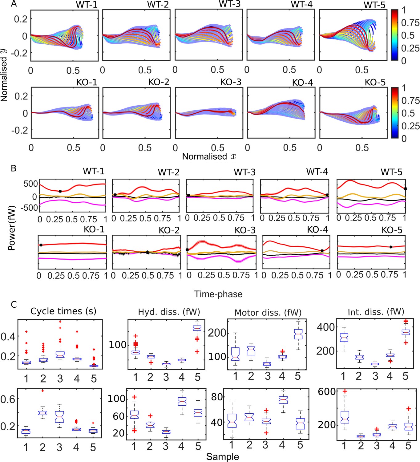
Mean cycles of beat patterns and energetics.

(A) Each colored curve shows the mean shape at a particular phase of the mean cycle for the five wildtype (WT) (top row) and knockout (KO) (bottom row) samples. The color bands around each curve indicate the standard error in the mean component. (B) Mean cycles for the magnitudes of the net elastic storage (yellow), hydrodynamic dissipation (black), internal frictional dissipation (magenta), and active power (red) in WT (top panel) and KO (bottom panel) sperm samples corresponding to those in (A). Bands show standard errors in means. (C) Statistical distributions of cycle times and dissipation rates in each of the WT (top panel) and KO (bottom panel) samples. The box-plots present the median (red line), the first and third quartile (bottom and top box edges), and minimum and maximum (lower and upper whiskers) values for 40–60 cycles. Outliers that are more than 1.5 times the interquartile range away from the top or bottom of the box are indicated by red crosses. The notch extremes correspond to $q_{2} \pm 1.57 (q_{3} - q_{1}) / \sqrt{n}$ , where q₁, q₂, and q₃ are the first, second (median), and third quartiles, respectively, and $n$ is the number of observations (McGill et al., 1978).

Figure 4—source data 1 Numerical data for Figure 4A.: https://cdn.elifesciences.org/articles/62524/elife-62524-fig4-data1-v2.mat
Download elife-62524-fig4-data1-v2.mat
Figure 4—source data 2 Numerical data for Figure 4B.: https://cdn.elifesciences.org/articles/62524/elife-62524-fig4-data2-v2.mat
Download elife-62524-fig4-data2-v2.mat
Figure 4—source data 3 Numerical data for Figure 4C (cycle times).: https://cdn.elifesciences.org/articles/62524/elife-62524-fig4-data3-v2.mat
Download elife-62524-fig4-data3-v2.mat
Figure 4—source data 4 Numerical data for Figure 4C (hyd. dissn., motor dissn., and int. dissn.).: https://cdn.elifesciences.org/articles/62524/elife-62524-fig4-data4-v2.mat
Download elife-62524-fig4-data4-v2.mat

Figure 5 with 3 supplements

Download asset Open asset

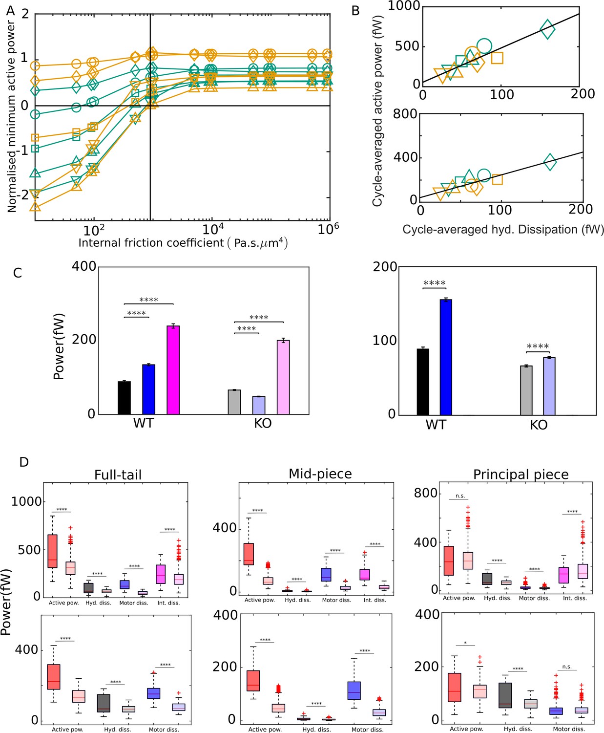
External versus internal dissipation in flagella.

(A) Effect of the value of internal friction coefficient, $η_{N}$ , on the minimum value of the net active power required to overcome dissipation for wildtype (WT) (blue) and knockout (KO) (red) samples. At each $η_{N}$ , and for each sample, the minimum in the mean cycle of the net active power, $P_{\min}$ , is normalized by the time average of the motor input, ${\bar{\bar{P}}}^{mi}$ , over all cycles. The vertical line is the scaling value of 10³ Pa s μm⁴. (B) Correlation of time averages of the hydrodynamic dissipation and net active power for $η_{N} = 10^{3}$ Pa s μm⁴(top) and 0 (bottom). The lines are linear fits through data for both species. (C) Comparison of the external hydrodynamic dissipation (black) with the motor (blue) and passive internal frictional (magenta) dissipations obtained with $η_{N} = 10^{3}$ Pa s μm⁴(left) and 0 (right). The bars represent the averages of the cycle-means of dissipations pooled from all the five sperm samples in each genotype; the error bars represent 1 standard deviation in each direction in the set of pooled cycle-means. (D) Statistical distributions of the cycle-means of powers from the WT (dark color boxes) and KO (light color boxes) samples pooled together over the entire tail (left), mid-piece (middle), and principal piece (right). The top and bottom panels are for $η_{N} = 10^{3}$ Pa s μm⁴ and 0, respectively. In (C) and (D), unpaired two-tailed t-tests are used to compare population means; **** refers to a significance level of $p \leq 10^{- 4}$ , *** $p \leq 10^{- 3}$ , ** $p \leq 10^{- 3}$ , * $p \leq 0.05$ . Differences are not significant (n.s.) when $p > 0.05$ .

Figure 5—source data 1 Numerical data for Figure 5A.: https://cdn.elifesciences.org/articles/62524/elife-62524-fig5-data1-v2.mat
Download elife-62524-fig5-data1-v2.mat
Figure 5—source data 2 Numerical data for Figure 5B.: https://cdn.elifesciences.org/articles/62524/elife-62524-fig5-data2-v2.mat
Download elife-62524-fig5-data2-v2.mat
Figure 5—source data 3 Numerical data for Figure 5C.: https://cdn.elifesciences.org/articles/62524/elife-62524-fig5-data3-v2.mat
Download elife-62524-fig5-data3-v2.mat
Figure 5—source data 4 Numerical data for Figure 5D.: https://cdn.elifesciences.org/articles/62524/elife-62524-fig5-data4-v2.mat
Download elife-62524-fig5-data4-v2.mat

Figure 5—figure supplement 1

Download asset Open asset

Comparison of population means of time-averaged dissipations obtained with the five wildtype and *Crisp2* knockout mice sperm samples obtained with (A) $η_{N}$ =10³ Pa.s.m⁴ and (B) $η_{N}$ = 0 Pa.s.m.

Error bars shown correspond to 1 standard deviation in the set of samples. Unpaired two-tailed t-tests are used to compare population means; ** $p \leq 10^{- 3}$ , * $p \leq 0.05$ . Differences are not significant (n.s.) when $p > 0.05$ .

Figure 5—figure supplement 2

Download asset Open asset

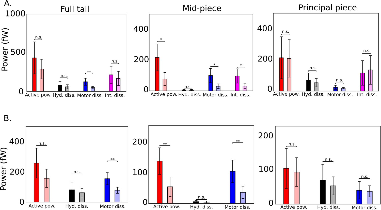
Comparison across genotypes of population means of time-averaged powers obtained with the five wildtype and *Crisp2* knockout mice sperm samples o $η_{n}$ =10³ Pa.s.m⁴ is shown in A and $η_{n}$ = 0 Pa.s.m⁴ in B.

Error bars shown correspond to 1 standard deviation in the set of samples. Unpaired two-tailed t-tests are used to compare population means; ** $p \leq 10^{- 3}$ , * $p \leq 0.05$ . Differences are not significant (n.s.) when $p > 0.05$ .

Figure 5—figure supplement 3

Download asset Open asset

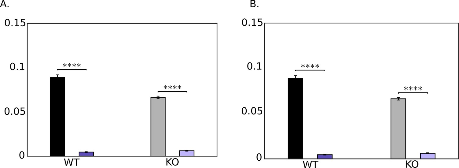
Comparison of pooled averages of the cycle-means of hydrodynamic dissipation in the tail (black) and dissipation at head due to hydrodynamic and tethering resistances (purple): $p \leq 10^{- 3}$ , * $p \leq 0.05$ . $η_{n}$ =10³ Pa.s.m⁴ is shown in A and $η_{n}$ = 0 Pa.s.m⁴ in B.

Differences are not significant (n.s.) when $p > 0.05$ .

Figure 6

Download asset Open asset

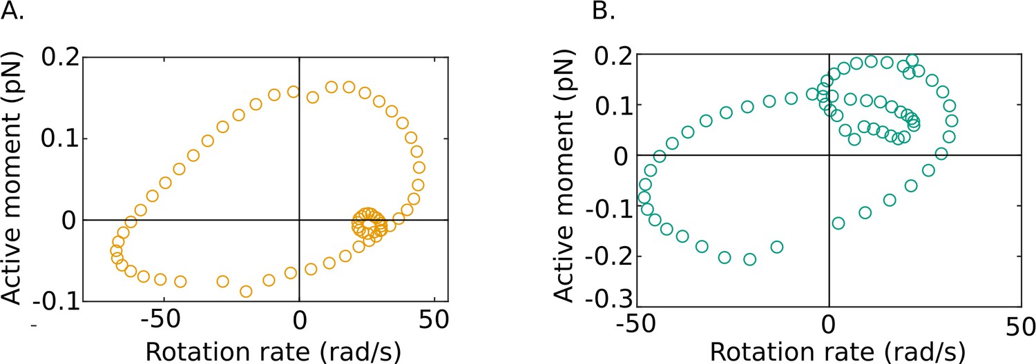
Out-of-phase mean beat cycles of active moment density and angular rotation rate at $s = 0.5$ in (A) wildtype (WT)-1 and (B) knockout (KO)-1 samples.

Figure 6—source data 1 Numerical data for Figure 6.: https://cdn.elifesciences.org/articles/62524/elife-62524-fig6-data1-v2.mat
Download elife-62524-fig6-data1-v2.mat

Figure 7

Download asset Open asset

Main steps in the image-processing algorithm shown for a single frame.

A. The original frame B. Enhanced and filtered C. Thresholded frame D. Segmented E. Skeletonized frame F. Smoothed centreline.

Appendix 2—figure 1

Download asset Open asset

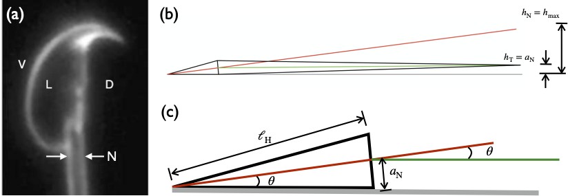
Orientation of the sperm cell with respect to the glass slide.

(a) Image from Woolley, 2003 showing the left side (L) of a mouse sperm head facing the viewer with the ventral (V) and dorsal (D) sides of the head indicated. The concave side of the hook is towards the dorsal side. Also shown is the neck (N) at the proximal end of the flagellum. (b) Schematic showing the mouse sperm body as viewed from its dorsal side when the left side of its head is against the wall. The intrinsic angle made by the head with the flagellum at the neck enables planar beating when the left side of the head is against the wall. The red and green lines indicate the axes of the head and the tail. In this orientation, the flagellum beats in a plane parallel to the wall and its centerline is at a distance equal to the neck radius , $a_{n}$ , from the wall. If there had been no angle at the neck, the tip of the tail would be at a height of $h_{t} = h_{\max}$ . (c) The angle (in radians) of the head axis to the wall, $θ \approx a_{n} / ℓ_{h}$ .

Author response image 1

Download asset Open asset

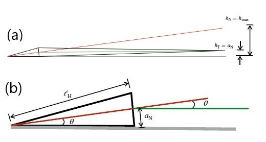
(a) Schematic showing the mouse sperm body as viewed from its dorsal side when the left side of its head is against the wall. The intrinsic angle made by the head with the flagellum at the neck enables planar beating when the left side of the head is against the wall. The red and green lines indicate the axes of the head and the tail. In this orientation, the flagellum beats in a plane parallel to the wall and its centreline is at a distance equal to the neck radius ,an, from the wall. If there had been no angle at the neck, the tip of the tail would be at a height of h_T = h_max. (b) The angle (in radians) of the head axis to the wall, θ ≈ an/ ℓh.

Author response image 2

Download asset Open asset

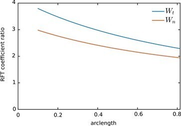
Ratio of the Wall-RFT coefficients in revised manuscript to the bulk coefficients in the original submission.

Author response image 3

Download asset Open asset

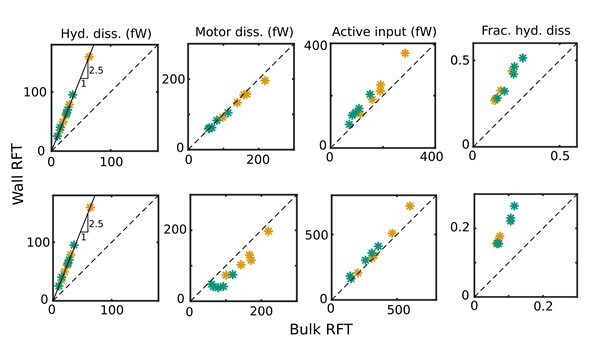
Comparison of revised values of the cycle-means of (i) hydrodynamic dissipation, (ii) motor dissipation, (iii) active power input, and (iv) the proportion of hydrodynamic dissipation out of the total dissipation against their values in the original manuscript for WT (green symbols) and KO (yellow symbols) samples, with ηn = 0 (top panel) and 103 Pa s µm⁴(bottom panel): the values in the original submission are along the horizontal axes and the revised values are along the vertical axes.

Tables

Key resources table

Reagent type (species) or resource	Designation	Source or reference	Identifiers	Additional information
Gene (Mus musculus)	Crisp2	Lim et al., 2019	-	-
Strain, strain background (Mus musculus)	C57BL/6N	Lim et al., 2019	PMID:30759213	Mice produced through the Australian Phenomics Network
Biological sample (Mus musculus)	Sperm	Lim et al., 2019	-	Collected from the cauda epididymis and vas deferens using the backflushing method
Chemical compound, drug	TYH medium with 0.3 mg/ml BSA	Lim et al., 2019	-	Buffer media for sperm
Software, algorithm	MATLAB, MATLAB Image Processing Toolbox, Fiji		SCR 001622,SCR 002285	Code (Nandagiri, 2021) and original videos (Nandagiri et al., 2020) available for public access

Appendix 3—table 1

One-way ANOVA data for establishing that sample means of cycle variables are significantly different from population means in the wildtype (WT) and knockout (KO) genotypes; $F$ denotes the $F$ -test statistic and $p$ denotes probability of the null hypothesis.

Genotype	Flagellar region	Power	Treatments DOF	Error DOF	$F$	$p$
WT	Full	Cycle time	4	306	50.31	$< 10^{- 16}$
WT	Full	Input power	4	306	833.19	$< 10^{- 16}$
WT	Full	Hyd. dissn.	4	306	1441.37	$< 10^{- 16}$
WT	Full	Internal dissn.	4	306	730.68	$< 10^{- 16}$
WT	Full tail	Motor dissn.	4	306	246.17	$< 10^{- 16}$
WT	Mid-piece	Input power	4	306	483.02	$< 10^{- 16}$
WT	Mid-piece	Hyd. dissn.	4	306	186.86	$< 10^{- 16}$
WT	Mid-piece	Internal dissn.	4	306	436.92	$< 10^{- 16}$
WT	Mid-piece	Motor dissn.	4	306	421.04	$< 10^{- 16}$
WT	Principal piece	Input power	4	306	786.93	$< 10^{- 16}$
WT	Principal piece	Hyd. disspn.	4	306	1716.31	$< 10^{- 16}$
WT	Principal piece	Internal dissn.	4	306	520.19	$< 10^{- 16}$
WT	Principal piece	Motor dissn.	4	306	140.96	$< 10^{- 16}$
KO	Full tail	Cycle time	4	270	235.45	$< 10^{- 16}$
KO	Full tail	Input power	4	270	110.04	$< 10^{- 16}$
KO	Full tail	Hyd. dissn.	4	270	198.37	$< 10^{- 16}$
KO	Full tail	Internal dissn.	4	270	90.02	$< 10^{- 16}$
KO	Full tail	Motor dissn.	4	270	120.31	$< 10^{- 16}$
KO	Mid-piece	Input power	4	270	528.12	$< 10^{- 16}$
KO	Mid-piece	Hyd. dissn.	4	270	216.51	$< 10^{- 16}$
KO	Mid-piece	Internal dissn.	4	270	247.53	$< 10^{- 16}$
KO	Mid-piece	Motor dissn.	4	270	374.02	$< 10^{- 16}$
KO	Principal piece	Input power	4	270	125.73	$< 10^{- 16}$
KO	Principal piece	Hyd. dissn.	4	270	206.07	$< 10^{- 16}$
KO	Principal piece	Internal dissn.	4	270	109.09	$< 10^{- 16}$
KO	Principal piece	Motor dissn.	4	270	20.3	$< 10^{- 16}$

Appendix 3—table 2

Comparison of the external hydrodynamic dissipation with the internal frictional and motor dissipations: $t$ denotes the Student's $t$ -test statistic in an unpaired, two-tailed test; $p$ is the probability of the null hypothesis.

Genotype	Flagellar region	$η_{n}$ (Pa s μm⁴)	Hyd. dissn. (fW)	Int. dissn. (fW)	$t$	$p$
WT	Full tail	10³	89.07	240.05	22.71	$< 10^{- 16}$
WT	Mid-piece	10³	6.69	108.43	36.39	$< 10^{- 16}$
WT	Principal piece	10³	82.21	131.11	9.82	$< 10^{- 16}$
KO	Full tail	10³	66.39	200.91	21.44	$< 10^{- 16}$
KO	Mid-piece	10³	4.80	32.40	29.16	$< 10^{- 16}$
KO	Principal piece	10³	61.48	168.28	16.73	$< 10^{- 16}$
Genotype	Flagellar region	$η_{n}$ (Pa s μm⁴)	Hyd. dissn. (fW)	Motor dissn. (fW)	$t$	$p$
WT	Full tail	10³	89.07	135.06	11.48	$< 10^{- 16}$
WT	Mid-piece	10³	6.69	109.75	36.21	$< 10^{- 16}$
WT	Principal piece	10³	82.21	25.09	20.71	$< 10^{- 16}$
KO	Full tail	10³	66.39	48.72	9.74	$< 10^{- 16}$
KO	Mid-piece	10³	4.80	29.14	24.87	$< 10^{- 16}$
KO	Principal piece	10³	61.48	19.49	28.4	$< 10^{- 16}$
WT	Full tail	0	89.07	155.58	11.48	$< 10^{- 16}$
WT	Mid-piece	0	6.69	112.56	36.21	$< 10^{- 16}$
WT	Principal piece	0	82.21	42.71	20.71	$< 10^{- 16}$
KO	Full tail	0	66.39	77.61	9.74	$< 10^{- 16}$
KO	Full tail	0	4.80	35.23	24.87	$< 10^{- 16}$
KO	Principal piece	0	61.48	42.28	28.4	$< 10^{- 16}$

Appendix 3—table 3

Comparison of wildtype (WT) and knockout (KO) samples.

The values in in columns 2 and 3 are the means of the distributions created by pooling together values from the individual cycles of all the sperm samples in each genotype.

Quantity	WT	KO	$t$	$p$
Cycle time (s)	0.16	0.18	2.72	0.01
Reciprocal cycle time (Hz)	7.19	7.2	0.03501	0.97
Full tail hyd. dissn. (fW)	89.07	66.39	6.91	1.26 × 10⁻¹¹
Mid-piece hyd. dissn. (fW)	6.69	4.80	6.89	1.49 × 10⁻¹¹
Principal piece hyd. dissn. (fW)	82.21	61.48	6.71	4.63 × 10⁻¹¹
Full tail motor dissn. (fW), $η_{n} = 10^{3}$ Pa s μm⁴	135.06	48.72	26.89	$< 10^{- 16}$
Full tail int. dissn. (fW), $η_{n} = 10^{3}$ Pa s μm⁴	240.05	200.91	4.55	6.54 × 10⁻⁶
Mid-piece motor disspn. (fW), $η_{n} = 10^{3}$ Pa s μm⁴	109.75	29.14	25.57	$< 10^{- 16}$
Mid-piece int. dissn. (fW), $η_{n} = 10^{3}$ Pa s μm⁴	108.43	32.40	24.59	$< 10^{- 16}$
Principal piece motor dissn. (fW), $η_{n} = 10^{3}$ Pa s μm⁴	25.08	19.49	5.62	3.01 × 10⁻⁸
Principal piece int. dissn. (fW), $η_{n} = 10^{3}$ Pa s μm⁴	131.11	168.28	5.03	3.01 × 10⁻⁸
Full tail motor dissn. (fW), $η_{n} = 0$ Pa s μm⁴	155.58	77.61	24.87	$< 10^{- 16}$
Mid-piece motor dissn. (fW), $η_{n} = 0$ Pa s μm⁴	112.56	35.23	29.10	$< 10^{- 16}$
Principal piece motor dissn. (fW), $η_{n} = 0$ Pa s μm⁴	42.71	42.28	0.22	0.82

Additional files

Transparent reporting form: https://cdn.elifesciences.org/articles/62524/elife-62524-transrepform-v2.docx
Download elife-62524-transrepform-v2.docx

Download links

A two-part list of links to download the article, or parts of the article, in various formats.

Downloads (link to download the article as PDF)

Open citations (links to open the citations from this article in various online reference manager services)

Mendeley

Cite this article (links to download the citations from this article in formats compatible with various reference manager tools)

Ashwin Nandagiri
Avinash Satish Gaikwad
David L Potter
Reza Nosrati
Julio Soria
Moira K O'Bryan
Sameer Jadhav
Ranganathan Prabhakar

(2021)

Flagellar energetics from high-resolution imaging of beating patterns in tethered mouse sperm

eLife 10:e62524.

https://doi.org/10.7554/eLife.62524

Figures

Schematic representations for the Soft, Internally driven Kirchhoff rod model.

Key variables of the Chebyshev polynomial-based proper orthogonal decomposition (C-POD) of experimental tangent-angle data.

Figure 2—source data 1

Figure 2—source data 2

Figure 2—source data 3

Figure 2—source data 4

Spatiotemporal distributions of the rates of (A) hydrodynamic dissipation, (B) elastic storage, and (C) internal dissipation, and (D) the active power along the flagellum of a wildtype sperm over several beat cycles: red indicates positive rates, while blue indicates negative rates.

Figure 3—source data 1

Mean cycles of beat patterns and energetics.

Figure 4—source data 1

Figure 4—source data 2

Figure 4—source data 3

Figure 4—source data 4

External versus internal dissipation in flagella.

Figure 5—source data 1

Figure 5—source data 2

Figure 5—source data 3

Figure 5—source data 4

Comparison of population means of time-averaged dissipations obtained with the five wildtype and Crisp2 knockout mice sperm samples obtained with (A) $η_{N}$ =10³ Pa.s.m⁴ and (B) $η_{N}$ = 0 Pa.s.m.

Comparison across genotypes of population means of time-averaged powers obtained with the five wildtype and Crisp2 knockout mice sperm samples o $η_{n}$ =10³ Pa.s.m⁴ is shown in A and $η_{n}$ = 0 Pa.s.m⁴ in B.

Comparison of pooled averages of the cycle-means of hydrodynamic dissipation in the tail (black) and dissipation at head due to hydrodynamic and tethering resistances (purple): $p \leq 10^{- 3}$ , * $p \leq 0.05$ . $η_{n}$ =10³ Pa.s.m⁴ is shown in A and $η_{n}$ = 0 Pa.s.m⁴ in B.

Out-of-phase mean beat cycles of active moment density and angular rotation rate at $s = 0.5$ in (A) wildtype (WT)-1 and (B) knockout (KO)-1 samples.

Figure 6—source data 1

Main steps in the image-processing algorithm shown for a single frame.

Orientation of the sperm cell with respect to the glass slide.

Ratio of the Wall-RFT coefficients in revised manuscript to the bulk coefficients in the original submission.

Tables

One-way ANOVA data for establishing that sample means of cycle variables are significantly different from population means in the wildtype (WT) and knockout (KO) genotypes; $F$ denotes the $F$ -test statistic and $p$ denotes probability of the null hypothesis.

Comparison of the external hydrodynamic dissipation with the internal frictional and motor dissipations: $t$ denotes the Student's $t$ -test statistic in an unpaired, two-tailed test; $p$ is the probability of the null hypothesis.

Comparison of wildtype (WT) and knockout (KO) samples.

Additional files

Transparent reporting form

Download links

Downloads (link to download the article as PDF)

Open citations (links to open the citations from this article in various online reference manager services)

Cite this article (links to download the citations from this article in formats compatible with various reference manager tools)

Be the first to read new articles from eLife

Share this article

Cite this article

Schematic representations for the Soft, Internally driven Kirchhoff rod model.

Key variables of the Chebyshev polynomial-based proper orthogonal decomposition (C-POD) of experimental tangent-angle data.

Figure 2—source data 1

Figure 2—source data 2

Figure 2—source data 3

Figure 2—source data 4

Spatiotemporal distributions of the rates of (A) hydrodynamic dissipation, (B) elastic storage, and (C) internal dissipation, and (D) the active power along the flagellum of a wildtype sperm over several beat cycles: red indicates positive rates, while blue indicates negative rates.

Figure 3—source data 1

Mean cycles of beat patterns and energetics.

Figure 4—source data 1

Figure 4—source data 2

Figure 4—source data 3

Figure 4—source data 4

External versus internal dissipation in flagella.

Figure 5—source data 1

Figure 5—source data 2

Figure 5—source data 3

Figure 5—source data 4

Comparison of population means of time-averaged dissipations obtained with the five wildtype and Crisp2 knockout mice sperm samples obtained with (A) ηN=103 Pa.s.m4 and (B) ηN = 0 Pa.s.m.

Comparison across genotypes of population means of time-averaged powers obtained with the five wildtype and Crisp2 knockout mice sperm samples o ηn=103 Pa.s.m4 is shown in A and ηn = 0 Pa.s.m4 in B.

Comparison of pooled averages of the cycle-means of hydrodynamic dissipation in the tail (black) and dissipation at head due to hydrodynamic and tethering resistances (purple): p≤10-3, *p≤0.05. ηn=103 Pa.s.m4 is shown in A and ηn = 0 Pa.s.m4 in B.

Out-of-phase mean beat cycles of active moment density and angular rotation rate at s=0.5 in (A) wildtype (WT)-1 and (B) knockout (KO)-1 samples.

Figure 6—source data 1

Main steps in the image-processing algorithm shown for a single frame.

Orientation of the sperm cell with respect to the glass slide.

Ratio of the Wall-RFT coefficients in revised manuscript to the bulk coefficients in the original submission.

One-way ANOVA data for establishing that sample means of cycle variables are significantly different from population means in the wildtype (WT) and knockout (KO) genotypes; F denotes the F-test statistic and p denotes probability of the null hypothesis.

Comparison of the external hydrodynamic dissipation with the internal frictional and motor dissipations: t denotes the Student's t-test statistic in an unpaired, two-tailed test; p is the probability of the null hypothesis.

Comparison of wildtype (WT) and knockout (KO) samples.

Transparent reporting form

Downloads (link to download the article as PDF)

Open citations (links to open the citations from this article in various online reference manager services)

Cite this article (links to download the citations from this article in formats compatible with various reference manager tools)

Comparison of population means of time-averaged dissipations obtained with the five wildtype and Crisp2 knockout mice sperm samples obtained with (A) $η_{N}$ =10³ Pa.s.m⁴ and (B) $η_{N}$ = 0 Pa.s.m.

Comparison across genotypes of population means of time-averaged powers obtained with the five wildtype and Crisp2 knockout mice sperm samples o $η_{n}$ =10³ Pa.s.m⁴ is shown in A and $η_{n}$ = 0 Pa.s.m⁴ in B.

Comparison of pooled averages of the cycle-means of hydrodynamic dissipation in the tail (black) and dissipation at head due to hydrodynamic and tethering resistances (purple): $p \leq 10^{- 3}$ , * $p \leq 0.05$ . $η_{n}$ =10³ Pa.s.m⁴ is shown in A and $η_{n}$ = 0 Pa.s.m⁴ in B.

Out-of-phase mean beat cycles of active moment density and angular rotation rate at $s = 0.5$ in (A) wildtype (WT)-1 and (B) knockout (KO)-1 samples.

One-way ANOVA data for establishing that sample means of cycle variables are significantly different from population means in the wildtype (WT) and knockout (KO) genotypes; $F$ denotes the $F$ -test statistic and $p$ denotes probability of the null hypothesis.

Comparison of the external hydrodynamic dissipation with the internal frictional and motor dissipations: $t$ denotes the Student's $t$ -test statistic in an unpaired, two-tailed test; $p$ is the probability of the null hypothesis.