Figures and data in Bayesian inference of kinetic schemes for ion channels by Kalman filtering

Version of Record

Accepted for publication after peer review and revision.

Download
Cite
Share
CommentOpen annotations (there are currently 0 annotations on this page).

Version of Record updated: February 9, 2024 (This version)
Version of Record published: August 1, 2022 (Go to version)
Accepted Manuscript published: May 4, 2022 (Go to version)
Accepted: April 22, 2022
Received: September 2, 2020
Preprint posted: April 28, 2020 (Go to version)

Figures
Tables
Additional files

27 figures, 3 tables and 2 additional files

Figures

Box 1—figure 1

Download asset Open asset

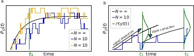
The First-order Markov property of the data requires a recursive prediction of the signal (by the model) and correction (by the data) scheme of the algorithm.

(a) Idealized patch-clamp (PC) data in the absence of instrumental noise for either ten (colored) or an infinite number of channels generating the mean time trace (black). The fluctuations with respect to the mean time trace (black) reveal autocorrelation (b) Conceptual idea of the Kalman Filter (KF): the stochastic evolution of the ensemble signal is predicted and the prediction model updated recursively.

Box 1—figure 2

Download asset Open asset

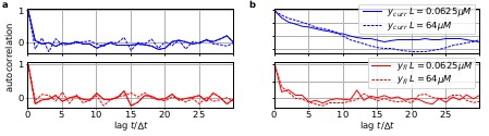
The residuals between model prediction and data reveal long autocorrelations if the analysis algorithm ignores the first-order Markov property.

(a) Autocorrelation of the residuals $r_{I}$ of two ligand concentrations of currents (blue) and of the fluorescence (red) after the data have been analyzed with the KF approach. (b) autocorrelation of $r_{I}$ after analysing with he RE approach.

Figure 1

Download asset Open asset

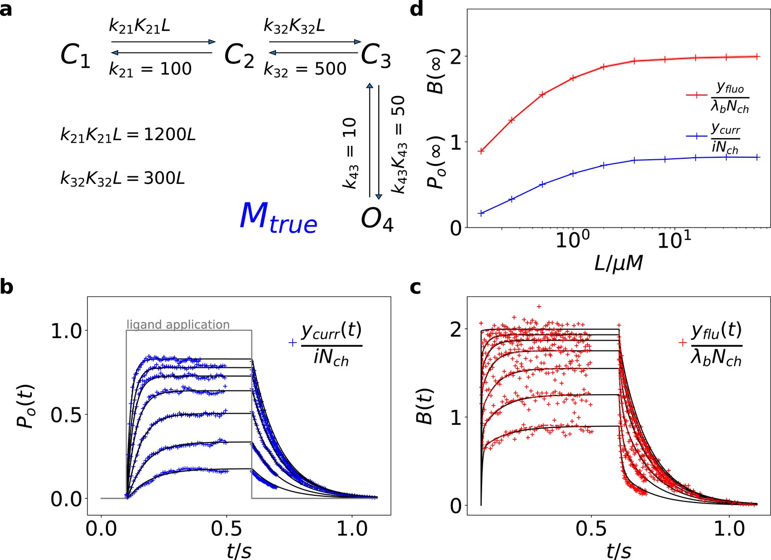
Kinetic scheme and simulated data.

(a) The Markov state model (kinetic scheme) consists of two binding steps and one opening step. The rate matrix $K$ is parametrized by the absolute rates $k_{i j}$ , the ratios $K_{i j}$ between on and off rates (i.e. equilibrium constants) and $L$ , the ligand concentration in the solution. The units of the rates are $s^{- 1}$ and $μ M^{- 1} s^{- 1}$ , respectively. The liganded states are C₂, C₃, O₄. The open state O₄ conducts a mean single-channel current $i = 1$ . Note, that absolute magnitude of the single channel current is irrelevant regarding this study what matters is its relative magnitude compared with $σ_{op}$ and $σ_{ex}$ . Simulations were performed with 10 kHz or 100 kHz (for Figures 11 and 12) sampling, KF analysis frequency f_ana for cPCF data is in the range of (200-500) Hz while pure current data is analyzed at 2-5 kHz. (**b-c**) Normalized time traces of simulated relaxation experiments of ligand concentration jumps with $N_{ch} = 10^{3}$ channels, $λ_{b} = 0.375$ mean photons per bound ligand per frame and single-channel current $i = 1$ , open-channel noise with $σ_{op}^{2} = 0.1 i^{2}$ and an instrumental noise with the variance $σ_{m}^{2} = i^{2}$ . The current y_curr and fluorescence y_flu time courses are calculated from the same simulation. For visualization, the signals are normalized by the respective median estimates of the KF. The black lines are the theoretical open probabilities $P_{o} (t)$ and the average binding per channel $B (t)$ for $N_{ch} \to \infty$ of the used model. Typically, we used 10 ligand concentrations which are (0.0625, 0.125, 0.25, 0.5, 1, 2,4, 8, 16, 64) $μ M$ . d, Equilibrium binding and open probability as function of the ligand concentration $L$ .

Figure 1—source data 1 The example data is provided.: https://cdn.elifesciences.org/articles/62714/elife-62714-fig1-data1-v3.zip
Download elife-62714-fig1-data1-v3.zip

Figure 2

Download asset Open asset

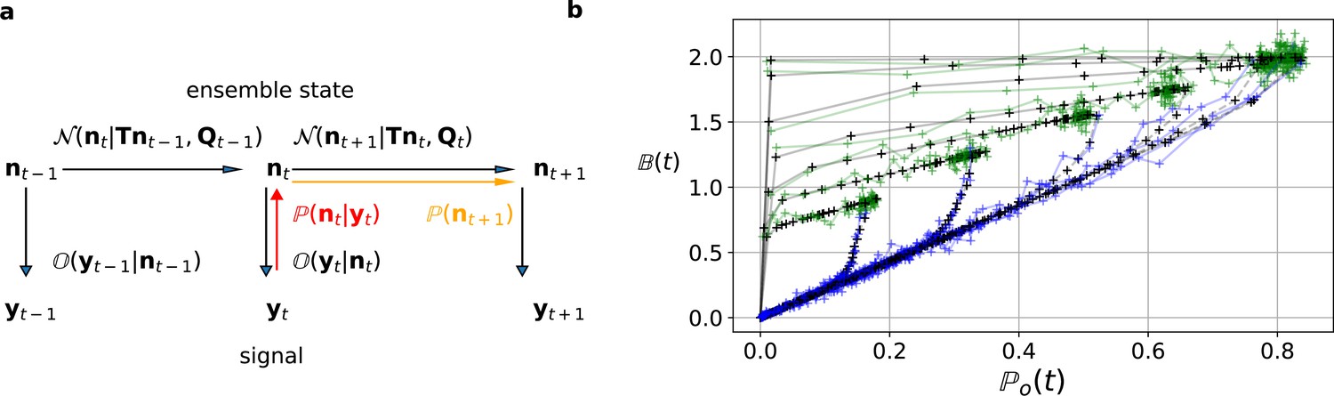
The first-order hidden Markov structure is explicitly used by the Bayesian filter.

The filter can be seen as continuous state analog of the forward algorithm. (a) Graphical model of the conditional dependencies of the stochastic process. Horizontal black arrows represent the conditional multivariate normal transition probability $N (n_{t + 1} | T n_{t}, Q_{t})$ of a continuous state Markov process. Notably, it is $n (t)$ which is treated as the Markov state by the KF. The transition matrix $T$ and the time-dependent covariance $Q_{t} = Q (T, n_{t})$ characterise the single-channel dynamics. The vertical black arrows represent the conditional observation distribution $O (y_{t} | n_{t})$ . The observation distribution summarizes the noise of the experiment, which in the KF is assumed to be multivariate normal. Given a set of model parameters and a data point $y_{t}$ , the Bayesian theorem allows to calculate in the correction step $P (n_{t} | y_{t})$ (red arrow). The posterior is propagated linearly in time by the model, predicting a state distribution $P (n_{t + 1})$ (orange arrow). The propagated posterior predicts together with the observation distribution the mean and covariance of the next observation. Thus, it creates a multivariate normal likelihood for each data point in the observation space. (b) Observation space trajectories of the predictions and data of the binding per channel vs. open probability for different ligand concentrations. The curves are normalized by the median estimates of $λ_{b}$ , $i$ and $N_{c h}$ and the ratio of open-channels $\frac{y_{c u r r}}{N_{c h} i}$ which approximates the open probability $P_{o} (t)$ . The black crosses represent the predicted mean signal $H E [n_{t + 1}]$ , which is calculated by multiplying the observational matrix $H$ with the mean predicted state $E [n_{t + 1}]$ . For clarity, we used the mean value of the posterior of the KF. The green and blue trajectories represent the part of the time traces with after the jump to non-zero ligand concentration and after jumping backt to zero ligand concentration in the bulk, respectively.

Figure 3

Download asset Open asset

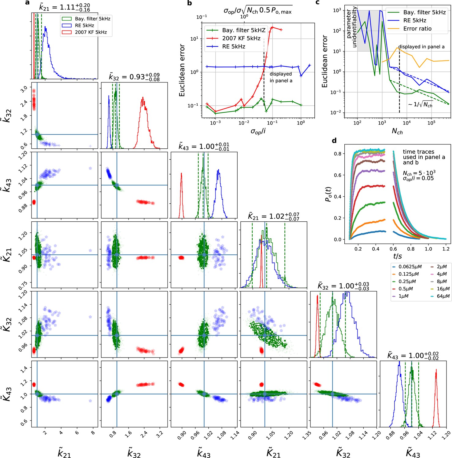
The Bayesian filter overcomes the sensitivity to varying (open-channel) noise of the classic Kalman filter and does not show the overconfidence of the RE-approach.

Overall it shows the highest accuracy and the posterior covers the true values. The classical deterministic RE (blue), 2007 Kalman filter (red) and our Bayesian filter (green) are implemented as a full Bayesian version and the obtained posterior distributions are compared. For all PC data sets in the figure the analysing frequencies $f_{ana}$ ranges within 2-5. (a) Posterior of the parameters for the 3 algorithms for the data set displayed in panel d. The blue crosses indicate the true values. All samples are normalized by their true values which is indicated by the ∼ above the parameters. For clarity, we only show a fraction of the samples of the posterior for blue and red. b, Effect of open channel noise: The Euclidean error for all three approaches is plotted vs. $σ_{op} / i$ (low axis).The upper axis displays the ratio of the ‘typical’ standard deviation of the open channel excess noise of the ensemble of channels $σ_{o p} \sqrt{N 0.5 P_{o, m a x}}$ to the standard deviation of instrumental noise. c, Influence of patch size: Scaling of the Euclidean error vs. $N_{c h}$ follows $\sim (N_{c h})^{- 0.5}$ indicated by the dashed lines for $N_{ch} > 2 \cdot 10^{3}$ for the RE and the Bayesian filter approach. The data indicates a constant error ratio (orange) for large $N_{ch}$ . For $N_{c h} < 2 \cdot 10^{3}$ samples of the posteriors for many data sets suggest an improper posterior. An instrumental noise of $σ_{e x} / i = 1$ and $σ_{o p} / i = 0.01$ was used. (d) The time traces on which the posteriors of panel a are based (for the ligand concentrations see Figure 1). Panel b used the same data too, but σ and $σ_{o p}$ were varied.

Figure 3—source data 1 The data folder includes all 15 sets of time traces.: https://cdn.elifesciences.org/articles/62714/elife-62714-fig3-data1-v3.zip
Download elife-62714-fig3-data1-v3.zip

Figure 4

Download asset Open asset

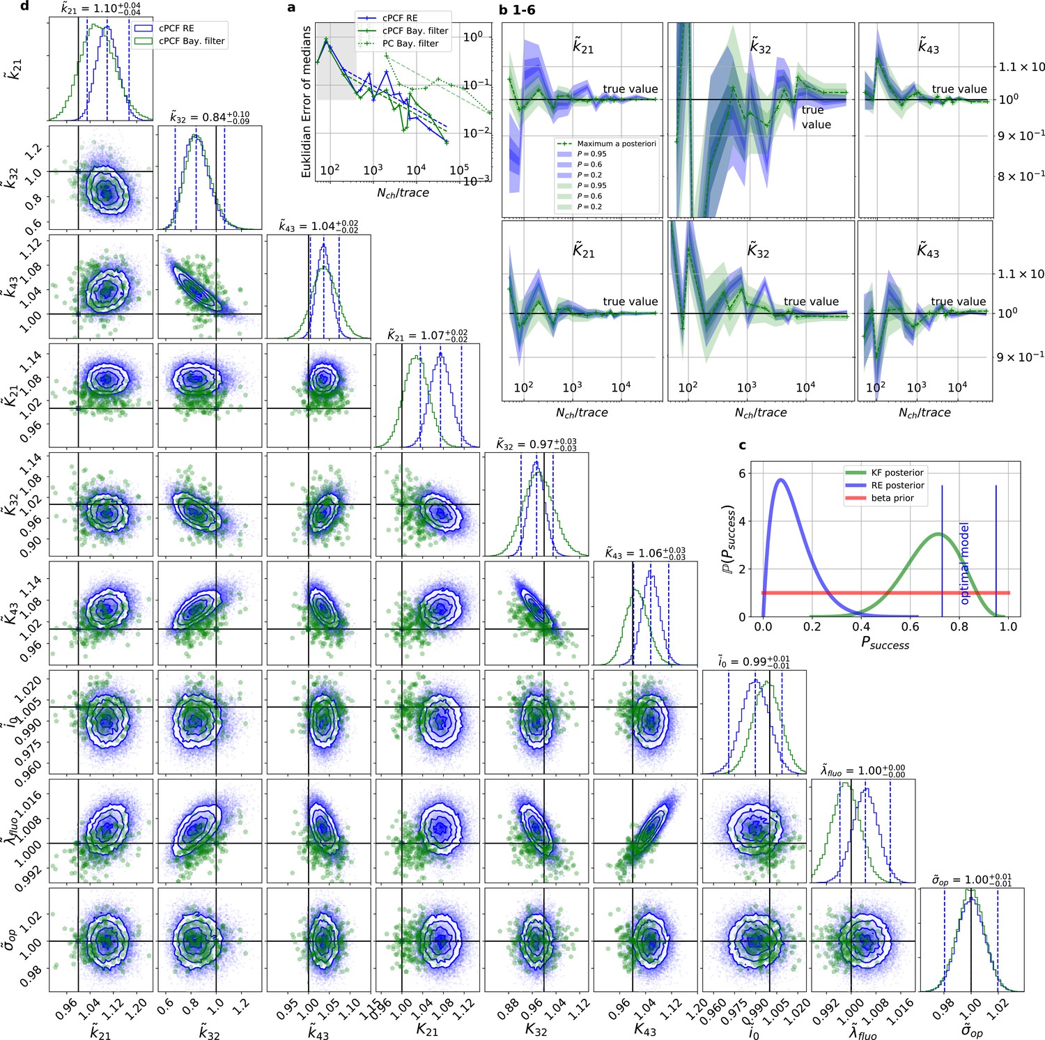
For multidimensional data (cPCF) the RE approach almost approaches the accuracy (Euclidean error) of the Bayesian Filter.

However, only the Bayesian filter covers the true value in a reasonable HDCV while RE based posteriors are too narrow. All samples are normalized by their true values which is indicated by the ∼ above the parameters. (a) Euclidean errors of the maximum for the rate $k_{i j}$ and equilibrium constants $K_{i j}$ obtained by the KF (green) and from the REs (blue) are plotted against $N_{c h}$ for $σ_{e x} / i = 0.5$ , $σ_{o p} / i = 0.05$ and $λ_{b} = 5$ . Both algorithms scale like $1 / \sqrt{N_{c h}}$ (dashed lines) for larger $N_{c h}$ which is the expected scaling For smaller $N_{c h} < 500$ (gray range) the error is roughly the same indicating that limitations of the normal approximation to the multinomial distribution dominate the overall error in this regime. The combination of fluorescence and current data(cPCF) decreases the eucleadian error for both approaches compared to current data alone(PC). (b), HDCI and the mode of the 3 $k_{i j}$ and 3 $K_{i j}$ plotted vs. $N_{c h}$ revealing that the maximum is a consistent estimator (converges in distribution to the true value with increasing data quality). While the KF (green) 0.95-HDCI includes usually the true value, the RE HDCI (blue) is too narrow and, thus, the real values are frequently not included. (c) Bayesian estimation of true success probability for the event that all 6 0.95-HDCI include the respective true values at the same time by a binomial likelihood. Since the data sets have different $N_{c h}$ and the model approximations become better with increasing $N_{ch}$ , we use a cut-off for $N_{c h} = 200$ . d, Comparison of 1-D and combinations of 2-D marginal posteriors of the parameters of interest for both algorithms calculated from a $N_{c h} = 10^{3}$ simulation. Blue lines indicate the true value. We depict that in two dimensions the disproportion of the deviation of the mode and the spread of RE (blue) approach is worsened while KF (green) posterior includes the true values with more reasonable probability mass.

Figure 4—source data 1 6µMol. Each of the source data folders contains for a specific ligand concentration the time traces of cPCF data for all $N_{ch}$ .: https://cdn.elifesciences.org/articles/62714/elife-62714-fig4-data1-v3.zip
Download elife-62714-fig4-data1-v3.zip
Figure 4—source data 2 64µMol.: https://cdn.elifesciences.org/articles/62714/elife-62714-fig4-data2-v3.zip
Download elife-62714-fig4-data2-v3.zip
Figure 4—source data 3 32µMol.: https://cdn.elifesciences.org/articles/62714/elife-62714-fig4-data3-v3.zip
Download elife-62714-fig4-data3-v3.zip
Figure 4—source data 4 8µMol.: https://cdn.elifesciences.org/articles/62714/elife-62714-fig4-data4-v3.zip
Download elife-62714-fig4-data4-v3.zip
Figure 4—source data 5 4µMol.: https://cdn.elifesciences.org/articles/62714/elife-62714-fig4-data5-v3.zip
Download elife-62714-fig4-data5-v3.zip
Figure 4—source data 6 1µMol.: https://cdn.elifesciences.org/articles/62714/elife-62714-fig4-data6-v3.zip
Download elife-62714-fig4-data6-v3.zip
Figure 4—source data 7 2µMol.: https://cdn.elifesciences.org/articles/62714/elife-62714-fig4-data7-v3.zip
Download elife-62714-fig4-data7-v3.zip
Figure 4—source data 8 025µMol.: https://cdn.elifesciences.org/articles/62714/elife-62714-fig4-data8-v3.zip
Download elife-62714-fig4-data8-v3.zip
Figure 4—source data 9 05µMol.: https://cdn.elifesciences.org/articles/62714/elife-62714-fig4-data9-v3.zip
Download elife-62714-fig4-data9-v3.zip
Figure 4—source data 10 00625µMol.: https://cdn.elifesciences.org/articles/62714/elife-62714-fig4-data10-v3.zip
Download elife-62714-fig4-data10-v3.zip
Figure 4—source data 11 003125µMol.: https://cdn.elifesciences.org/articles/62714/elife-62714-fig4-data11-v3.zip
Download elife-62714-fig4-data11-v3.zip
Figure 4—source data 12 0125µMol.: https://cdn.elifesciences.org/articles/62714/elife-62714-fig4-data12-v3.zip
Download elife-62714-fig4-data12-v3.zip

Figure 5

Download asset Open asset

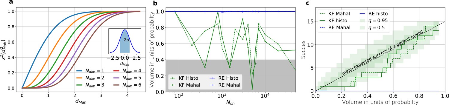
The HDCV of the posterior of the KF follows the requested binomial statistics while the HDCVs of the RE approach are too narrow.

(a) Cumulative χ-square distribution vs. the Mahalanobis distance $d_{Mah}$ . The y axis denotes the probability mass which is counted by moving away from the maximum before an ellipsoid with distance $d_{Mah}$ is reached. The different colours represent the changes of the cdf with an increasing number of rate parameters. The blue cdf at $d_{Mah} = 1$ represents how much probability mass can be found from $\int_{- σ}^{σ} normal (θ, 0, σ) d θ$ , see inset. In one dimension, we can expect to find the true value within $2 σ$ around the mean with the usual probability of $P = 0.682$ for univariate normally distributed random variables. The six parameters (brown) of the full rate matrix will almost certainly be beyond $d_{Mah} = 1.0$ . The higher the dimensions of the space the less important becomes the maximum of the probability density distribution for the typical set which is by definition the region where the probability mass resides. The mathematical reason for this is that the probability mass $P = \int_{V} ℙ (θ) d V$ is the integrated product of volume and probability density. b, The two methods to count volume in units of probability mass for the KF (green) and the RE (blue). The gray area indicates which data sets are considered a success if one chooses to evaluate a proababilty mass of 0.4 of each posterior around its mode. All data sets in the white area are considered a failure. For the optimistic noise assumptions $σ_{ex} = 0.5 \cdot i$ , $σ_{op} = 0.05 \cdot i$ and a mean photon count per bound ligand per frame $λ_{b} = 5$ the RE approach (blue) distributes the probability mass such that the HDCV never includes the true rate matrix. From $N_{c h} > 100$ both HDCV estimates of the KF posterior (green curves) include the true value within a reasonable volume and show a similar behaviour. c, Binomial success statistics of HDCV to cover the true value vs. the expected probability constructed from the data of (b). Calculated for $i = 0.25 σ$ and $σ_{op} = 0.025 i$ and $λ_{b} = 5$ and minimal background noise.

Figure 6

Download asset Open asset

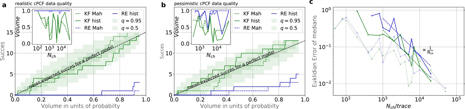
Even for the highest tested experimental noise the RE approach does not follow the required binomial statistics, generating an underestimated uncertainty.

(a) Binomial success statistics of HDCV to cover the true value vs. the expected probability. Calculated for $i = σ$ and $σ_{op} = 0.1 i$ and $λ_{b} = 0.375$ and a strong background noise. (b) Binomial success statistics of HDCV to cover the true value vs. the expected probability. For $10 \cdot i = σ$ and $σ_{op} = 1 i$ and $λ_{b} = 0.375$ and a strong background noise. For both algorithms, the adaptation of the sampler of the posterior was more fragile for small $N_{ch}$ , leading to differences in the posterior if the posterior is constructed from different independent sampling chains. Those data sets were then excluded. We assume that these instabilities are induced in both algorithms by the shortcomings of the multivariate normal assumptions. (c) Comparison of the Euclidean error vs. $N_{ch}$ for the pessimistic noise case (solid lines) with Euclidean error for the optimistic noise case (dotted lines).

Figure 7

Download asset Open asset

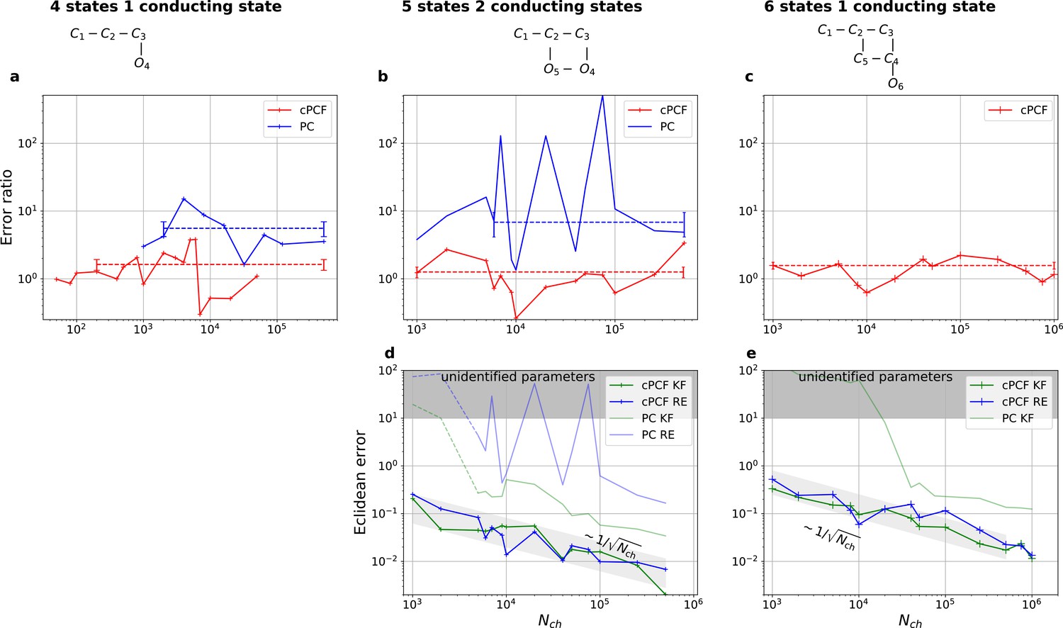
Higher model complexity drastically increases the minimal requirements of the data.

With PC data the RE approach is frequently incapable to identify all parameters while the Bayesian filter is more robust. cPCF data alleviate the parameter unidentifiabilities for patch sizes for which PC data are insufficient. Each panel column corresponds to a particular true process with increasing complexity from left to right, as indicated by the model schemes on top. Within all kinetic schemes, each transition to the right adds one bound ligand. Each transition to left is an unbinding step. Vertical transitions are either conformational or opening transitions. Plots in each row share the same y-axis respectively. Each column shares the same abscissa. (**a-c**) Error ratio for PC data (blue) and cPCF data (red). The dashed lines indicate the mean error ratio under the simplifying assumption that the error ratio does not depend on $N_{ch} .$ The vertical bars are the standard deviations of the mean values. Theses values were calculated from the Euclidean errors shown in Figures 3c and 4a for a, and panels (**d-e**), for (**b-c**), respectively. Results from the KF algorithm (green) and the RE algorithm (blue) are compared for PC (lighter shades) and cPCF (strong lines). The diagonal gray areas indicate a $\sim {(N_{ch})}^{- 0.5}$ proportionality. For simulating the underlying PC data, we used standard deviations of $σ_{op} = 0.1$ and $σ = 1$ and for the cPCF data additionally a ligand of brightness $λ_{b} = 5$ . To facilitate the inference for the two more complex models, we assumed that the experimental noise and the single channel current are well characterized, meaning $i \sim N (i | 1, 0.01)$ , $σ \sim N (σ | 1, 0.01)$ and $σ_{op} \sim gamma (σ_{op} | 1, 100)$ . In the models containing loops (last 2 columns), a prior was used to enforce microscopic-reversibility and set to $k_{25}^{⋆} \sim beta (100, 100)$ multiplied by $k_{1} = k_{5} k_{6} k_{7} k_{8} {(k_{2} k_{3} k_{4})}^{- 1} \cdot 0.995 + 0.01 \cdot k_{1}^{⋆}$ .

Figure 7—source data 1 The folder of the five-state model includes 15 sets of time traces in the interval $N_{ch} \in [10^{3}, 5 \cdot 10^{5}]$ . Each of them has 10 ligand concentrations. The number in the file name reports the amount of ion channels in the patch.: https://cdn.elifesciences.org/articles/62714/elife-62714-fig7-data1-v3.zip
Download elife-62714-fig7-data1-v3.zip
Figure 7—source data 2 The folder of the six-state model includes 14 sets of time traces in the interval $N_{ch} \in [10^{3}, 10^{6}]$ . Each of them has 10 ligand concentrations. The number in the file name reports the amount of ion channels in the patch.: https://cdn.elifesciences.org/articles/62714/elife-62714-fig7-data2-v3.zip
Download elife-62714-fig7-data2-v3.zip

Figure 8

Download asset Open asset

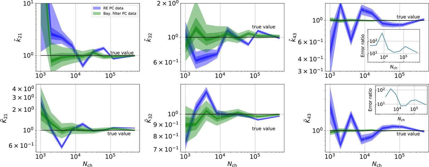
Revisiting the PC data obtained by the 4-state-1-open-state model shows that the KF succeeds to produce realistic uncertainty quantification, while the overconfidence problem (unreliable uncertainty quantification) of the RE approach remains.

Comparison of a series of HDCIs shown as functions of $N_{ch}$ for each parameter of the rate matrix obtained by the KF (green) and the RE algorithm (blue). The differing shades of green and blue indicate the set of $(0.95, 0.6, 0.2, 0.1)$ -HDCIs. Only the interval $N_{c h} > 2 \cdot 10^{3}$ in which all parameters are identified is displayed. The data are taken from the KF vs. RE benchmark of Figures 3c and 7a . The first row corresponds to three rates $k_{i j}$ the second row to the equilibrium constants $K_{i j}$ . All parameters are normalized by their true value. The insets show the error ratios of the respective single parameter estimates. Note that the error ratios on the single-parameter level can be even of the order of magnitude of 10². Thus, they can be much larger than the error ratios calculated from the Euclidean error if the errors of the respective parameters are small compared to other error terms in the Euclidean error Equation 15 .The lowest Euclidean error for this kinetic scheme has cPCF data analyzed with the KF. (Figure 7d). A 6-state-1-open-states model with cPCF data has again an error ratio of the the usual scale (Figure 7c). As expected, the Euclidean error continuously increases with model complexity (Figure 7d and e). For PC data of the 6-state-1-open-states model even the likelihood of the KF is that weak (Figure 7e) that it delivers unidentified parameters even for $N_{ch} = 10^{4}$ and we can detect heavy tailed distributions up until $N_{ch} = 10^{5}$ . Using RE on PC data alone does not lead to parameter identification, thus no error ratio can be calculated.

Figure 9

Download asset Open asset

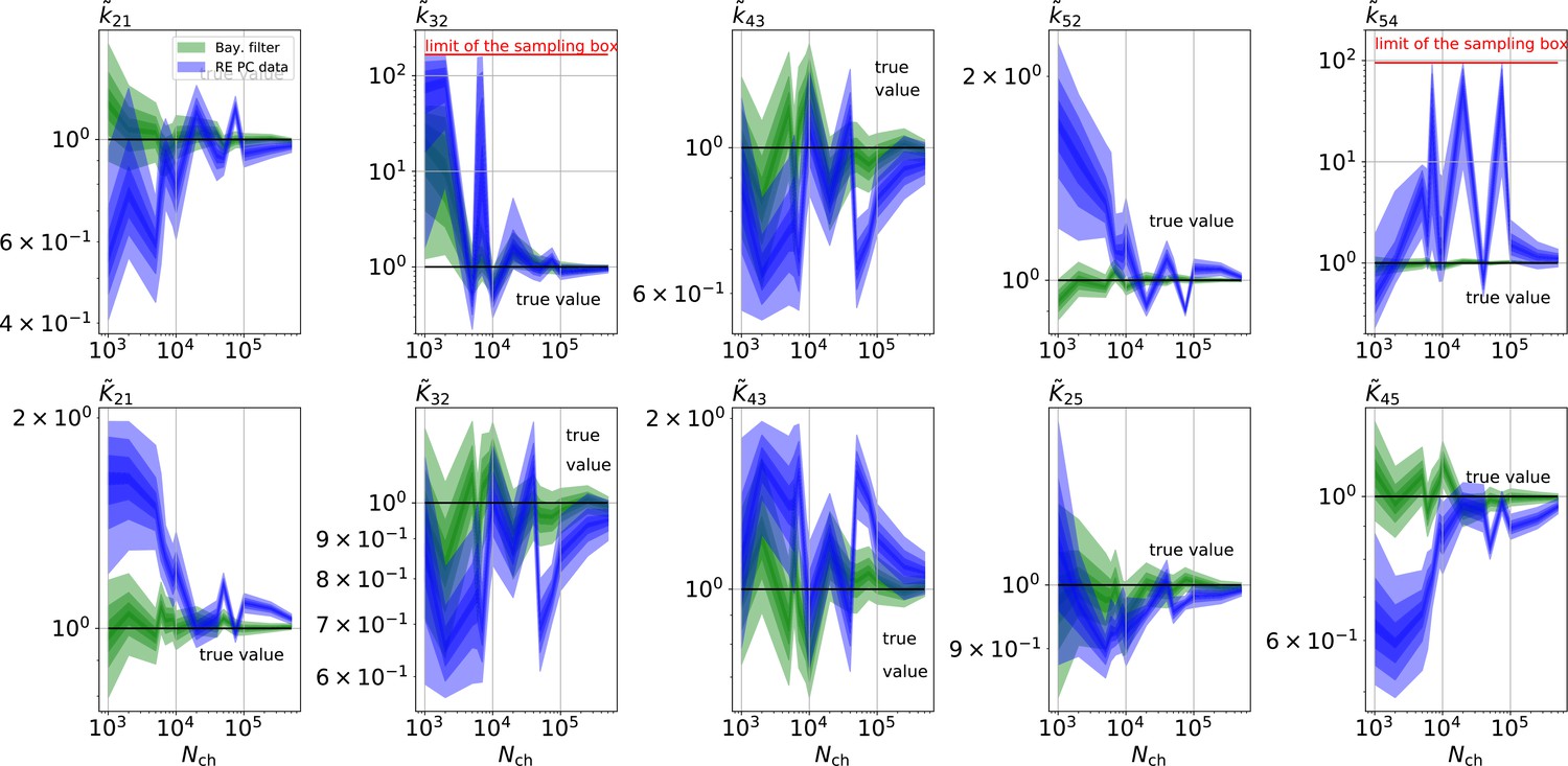
The HDCIs for PC data for a 5-state-2-open-states model show negligible bias for the KF with the true value being included.

In contrast, the HDCE for RE approach frequently does not include the true value and in general appears biased and frequently leaves certain parameters unidentified. Comparison of a series of $(0.95, 0.6, 0.2, 0.1)$ -HDCIs as functions of $N_{ch}$ for each parameter of the rate matrix obtained by the KF (green) and the RE algorithm (blue). The HDCIs correspond to the PC data displayed in Figure 7b and d . The first row corresponds to three rates $k_{i j}$ the second row to the equilibrium constants $K_{i j}$ . All parameters are normalized by their true value. ${\tilde{K}}_{25}$ is because of the microscopic-reversibility prior a parameter which is strongly dependent on the other rates and ratios. Refer to the caption of Figure 7 for details about the prior that enforces microscopic-reversibility. Thus, the deviations of ${\tilde{K}}_{25}$ are inherited from the other parameters. The rate ${\tilde{k}}_{54}$ is frequently not identified by the RE approach and only the limits of the sampling box confines he posterior.

Figure 10

Download asset Open asset

The Benchmark of the KF for PC versus cPCF data with different bright ligands shows that even adding a weak fluorescence binding signal can add enough information to identify before unidentified parameters.

(a) Posteriors of PC data (blue), cPCF data with $λ_{b} = 0.00375$ (orange) and cPCF data with $λ_{b} = 0.375$ (green). For the data set with $λ_{b} = 0.375$ , we additionally accounted for the superimposing fluorescence of unbound ligands in solution. In all cases $N_{ch} = 10^{3}$ . The black lines represent the true values of the simulated data. The posteriors for cPCF $ℙ (k_{2, 1}, k_{3, 2})$ are centered around the true values that are hardly visible on the scale of the posterior for the PC data. The solid lines on the diagonal are kernel estimates of the probability density. (b) Accuracy and precision of the median estimates visualized by a violin plot for the parameters of the rate matrix for 5different data sets. Four of the five data sets are used a second time with different instrumental noise, with $λ_{b} = 0.375$ and superimposing bulk signal. The blue lines represent the median, mean and the maximal and minimal extreme value. (c) The 95th percentile of the marginalized posteriors vs. $λ_{b}$ normalized by the true value of each parameter. A regime with $l_{95} \sim 1 / \sqrt{λ}$ is shown for $k_{2, 1}$ and K₁, while other parameters show a weaker dependency on the ligand brightness. (d) Histograms of the residuals $r$ of cPCF with $λ_{b} = 2.5 \cdot 10^{- 3}$ data and PC data. The randomness of the normalized residuals of the cPCF or PC data is well described by $r_{i} \sim normal (0, σ_{res}^{2} = 1)$ . The estimated variance is $σ_{res}^{2} = 0.98 + 0.26$ . Note that the fluorescence signal per frame is very low such that the normal approximation to Poisson counting statistics does not hold. e, Posterior of the open-channel noise $ℙ (σ_{op}^{2} / σ_{op, true}^{2})$ for PC data with $N_{ch} = 10^{3}$ (green) and $N_{ch} = 10^{5}$ (blue) as well as for cPCF data with $N_{ch} = 10^{3}$ (red) with $λ_{b} = 0.375$ . We assumed as prior for the instrumental variance $P (σ^{2}) = N (1, 0.01)$ .

Figure 10—source data 1 Five different sets of time traces of panel b. All instrumental noise is already added.: https://cdn.elifesciences.org/articles/62714/elife-62714-fig10-data1-v3.zip
Download elife-62714-fig10-data1-v3.zip
Figure 10—source data 2 Eighteen sets of time traces of panel c. The number in the file name indicates the brightness.: https://cdn.elifesciences.org/articles/62714/elife-62714-fig10-data2-v3.zip
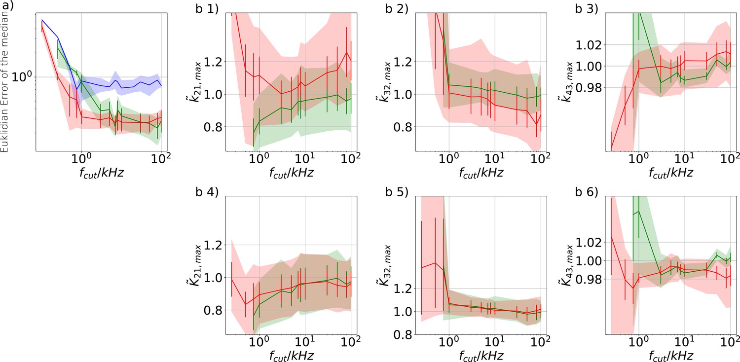
Download elife-62714-fig10-data2-v3.zip

Figure 11

Download asset Open asset

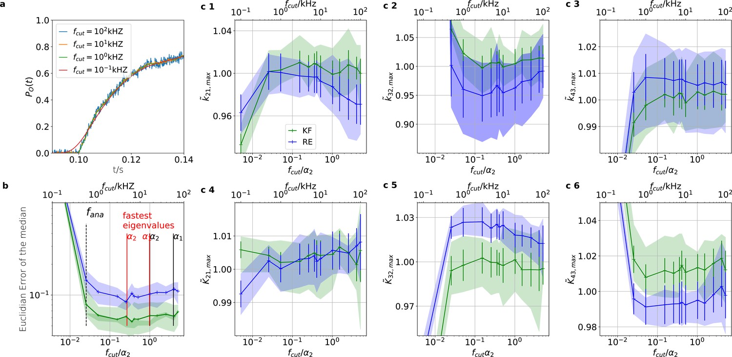
The KF is robust against moderate analog filtering of the current signal.

High (Bayesian) sampling frequencies and minimal analog filtering does minimize bias which otherwise deteriorates parameter identification. In order to mimic an analog signal before the analog-to-digital conversion we simulated seven different 100 kHz signals which were then filtered by a digital fourth-order (4 pole) Bessel filter. The activation curves were then analyzed with the Bayesian filter at 125 Hz and the deactivation curves at sampling rates between 166-500 Hz. We chose for the analog signal $σ_{\exp} / i = 10$ , $σ_{op} / i = 0.1$ , thus a stronger background noise, and we set the mean photon count per bound ligand as $λ_{b} = 5$ . For the ensemble size we choose $N_{ch} = 10^{3}$ . (a) Current time trace filtered with different f_cut. Except for 100 Hz (red) the signal distortion is visually undetectable. Nevertheless, the invisible signal distortions from analog filtering are problematic for both algorithms. (b) Estimate of the distribution mean Euclidean error of the median of the posterior vs. the cut-off frequency of a 4 pole Bessel filter (upper scale is in units of kHz) or scaled to the channel time scale (lower scale, see text). The fastest two eigenvalues $α_{1, 2} / α_{2}$ for the highest ligand concentration are indicated by the black vertical lines. The fastest ratios $α_{1, 2} / α_{2}$ for the next smaller ligand concentration are indicated by the red vertical lines. The slowest eigenvalue ratio $α_{3} / α_{2}$ at the highest ligand concentration is beyond the left limit of the x-axis. The solid line is the mean median of five data sets of the respective RE posterior (blue) and KF posterior (green). The green shaded area indicates the 0.6 quantile (ranging from the 20th percentile till the 80th percentile), demonstrating the distribution of the error of the posterior median due to the randomness of the data. (c) 1–3, Accuracy (bias) and precision of the maxima of the posterior ${\tilde{k}}_{\max, i j}$ of the posterior maxima of the rates vs. the cut-off frequency of a Bessel filter. The shaded areas indicate the 0.6 quantiles (ranging from the 20th percentile till the 80th percentile) due the variability among data sets while the error bars show the standard error of the mean. The deviation of the mean from the true value is an estimate of the accuracy of the algorithm while the quantile indicates the precision. (c) 4–6, Accuracy and precision of the maxima of the posterior ${\tilde{K}}_{\max, i j}$ of the posterior maxima of the corresponding equilibria vs. the cut-off frequency of a Bessel filter.

Figure 11—source data 1 Representative data set of cPCF data whose current has been filtered with decreasing f_cut. In the name of each file is f_cut encoded in units of 100 kHz. The time axis is identical for all time traces and saved in the file Time.txt. The folder is similar to six other provided source data folders which have in total been used in this figure.: https://cdn.elifesciences.org/articles/62714/elife-62714-fig11-data1-v3.zip
Download elife-62714-fig11-data1-v3.zip
Figure 11—source data 2 Representative data set of cPCF data whose current has been filtered with decreasing f_cut.: https://cdn.elifesciences.org/articles/62714/elife-62714-fig11-data2-v3.zip
Download elife-62714-fig11-data2-v3.zip
Figure 11—source data 3 Representative data set of cPCF data whose current has been filtered with decreasing f_cut.: https://cdn.elifesciences.org/articles/62714/elife-62714-fig11-data3-v3.zip
Download elife-62714-fig11-data3-v3.zip
Figure 11—source data 4 Representative data set of cPCF data whose current has been filtered with decreasing f_cut.: https://cdn.elifesciences.org/articles/62714/elife-62714-fig11-data4-v3.zip
Download elife-62714-fig11-data4-v3.zip
Figure 11—source data 5 Representative data set of cPCF data whose current has been filtered with decreasing f_cut.: https://cdn.elifesciences.org/articles/62714/elife-62714-fig11-data5-v3.zip
Download elife-62714-fig11-data5-v3.zip
Figure 11—source data 6 Representative data set of cPCF data whose current has been filtered with decreasing f_cut.: https://cdn.elifesciences.org/articles/62714/elife-62714-fig11-data6-v3.zip
Download elife-62714-fig11-data6-v3.zip

Figure 12

Download asset Open asset

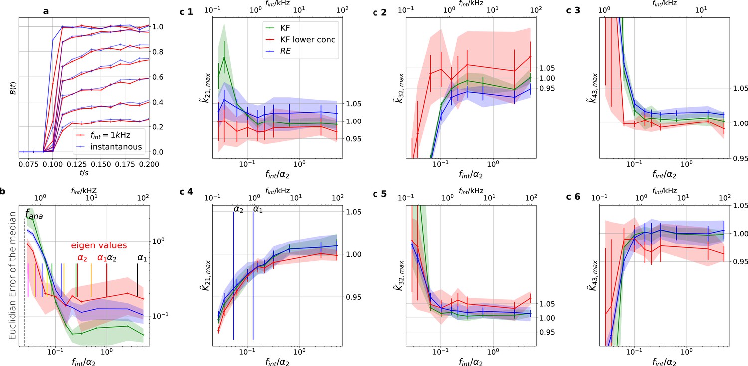
Finite integration time of fluorescence recordings acts also as a filter.

Thus the sampling should be faster than the fastest eigenvalues to avoid biased results. We simulated five different 100 kHz cPCF signals. All forms of noise were added and then the fluorescence signal was summed up using a sliding window to account for the integration time to produce one digital data point. The activation curves were then analyzed with the Bayesian filter at 125 Hz and the deactivation curves at $166 - 500$ kHz, see caption of Figure 8. We plot the 0.6-quantile (interval between the 20th and the 80th percentile) to mimic ±one standard deviation from the mean as well as the mean of the distribution of the maxima of the posterior for different data sets. (Note, this is not equivalent to the mean and quantiles of the posterior of a single data set.). The quantiles represent the randomness of the data while the error bars indicate the standard error of the mean maximum of the posterior. Blue (RE) and green (KF) indicate the two algorithms with the standard data set while red (KF) shows examples that use only the six smallest ligand concentrations for the analysis in order to limit the highest eigenvalues. a, Instantaneous probing of the ligand binding (blue) compared with a probing signal which runs at $f_{int} = 1$ kHz. The integrated brightness of the bound ligand is $λ_{b} = 5$ photons per frame. Although the red curves seem like decent measurements of the process except for the highest two shown ligand concentrations, the mean error is roughly an order of magnitude worse than for $f_{int} = 10$ kHz. Note, that for visualization we plot at a higher frequency than the Kalman filter analyzed the data. b, Estimate of the distribution of the (Euclidean error of the mean median of the posterior) vs. the scaled integration frequency $f_{int} / α_{2} = 1 / (α_{2} \cdot T_{integration})$ . We use integration frequency instead of the integration time to make the plot comparable to the Bessel filter plot. The solid line is the mean median of five data sets of the respective KF posterior (green, red) and RE posterior (blue). The shaded areas indicate the 0.6-quantile which visualizes the spread of the distribution of point estimates. The two fastest time scales (eigenvalues) at the highest ligand concentration are indicated by the vertical black lines, the time scales of the next lower ligand concentrations with the red vertical lines. c 1–3, Accuracy (bias) and precision of the maxima of the posterior $k_{i j, m a x}$ rates vs. the integration frequency. c 4–6, Accuracy and precision of the maxima of the posterior $K_{i j, m a x}$ of the corresponding equilibria vs. the cut-off frequency of a Bessel filter.

Figure 12—source data 1 The data folder contains one data set of cPCF data. The fluorescence has been integrated with decreasing f_int. The number in the file name encodes the amount of $100 k H z$ data points which have been summed up to mimic the integration time. The time axis is identical for all time traces and saved in the file Time.txt. The folder is similar to six other provided source data folders which have in total been used in this figure.: https://cdn.elifesciences.org/articles/62714/elife-62714-fig12-data1-v3.zip
Download elife-62714-fig12-data1-v3.zip
Figure 12—source data 2 The data folder contains one data set of cPCF data.: https://cdn.elifesciences.org/articles/62714/elife-62714-fig12-data2-v3.zip
Download elife-62714-fig12-data2-v3.zip
Figure 12—source data 3 The data folder contains one data set of cPCF data.: https://cdn.elifesciences.org/articles/62714/elife-62714-fig12-data3-v3.zip
Download elife-62714-fig12-data3-v3.zip
Figure 12—source data 4 The data folder contains one data set of cPCF data.: https://cdn.elifesciences.org/articles/62714/elife-62714-fig12-data4-v3.zip
Download elife-62714-fig12-data4-v3.zip
Figure 12—source data 5 The data folder contains one data set of cPCF data.: https://cdn.elifesciences.org/articles/62714/elife-62714-fig12-data5-v3.zip
Download elife-62714-fig12-data5-v3.zip
Figure 12—source data 6 The data folder contains one data set of cPCF data.: https://cdn.elifesciences.org/articles/62714/elife-62714-fig12-data6-v3.zip
Download elife-62714-fig12-data6-v3.zip
Figure 12—source data 7 The data folder contains one data set of cPCF data.: https://cdn.elifesciences.org/articles/62714/elife-62714-fig12-data7-v3.zip
Download elife-62714-fig12-data7-v3.zip

Appendix 1—figure 1

Download asset Open asset

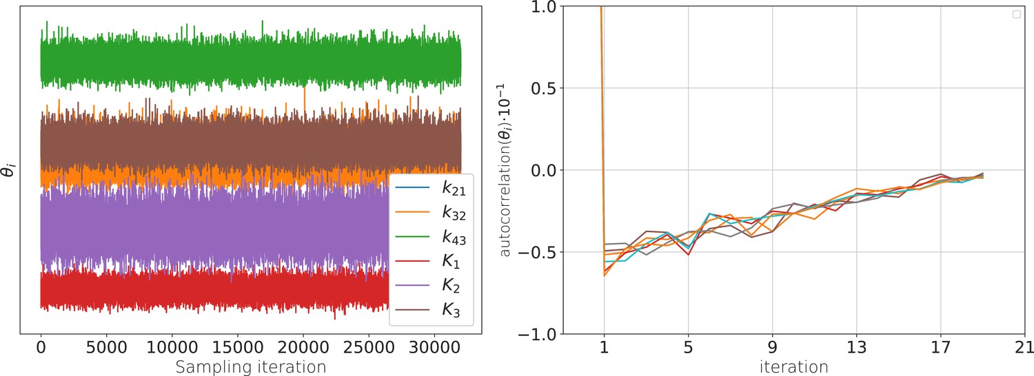
The posterior samples display autocorrelation which lowers the effective sample size.

(a) Sample traces from the 6-dimensional posterior of the rate matrix recorded after the warm-up of the sampler. (b) These traces are anti-correlated (in time) such that the effective sample size with which all quantities of relevance are estimated is smaller than the actual number of samples. Note that even at one iteration the absolute value of the auto-correlation is never larger than 0.05. The standard error of the bootstrapped mean auto-correlation is in the order of $10^{- 4}$ .

Appendix 1—figure 2

Download asset Open asset

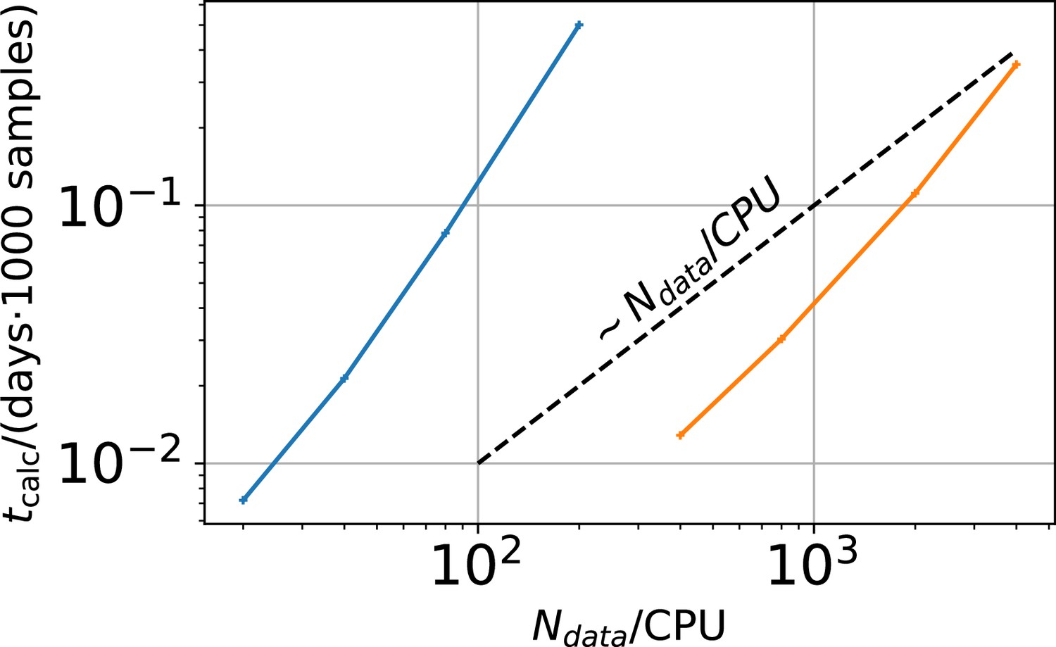
Computational time in units of 1000 samples per day vs $N_{data} / CPU$ $10^{- 4}$ .

The two colors represent two different implementations. The difference between the two implementations is that the derived quantities which are the predicted mean signal and the predicted signal variance for each data point in the less efficient sampling algorithm are saved. In the more efficient algorithm these derived quantities are discarded.

Appendix 1—figure 3

Download asset Open asset

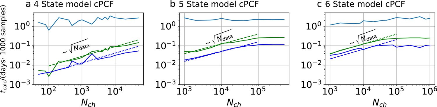
Computational time for cPCF data.

Computational time in units of 1000 samples per day vs. the amount of ion channels per trace $N_{ch}$ . The green curve belongs to the results from the KF, the blue curve to the results from the RE approach. The brighter blue curve corresponds to the ratio of computational time. a, four-state model with cPCF data. The posterior of the RE approach was sampled from three independent chains. We drew 18,000 samples per chain which included a large fraction of 6000 warm-up samples per chain. The posterior of the KF was sampled from 4independent chains. We drew 26,000 samples per chain which included a large fraction of 4000 warm-up samples per chain. b Computational time of the 5-state-2-open-states model with cPCF data. The KF algorithm drew 9000 samples which included a large fraction of 6,000 warm-up samples per chain. The RE algorithm drew 10,000 samples which included a large fraction of 5,000 warm-up samples per chain. In total, we used four independent chains. c, Computational time of the 6-state-1-open-state model with cPCF data. The KF algorithm drew 10,000 samples which included a large fraction of 6000 warm-up samples per chain. The RE algorithm drew 12,000 samples which included a large fraction of 7000 warm-up samples per chain. In total, we used four independent sampling chains.

Appendix 1—figure 4

Download asset Open asset

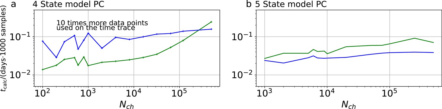
Computational time for PC data.

The computational time in units of 1,000 samples per day are plotted vs the amount of ion channels per trace $N_{ch}$ . The green curve belongs to the results from the KF, the blue curve to the results from the RE approach. a, Four-state model with PC data. In contrast to the cPCF data (Appendix 1—figure 3), f_ana is increased by an order of magnitude. Thus, 10 times more data points per time trace and CPU are evaluated. These results were obtained by four independent chains which drew 9000 samples per chain, including a large fraction of 7000 warm-up samples per chain.b, Five-state model with PC data. Note that here f_ana equals the analyzing frequency of cPCF data (Appendix 1—figure 3).

Appendix 5—figure 1

Download asset Open asset

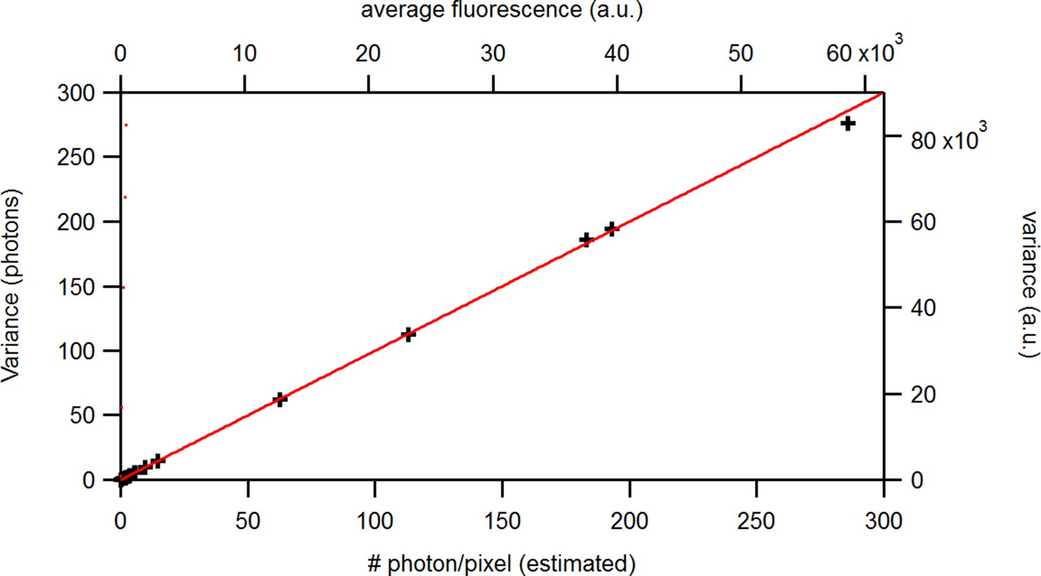
Benchmark of the signal variance vs its mean for experimental solution data recorded under cPCF conditions: The concentrations of the fluorescent ligand were 0.25, 3, and 15 $μ M$ and a reference dye was present. The laser intensities covered 1.6 orders of magnitude at constant detection settings. The data points were obtained from $1.4 \cdot 10^{6} pixel$ . The red and blue lines indicate the theoretical prediction for a Poisson and Gamma distribution, respectively, assuming $θ = 1$ . The linear relation allows to relate the measured a.u. (top, right axis) to photons (bottom, left axis). The inset provides the corresponding log-log plot. Important for the KF algorithm is that skewness and excess kurtosis is small.

Appendix 5—figure 2

Download asset Open asset

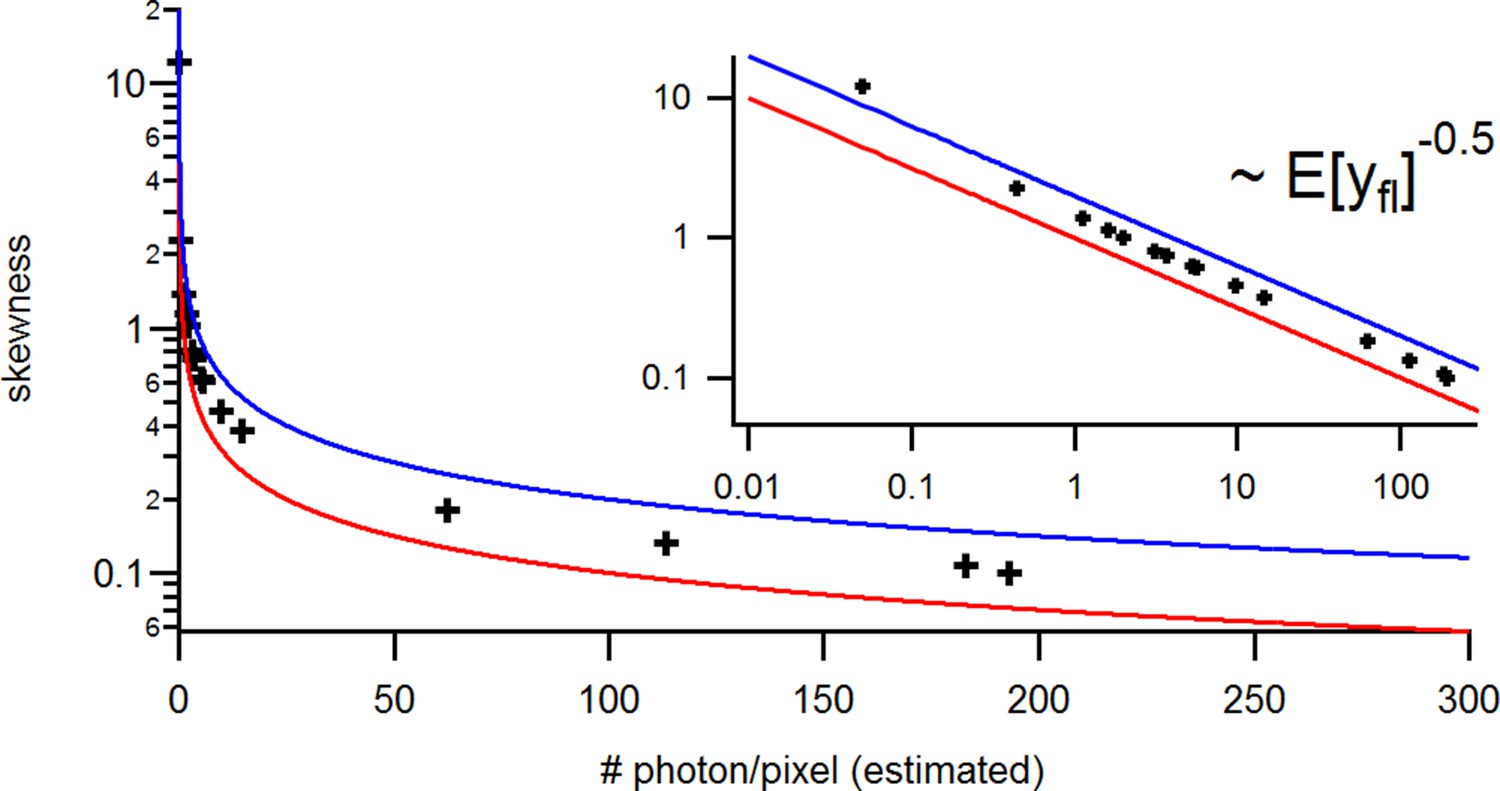
Benchmark of the signal Skewness vs its the mean for the identical experimental solution data under cPCF conditions.

The Skewness is small but the values are slightly larger than theoretically predicted. The inset provides the corresponding log-log plot. Important for the KF algorithm is that skewness and excess kurtosis is small.

Appendix 5—figure 3

Download asset Open asset

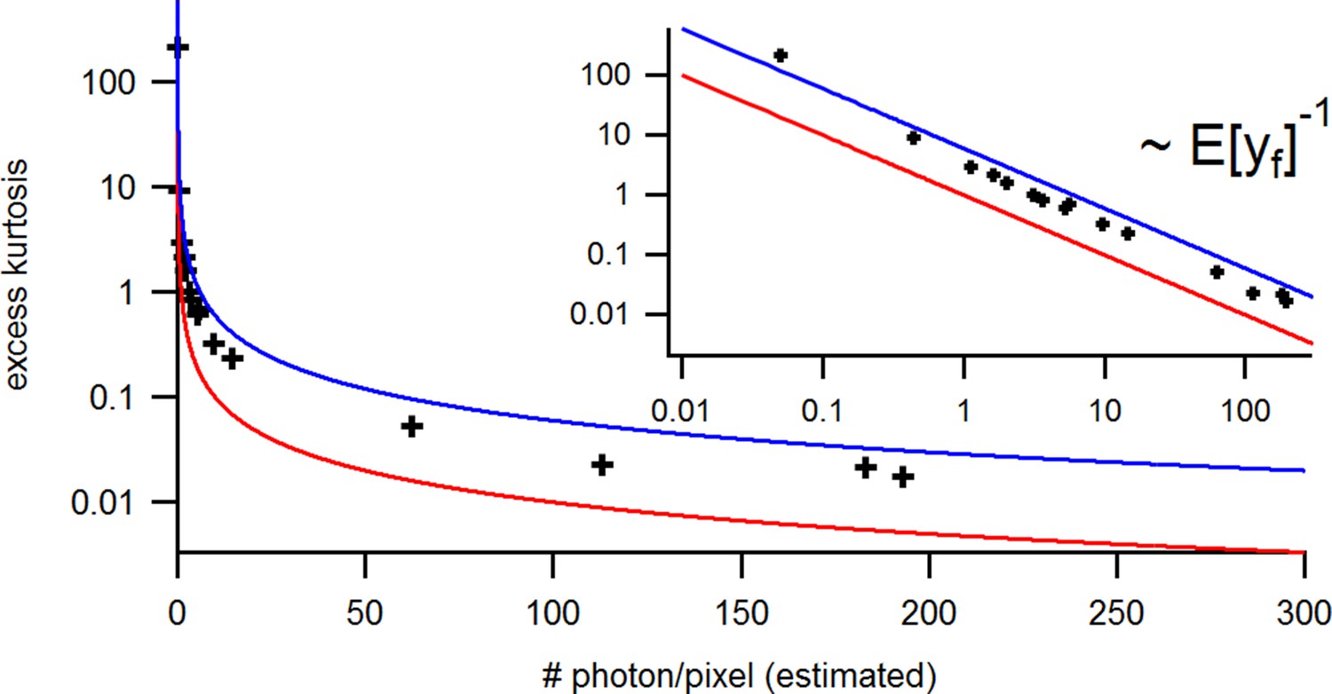
Benchmark of the signal Kurtosis vs its mean for the identical experimental solution data under cPCF conditions.

The Kurtosis is small but the values are slightly larger than theoretically predicted. The inset provides the corresponding log-log plot. Important for the KF algorithm is that skewness and excess kurtosis is small.

Appendix 5—figure 4

Download asset Open asset

Simulated binding signals.

a, Comparison of binding of a labeled ligand at two concentrations. A simple two-ligand binding process was simulated with the Hill equation for the two expression levels of 1000 or 10,000 binding sites per patch and a BC₅₀ of 1000 (BC₅₀a) or 10,000(BC₅₀b), respectively, given in molecules per observation unit. The observed signal is the sum of the signal from ligands free in solution and bound to the receptors. The solution signal scales linearly with the concentration, while the binding signal saturates.

Appendix 5—figure 5

Download asset Open asset

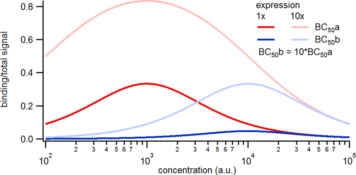
Simulated binding signals.

Relative contribution of the binding signal to the total signal. Note that the contribution of the binding signal scales linearly with the expression level and inversely with the. $B C_{50}$

Appendix 5—figure 6

Download asset Open asset

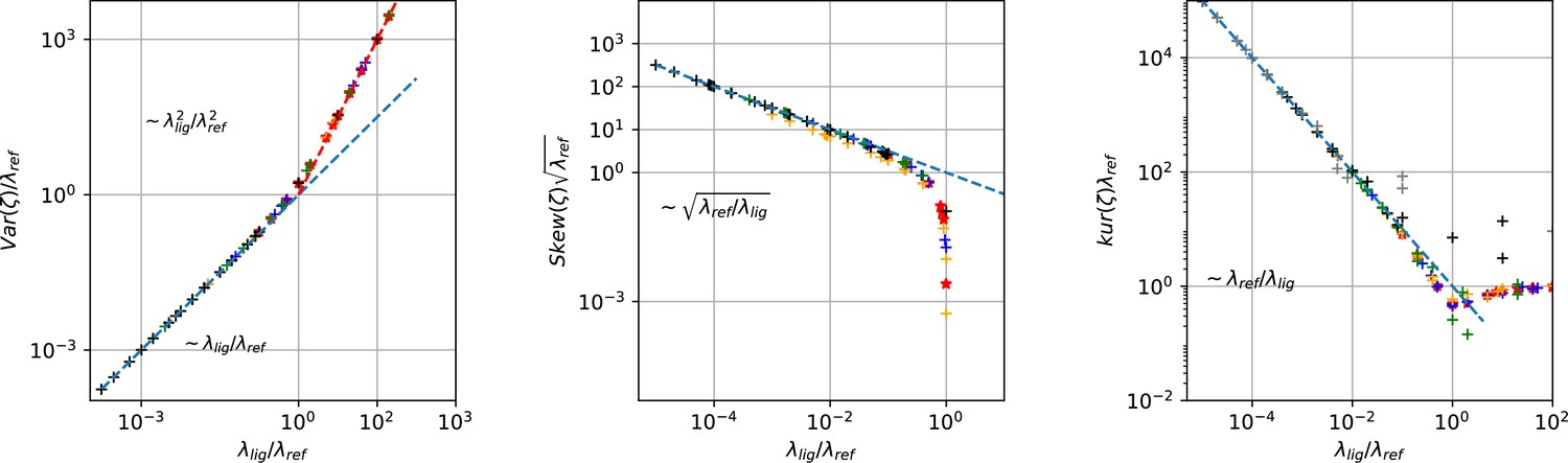
Master curves of 2nd till 4th centralized moment of photon counting noise ζ arising from the difference signal of fluorescent ligands and the dye in the bulk.

The curves are created from $4 \cdot 10^{5}$ draws from Poisson distributions with different combinations of intensities for the reference dye $λ_{ref}$ and of the intensity of the confocal voxel fraction. $λ_{lig}$

Appendix 7—figure 1

Download asset Open asset

Influence of analog filtering on the accuracy and precision of the maximum of the posterior from PC data We chose for the analog signal $σ_{\exp} / i = 10$ , $σ_{op} / i = 0.1$ , thus a strong background noise.

For the ensemble size, we chose $N_{ch} = 4 \cdot 10^{3}$ such that the likelihood dominates the uniform prior. (a) Estimate of the distribution of the accuracy (mean Euclidean error of the median of the posterior) vs. the cut-off frequency of a 4th-order Bessel filter scaled to the channel time scale. The solid line is the mean median of 5 data sets of the respective RE posterior (blue) and KF posterior (green). The green shaded area indicates the 0.6 quantile (ranging from 0.2 till 0.8) demonstrating the distribution of the error of the median of the posterior due to the randomness of data.(b 1–3) Accuracy and precision of the maxima of the posterior ${\tilde{k}}_{i j, m a x}$ of the maxima of the posterior rates vs. the cut-off frequency of a Bessel filter. The shaded areas indicate the 0.6 quantiles (ranging from 0.2 till 0.8) due to the variability from data set do data set while the error bars show the standard error of the mean. (b 4–6) Accuracy and precision of the maxima of the posterior ${\tilde{K}}_{i j, m a x}$ of the maxima of the posterior of the corresponding equilibria vs. the cut-off frequency of a Bessel filter.

Appendix 9—figure 1

Download asset Open asset

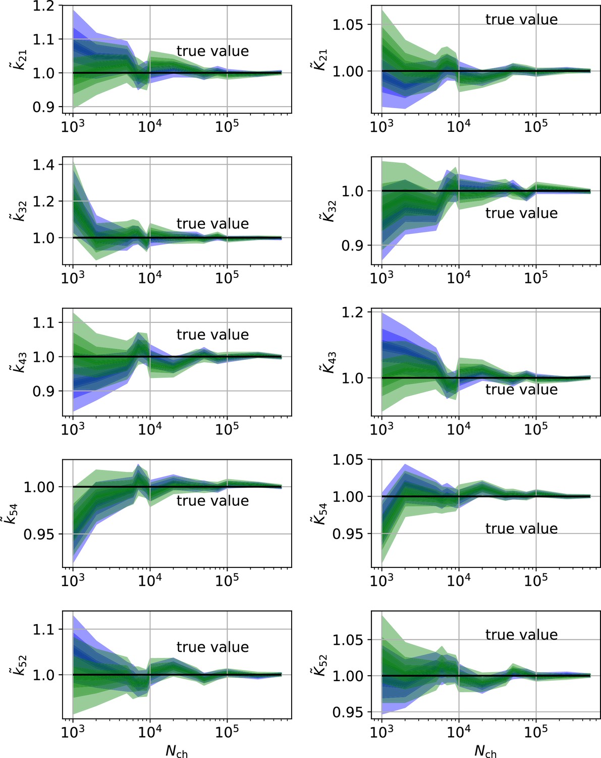
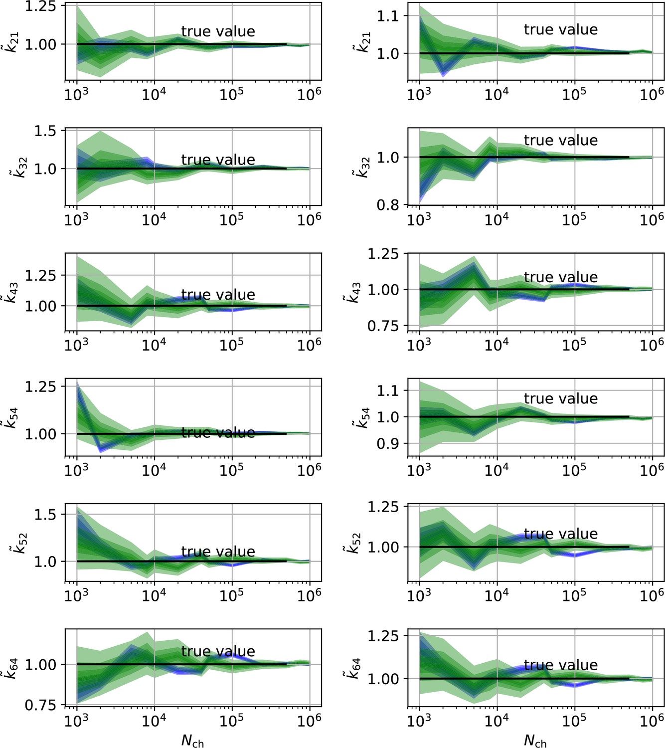
HDCIs vs $N_{ch}$ for the 5-state-2-open-states model for cPCF data.

The single parameter level corresponds to the Euclidean error of Figure 7d. Compared to the main text we switched rows with columns of the panels, the first column represents now the rates and the second column the equilibrium constants. The prior that enforces microscopic-reversibility is identical to the prior mentioned in the caption of Figure 7.

Appendix 9—figure 2

Download asset Open asset

HDCIs vs $N_{ch}$ for the 6-states-1-open-state model for cPCF data.

The single parameter level corresponds to the Euclidean error of Figure 7e. Compared to the main text we switched rows with columns of the panels, the first column represents now the rates and the second column the equilibrium constants. The prior that enforces microscopic-reversibility is identical to the prior mentioned in the Figure 7.

Tables

Table 1

Important symbols.

Symbol	Meaning
$θ$	Set of all unknown model parameters for which the posterior distribution is sampled
$n (t)$	Hidden ensemble occupancy vector of channel states in a specific patch at time $t$ which is a continuous Markov state vector $n (t) \in R^{M}$
$P (t)$	Variance-covariance matrix of a hidden ensemble state $n (t)$ n a specific patch at time $t$ which contains the dispersion of the ensemble and the lacking knowledge of the algorithm about the true $n (t)$
$T$	Transition matrix of a single channel
$K$	Rate matrix which is the logarithm of the transition matrix
$H$	Observation matrix which projects the hidden ensemble state vector onto its mean signal.
$s$	Single-molecule Markov state vector
$k_{i, j}$	Specific transition rate from state j to state i, $[K]_{i, j} = k_{i, j}$ ,
$K_{i}$	Ratio of two transition rates i.e. an equilibrium constant
$y (t)$	Data point at time
$T$	Number of observations in a time series
$Y_{T}$	Time series of $T$ data points, $Y_{T} = {y (t_{i})}_{i = 1}^{T}$
$N_{T}$	Time series of $T$ hidden ensemble states, $N_{T} = {n (t_{i})}_{i = 1}^{T}$
$N_{ch, j}$	Number of channels in patch number
$i$	Mean electrical current through a single-channel
$σ_{m}^{2}$ and $σ_{e x}^{2}$	Variance of the current including all noise from the patch and the recording system
$σ_{op}^{2}$	Variance of the current noise generated by a single open-channel
$λ_{b}$	Mean brightness of a bound ligand
$λ_{Fl}$	Mean brightness of the fluorescence signal from bulk and bound ligands
$σ_{b a c k}^{2}$	Variance of the fluorescence generated by unbound ligands after subtraction of the image obtained for the reference dye
$M$	Number of single-channel states which is the dimension of $n (t) \in N^{M}$ in the KF algorithm
$N_{o b s}$	Dimensions of the observational space
$F (Y)$	True probability density of $Y$ , i.e. the true data-generating process
$L (Y \| θ)$	Likelihood function of the model parameters
$P (θ \| Y)$	Posterior distribution of the model parameters
$P_{p r e d} (\tilde{Y} \| Y)$	Predictive distribution of the new data points
$O (y \| n)$	Distribution of observables for a single time step
$N (\cdot \| μ, Σ)$	Normal distribution with mean μ and variance-covariance matrix $\sum$
$E [\cdot]$	Mean value

Table 2

Summary of signals and noise sources for the exemplary CCCO model with the closed states $α = 1, 2, 3$ and the open state $α = 4$ .

The observed space is two-dimensional with $y_{F l} = fluorescence$ and $y_{I} = ion current$ . The fluorescence signal is assumed to be derived from the difference of two spectrally different Poisson distributed fluorescent signals. That procedure results in a scaled Skellam distribution of the noise.

	ion current		fluorescence
	current signal	measurement noise	fluorescence signal	background fluorescence
Signaling states	Open state	-	Ligand-bound states	-
Error term	Open-channel noise	Measurement noise	Photon counts	Bulk noise
Affected signal	Current	Current	Fluorescence	Fluorescence
Distribution	Normal $(i n_{4}, σ_{o p}^{2} n_{4})$	Normal $(0, σ_{m}^{2})$	Poisson $(λ_{b} n_{i} (t))$	Scaled Skellam
Contribution to $H$	$H_{2, 4} = i$	-	$H_{1, :} = (0, λ_{b}, 2 λ_{b}, 2 λ_{b})$	-
Contribution to $Σ$	$Σ_{2, 2} = σ_{op}^{2} n_{4} (t)$	$Σ_{2, 2} = σ_{m}^{2}$	$Σ_{1, 1} = (0, λ_{b}, 2 λ_{b}, 2 λ_{b}) n (t)$	$Σ_{1, 1} = σ_{back}^{2}$

Appendix 1—table 1

Typical summary statistics of the posterior as printed by the “summary” method from the “fit” object in Pystan.

We deleted the 25% and 75% percentiles to decrease the size of the table and changed some of the names with respect to the used name in the algorithm to the symbol used in this article. Note that we assumed to measure 2 ligand concentrations (which includes 4 jumps) from one patch. Thus, we assumed for 10 ligand concentrations that they are coming from 5 patches which leads to a five-dimensional channels per patch vector $N_{ch}$ . The bias of $N_{ch}$ $i$ discussed in the main article, is also observed here.

	mean	se_mean	sd	2.5%	50%	97.5%	n_eff	Rhat
k₂₁	507.65	0.06	11.91	484.74	507.46	531.62	41262	1.0
k₃₂	481.15	0.16	28.63	428.34	480.19	540.32	33610	1.0
k₄₃	509.95	0.04	6.99	496.39	509.91	523.77	36006	1.0
K₁	0.5	2.6e-5	5.2e-3	0.49	0.5	0.51	40548	1.0
K₂	0.51	6.7e-5	0.01	0.49	0.51	0.54	33228	1.0
K₃	0.49	4.2e-5	7.5e-3	0.47	0.49	0.5	31445	1.0
N_ch[1]	1007.1	0.14	20.05	968.84	1006.8	1047.2	19838	1.0
N_ch[2]	1006.1	0.14	20.04	967.83	1005.8	1046.0	19874	1.0
N_ch[3]	1003.9	0.14	20.0	965.66	1003.6	1043.8	19877	1.0
Nch[4]	1007.0	0.14	20.09	968.67	1006.6	1047.1	19843	1.0
N_ch[5]	1005.9	0.14	20.09	967.61	1005.6	1045.9	19874	1.0
i	1.0	7.0e-5	9.8e-3	0.98	1.0	1.02	19971	1.0
$σ_{\exp}^{2}$	0.25	1.2e-5	2.5e-3	0.25	0.25	0.26	43142	1.0
$σ_{op}^{2}$	2.5e-3	1.2e-7	2.5e-5	2.5e-3	2.5e-3	2.5e-3	42707	1.0
$σ_{fluo}^{2}$	1.3e-5	2.3e-8	4.6e-6	1.0e-5	1.2e-5	2.5e-5	41306	1.0
λ	9.98	1.1e-4	0.02	9.94	9.98	10.02	35109	1.0

Additional files

Transparent reporting form: https://cdn.elifesciences.org/articles/62714/elife-62714-transrepform1-v3.docx
Download elife-62714-transrepform1-v3.docx
Source code 1 cPCF data simulation code.: https://cdn.elifesciences.org/articles/62714/elife-62714-code1-v3.zip
Download elife-62714-code1-v3.zip

Download links

A two-part list of links to download the article, or parts of the article, in various formats.

Downloads (link to download the article as PDF)

Article PDF

Open citations (links to open the citations from this article in various online reference manager services)

Mendeley

Cite this article (links to download the citations from this article in formats compatible with various reference manager tools)

Jan L Münch
Fabian Paul
Ralf Schmauder
Klaus Benndorf

(2022)

Bayesian inference of kinetic schemes for ion channels by Kalman filtering

eLife 11:e62714.

https://doi.org/10.7554/eLife.62714

Share this article

Cite this article

The First-order Markov property of the data requires a recursive prediction of the signal (by the model) and correction (by the data) scheme of the algorithm.

The residuals between model prediction and data reveal long autocorrelations if the analysis algorithm ignores the first-order Markov property.

Kinetic scheme and simulated data.

Figure 1—source data 1

The first-order hidden Markov structure is explicitly used by the Bayesian filter.

The Bayesian filter overcomes the sensitivity to varying (open-channel) noise of the classic Kalman filter and does not show the overconfidence of the RE-approach.

Figure 3—source data 1

For multidimensional data (cPCF) the RE approach almost approaches the accuracy (Euclidean error) of the Bayesian Filter.

Figure 4—source data 1

Figure 4—source data 2

Figure 4—source data 3

Figure 4—source data 4

Figure 4—source data 5

Figure 4—source data 6

Figure 4—source data 7

Figure 4—source data 8

Figure 4—source data 9

Figure 4—source data 10

Figure 4—source data 11

Figure 4—source data 12

The HDCV of the posterior of the KF follows the requested binomial statistics while the HDCVs of the RE approach are too narrow.

Even for the highest tested experimental noise the RE approach does not follow the required binomial statistics, generating an underestimated uncertainty.

Higher model complexity drastically increases the minimal requirements of the data.

Figure 7—source data 1

Figure 7—source data 2

Revisiting the PC data obtained by the 4-state-1-open-state model shows that the KF succeeds to produce realistic uncertainty quantification, while the overconfidence problem (unreliable uncertainty quantification) of the RE approach remains.

The HDCIs for PC data for a 5-state-2-open-states model show negligible bias for the KF with the true value being included.

The Benchmark of the KF for PC versus cPCF data with different bright ligands shows that even adding a weak fluorescence binding signal can add enough information to identify before unidentified parameters.

Figure 10—source data 1

Figure 10—source data 2

The KF is robust against moderate analog filtering of the current signal.

Figure 11—source data 1

Figure 11—source data 2

Figure 11—source data 3

Figure 11—source data 4

Figure 11—source data 5

Figure 11—source data 6

Finite integration time of fluorescence recordings acts also as a filter.

Figure 12—source data 1

Figure 12—source data 2

Figure 12—source data 3

Figure 12—source data 4

Figure 12—source data 5

Figure 12—source data 6

Figure 12—source data 7

The posterior samples display autocorrelation which lowers the effective sample size.

Computational time in units of 1000 samples per day vs Ndata/CPU10-4.

Computational time for cPCF data.

Computational time for PC data.

Benchmark of the signal Skewness vs its the mean for the identical experimental solution data under cPCF conditions.

Benchmark of the signal Kurtosis vs its mean for the identical experimental solution data under cPCF conditions.

Simulated binding signals.

Simulated binding signals.

Master curves of 2nd till 4th centralized moment of photon counting noise ζ arising from the difference signal of fluorescent ligands and the dye in the bulk.

Influence of analog filtering on the accuracy and precision of the maximum of the posterior from PC data We chose for the analog signal σexp/i=10, σop/i=0.1, thus a strong background noise.

HDCIs vs Nch for the 5-state-2-open-states model for cPCF data.

HDCIs vs Nch for the 6-states-1-open-state model for cPCF data.

Important symbols.

Summary of signals and noise sources for the exemplary CCCO model with the closed states α=1,2,3 and the open state α=4.

Typical summary statistics of the posterior as printed by the “summary” method from the “fit” object in Pystan.

Transparent reporting form

Source code 1

Downloads (link to download the article as PDF)

Open citations (links to open the citations from this article in various online reference manager services)

Cite this article (links to download the citations from this article in formats compatible with various reference manager tools)

Computational time in units of 1000 samples per day vs $N_{data} / CPU$ $10^{- 4}$ .

Influence of analog filtering on the accuracy and precision of the maximum of the posterior from PC data We chose for the analog signal $σ_{\exp} / i = 10$ , $σ_{op} / i = 0.1$ , thus a strong background noise.

HDCIs vs $N_{ch}$ for the 5-state-2-open-states model for cPCF data.

HDCIs vs $N_{ch}$ for the 6-states-1-open-state model for cPCF data.

Summary of signals and noise sources for the exemplary CCCO model with the closed states $α = 1, 2, 3$ and the open state $α = 4$ .