Research Article

Genetics and Genomics

Utility of polygenic embryo screening for disease depends on the selection strategy

Departments of Psychiatry and Molecular Medicine, Zucker School of Medicine at Hofstra/Northwell, United States
Department of Psychiatry, Division of Research, The Zucker Hillside Hospital Division of Northwell Health, United States
Institute for Behavioral Science, The Feinstein Institutes for Medical Research, United States
Braun School of Public Health and Community Medicine, The Hebrew University of Jerusalem, Israel
Department of Genetics and Genomic Sciences, Icahn School of Medicine at Mount Sinai, United States
The Charles Bronfman Institute for Personalized Medicine, Icahn School of Medicine at Mount Sinai, United States
Department of Medicine, Icahn School of Medicine at Mount Sinai, United States
Department of Epidemiology, Harvard T.H. Chan School of Public Health, United States
Department of Statistics and Data Science, The Hebrew University of Jerusalem, Israel

Oct 12, 2021

https://doi.org/10.7554/eLife.64716

Version of Record

Accepted for publication after peer review and revision.

Download
Cite
Share
CommentOpen annotations (there are currently 0 annotations on this page).

Version of Record published: October 12, 2021 (This version)
Accepted: August 9, 2021
Received: November 9, 2020
Preprint posted: November 6, 2020 (Go to version)

1. Related to
Polygenic Screening: What’s the use?

Jason M Fletcher, Yuchang Wu, Qiongshi Lu

Insight Oct 12, 2021
Further reading

Abstract
Introduction
Results
Discussion
Materials and methods
Appendix 1
Data availability
References
Decision letter
Author response
Article and author information
Metrics

Abstract

Polygenic risk scores (PRSs) have been offered since 2019 to screen in vitro fertilization embryos for genetic liability to adult diseases, despite a lack of comprehensive modeling of expected outcomes. Here we predict, based on the liability threshold model, the expected reduction in complex disease risk following polygenic embryo screening for a single disease. A strong determinant of the potential utility of such screening is the selection strategy, a factor that has not been previously studied. When only embryos with a very high PRS are excluded, the achieved risk reduction is minimal. In contrast, selecting the embryo with the lowest PRS can lead to substantial relative risk reductions, given a sufficient number of viable embryos. We systematically examine the impact of several factors on the utility of screening, including: variance explained by the PRS, number of embryos, disease prevalence, parental PRSs, and parental disease status. We consider both relative and absolute risk reductions, as well as population-averaged and per-couple risk reductions, and also examine the risk of pleiotropic effects. Finally, we confirm our theoretical predictions by simulating ‘virtual’ couples and offspring based on real genomes from schizophrenia and Crohn’s disease case-control studies. We discuss the assumptions and limitations of our model, as well as the potential emerging ethical concerns.

Introduction

Polygenic risk scores (PRSs) have become increasingly well-powered, relying on findings from large-scale genome-wide association studies for numerous diseases (Visscher et al., 2017; Wray et al., 2013). Consequently, a growing body of research has examined the potential clinical utility of applying PRSs in the treatment of adult patients in order to identify those at heightened risk for common late-onset diseases such as coronary artery disease or breast cancer (Britt et al., 2020; Khera et al., 2018; Torkamani et al., 2018). Another potential application of PRSs is preimplantation screening of in vitro fertilization (IVF) embryos, or polygenic embryo screening (PES). Polygenic embryo screening has been offered since 2019 (Treff et al., 2019a), but has been the focus of comparatively little empirical research, despite debate over ethical and social concerns surrounding the practice (Anomaly, 2020; Lázaro-Muñoz et al., 2021; Munday and Savulescu, 2021).

We have recently demonstrated that screening embryos on the basis of polygenic scores for quantitative traits (such as height or intelligence) has limited utility in most realistic scenarios (Karavani et al., 2019), and that the accuracy of the score is a more significant determinant of PES utility for quantitative traits compared with the number of available embryos. On the other hand, a series of four studies (Lello et al., 2020; Treff et al., 2019a; Treff et al., 2020; Treff et al., 2019b) conducted by a private company providing PES services has suggested that PES for dichotomous disease risk may have significant clinical utility. However, these studies examined a relatively limited range of scenarios, primarily focusing on distinctions between sibling pairs discordant for illness, and did not provide a comprehensive examination of various potential PES settings. Filling this gap is an urgent need, as understanding the statistical properties of PES forms a critical foundation to any ethical consideration (Lázaro-Muñoz et al., 2021).

Here, we use statistical modeling to examine the potential utility of PES for reducing disease risk, with an aim toward informing future ethical deliberations. We focus on screening for a single complex disease, and study a range of realistic scenarios, quantifying the role of parameters such as the variance explained by the score, the number of available embryos, and the disease prevalence. We show that a major determinant of the outcome of PES is the selection strategy, namely the way in which an embryo is selected for implantation given the distribution of PRSs across embryos. We also study the risk reduction conditional on parental PRSs or disease status, and consider the risk of developing diseases not screened. Finally, we validate some of our predictions based on real genomes of cases and controls for two common complex diseases.

Results

Model and selection strategies

For each analysis presented below, we assume that a couple has generated, by IVF, $n$ viable embryos such that each embryo, if implanted, would have led to a live birth. We focus on a single complex disease, and assume that the corresponding PRS has been computed for each embryo. Given the PRSs of the $n$ embryos, a single embryo is selected for implantation based on a selection strategy.

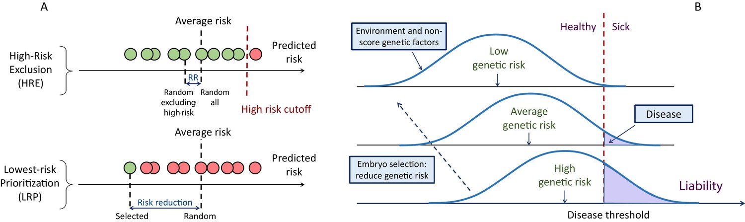
The first strategy we consider is aimed only at avoiding high-risk embryos, consistent with studies of the potential clinical utility of PRSs in adults (Chatterjee et al., 2016; Dai et al., 2019; Gibson, 2019; Khera et al., 2018; Mars et al., 2020; Mavaddat et al., 2019; Torkamani et al., 2018). For example, the first case report presented on PES described the identification and exclusion of embryos with extremely high (top 2-percentiles) PRS (Treff et al., 2019a). We term this strategy ‘high-risk exclusion’ (HRE: Figure 1A, upper panel). Under HRE, after high-risk embryos are set aside, an embryo is randomly selected for implantation among the remaining available embryos. (In the case that all embryos are high-risk, we assume a random embryo is selected among them.)

Figure 1

Download asset Open asset

A schematic of the liability threshold model and polygenic embryo screening.

(A) An illustration of the embryo selection strategies considered in this report. In the figure, each embryo is shown as a filled circle, and embryos are sorted based on their predicted risk, that is, their polygenic risk scores. Excluded embryos are shown in pink, and embryos that can be implanted in green. The risk reduction (RR) is indicated as the difference in risk between a randomly selected embryo (if no polygenic scoring was performed) and the embryo selected based on one of two strategies. In *high-risk exclusion* (HRE), the embryo selected for implantation is random, as long as its PRS is under a high-risk cutoff (usually the top few PRS percentiles). If all embryos are high-risk, a random embryo is selected. In *lowest-risk prioritization* (LRP), the embryo with the lowest PRS is selected for implantation. As we describe below, the LRP strategy yields much larger disease risk reductions. (B) An illustration of the liability threshold model (LTM). Under the LTM, each disease has an underlying (unobserved) liability, and an individual is affected if the total liability is above a threshold. The liability is composed of a genetic component and an environmental component, both assumed to be normally distributed in the population. For a given genetic risk (represented here by the polygenic risk score), the liability is the sum of that risk, plus a normally distributed *residual* component (environmental + genetic factors not captured by the PRS). For an individual with high genetic risk (bottom curve), even a modestly elevated (and thus, commonly-occurring) liability-increasing environment will lead to disease. For an individual with low genetic risk (top curve), only an extreme environment will push the liability beyond the disease threshold. Thus, disease risk reduction can be achieved with embryo screening by lowering the genetic risk of the implanted embryo. (Note that for the purpose of illustration, panel (B) displays three discrete levels of genetic risk, although in reality, the PRS is continuously distributed).

An alternative selection strategy is to use the embryo with the lowest PRS. Ranking and prioritizing embryos for implantation based on morphology is common in current IVF practice (Bormann et al., 2020; Montag et al., 2013; Rhenman et al., 2015). If ranking is instead based on a disease PRS, the embryo with the lowest PRS could be selected, without any recourse to high-risk PRS thresholds. Such an approach was suggested by another recent publication from the same company (based on a multi-disease index), but outcomes were only examined in the context of sibling pairs (Treff et al., 2020). We term the implantation of the embryo with the lowest PRS as ‘lowest-risk-prioritization’ (LRP; Figure 1A, lower panel).

In the following, we describe the theoretical risk reduction that can be achieved under these selection strategies. Our statistical approach is based on the liability threshold model (LTM; Falconer, 1967). The LTM represents disease risk as a continuous liability, comprising genetic and environmental risk factors, under the assumption that individuals with liability exceeding a threshold are affected. The liability threshold model has been shown to be consistent with data from family-based transmission studies (Wray and Goddard, 2010) and GWAS data (Visscher and Wray, 2015). Consequently, we define the disease risk of a given embryo probabilistically, as the chance that, given its PRS, its liability will cross the threshold at any point after birth (Figure 1B).

We use the following notation. We define the predictive power of a PRS as the proportion of variance in the liability of the disease explained by the score (Dudbridge, 2013), and denote it as $r_{p s}^{2}$ . We quantify the outcome of PES in two ways: the relative risk reduction (RRR) is defined as $RRR = \frac{K - P (disease)}{K} = 1 - \frac{P (disease)}{K}$ , where $K$ is the disease prevalence and $P (d i s e a s e)$ is the probability of the selected embryo to be affected; the absolute risk reduction (ARR) is defined as $K - P (d i s e a s e)$ . For example, if a disease has prevalence of 5% and the selected embryo has a probability of 3% to be affected, the RRR is 40%, and the ARR is 2% points. We computed the RRR and ARR analytically under each selection strategy, and for various values for the disease prevalence, the strength of the PRS, embryo exclusion thresholds, and other parameters. The mathematical basis of the calculations is summarized in Materials and methods, and detailed in the Appendix.

The risk reduction under the high-risk exclusion strategy

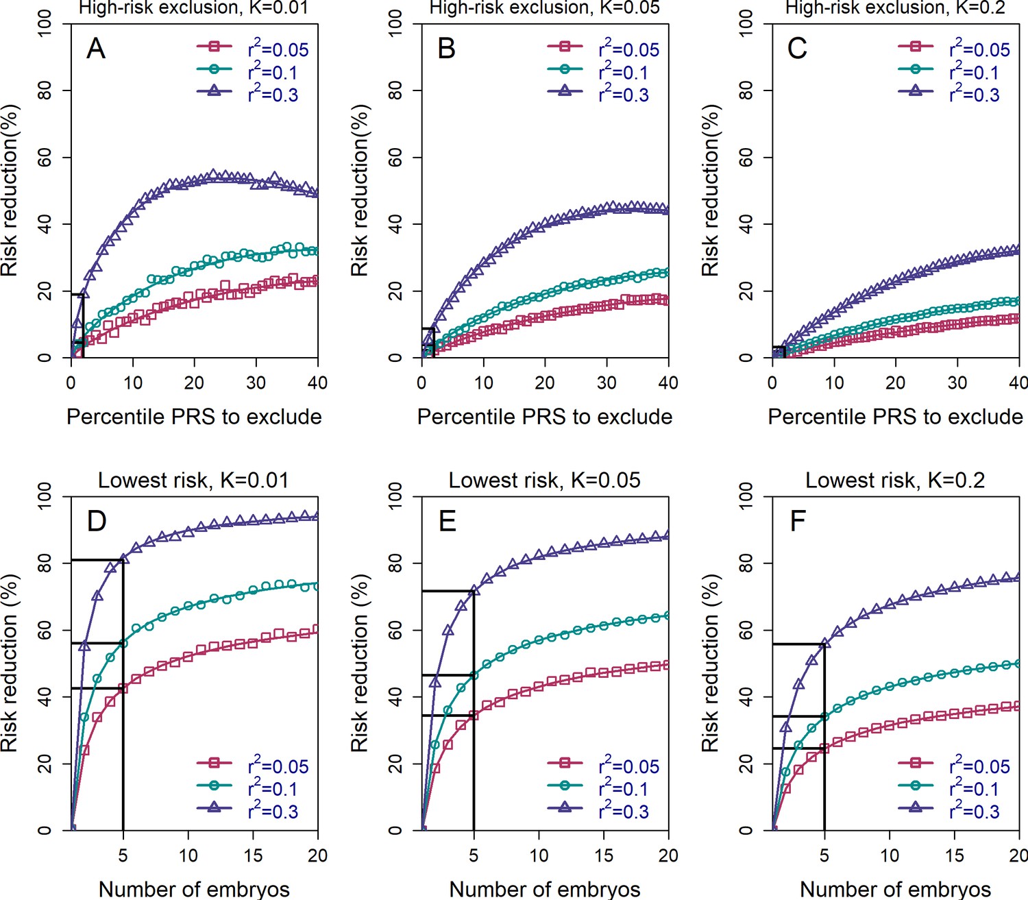
In Figure 2 (upper row), we show the relative risk reduction achievable under the HRE strategy with $n = 5$ embryos. Under the 2-percentile threshold (straight black lines), the reduction in risk is limited: the RRR is <10% in all scenarios where $r_{p s}^{2} \leq 0.1$ . Currently, $r_{p s}^{2} \approx 0.1$ (on the liability scale) is the upper limit of the predictive power of PRSs for most complex diseases (Lambert et al., 2021), with the exception of a few disorders with large-effect common variants (such as Alzheimer’s disease or type 1 diabetes) (Sharp et al., 2019; Zhang et al., 2020). In the future, more accurate PRSs are expected. However, the common-variant SNP heritability is at most ≈30% even for the most heritable diseases such as schizophrenia and celiac disease (Holland et al., 2020; Zhang et al., 2018), and it was recently suggested that $r_{p s}^{2} = 0.3$ is the maximal realistic value for the foreseeable future (Wray et al., 2021). At this value, relative risk reduction would be 20% for $K = 0.01$ , 9% for $K = 0.05$ , and 3% for $K = 0.2$ . These gains achieved with HRE are small because the overwhelming majority of affected individuals do not have extreme scores (Murray et al., 2021; Wald and Old, 2019).

Figure 2 with 3 supplements see all

Download asset Open asset

The relative risk reduction across selection strategies and disease parameters.

The relative risk reduction (RRR) is defined as $(K - P (disease)) / K$ , where $K$ is the disease prevalence, and $P (disease)$ is the probability of the implanted embryo to become affected. The RRR is shown for the high-risk exclusion (HRE) strategy in the upper row (panels (A–C)), and for the lowest-risk prioritization (LRP) in the lower row (panels (D–F)). See Figure 1 for the definitions of the strategies. Results are shown for values of $K = 0.01, 0.05$ and $0.2$ (panels (A–C), respectively), and within each panel, for variance explained by the PRS (on the liability scale) $r_{p s}^{2} = 0.05, 0.1$ , and $0.3$ (legends). Symbols denote the results of Monte-Carlo simulations (Materials and methods), where PRSs of embryos were drawn based on a multivariate normal distribution, assuming PRSs are standardized to have zero mean and variance $r_{p s}^{2}$ , and accounting for the genetic similarity between siblings (Equation 4 in the Appendix). In each simulated set of $n$ sibling embryos ( $n = 5$ for all simulations under HRE), one embryo was selected according to the selection strategy. The liability of the selected embryo was computed by adding a residual component (drawn from a normal distribution with zero mean and variance $1 - r_{p s}^{2}$ ) to its polygenic score. The embryo was considered affected if its liability exceeded $z_{K}$ , the (upper) $K$ -quantile of the standard normal distribution. We repeated the simulations over 10⁶ sets of embryos and computed the disease risk. In each panel, curves correspond to theory: Equation (31) in the Appendix for the HRE strategy, and Equation (20) in the Appendix for the LRP strategy. Black straight lines correspond to the RRR achieved when excluding embryos at the top 2% of the PRS (for HRE, upper panels) or for selecting the lowest risk embryo out of $n = 5$ (for LRP, lower panels).

Risk reduction increases as the threshold for exclusion is expanded to include the top quartile of scores, and then reaches a maximum at ≈25-50% under a range of prevalence and $r_{p s}^{2}$ values. For all these simulations, we set the number of available (testable) embryos to $n = 5$ (Dahdouh, 2021; Sunkara et al., 2011), although we acknowledge that the number of viable embryos may be much lower for many couples seeking IVF services for infertility (Smith et al., 2015). Simulations show that these estimates do not change much with increasing the number of embryos (see Figure 2—figure supplement 1). This holds especially at more extreme threshold values, since most batches of $n$ embryos will not contain any embryos with a PRS within, for example, the top 2-percentiles.

It should be noted that the relative risk reduction does not increase monotonically under HRE. Under our definition, whenever all embryos are high risk, an embryo is selected at random. Thus, at the extreme case when all embryos (i.e. top 100%) are designated as high risk, an embryo is selected at random at all times, and the relative risk reduction reduces to zero. We chose this definition of the HRE strategy because it does not involve ranking of the embryos. However, we can also consider an alternative strategy: if all embryos are high risk, the embryo with the lowest PRS is selected. Here, the RRR is expected to increase when increasing the threshold and designating more embryos as high risk, which we confirm in Figure 2—figure supplement 2. When the threshold is at 100% (all embryos are high risk), this alternative strategy (which we do not further consider) reduces to the lowest-risk prioritization strategy, which we study next.

The risk reduction under the lowest-risk prioritization strategy

The HRE strategy treats all non-high-risk embryos equally. In practice, we expect most, or even all, embryos to be designated as non-high-risk, given the recent focus on the top PRS percentiles in the literature (e.g. Khera et al., 2018). However, as we have seen, this strategy leads to very little risk reduction. In Figure 2 (lower panels), we show the expected RRR for the lowest-risk prioritization strategy, under which we prioritize for implantation the embryo with the lowest PRS, regardless of any PRS cutoff. Indeed, under the LRP strategy, risk reductions are substantially greater than in HRE. For example, with $n = 5$ available embryos, RRR>20% across the entire range of prevalence and $r_{p s}^{2}$ parameters considered, and can reach ≈50% for $K \leq 5 %$ and $r_{p s}^{2} = 0.1$ , and even ≈80% for $K = 1 %$ and $r_{p s}^{2} = 0.3$ . While RRR continues to increase as the number of available embryos increases, the gains are quickly diminishing after $n = 5$ . On the other hand, Figure 2 also demonstrates that RRR drops steeply if the number of embryos falls below $n = 5$ , although the lower bound for RRR when just two embryos are available (≈20% for many scenarios) is still comparable to the upper bound of the HRE strategy for a greater number of embryos.

Effects of PES on dichotomous vs quantitative traits

Our results demonstrate that, contrary to our previous study reporting only small effects of PES for quantitative traits (Karavani et al., 2019), PES can generate substantial relative risk reductions for diseases under the LRP strategy. To understand the relation between continuous and binary traits, consider an example involving IQ. Our estimate for the mean gain in IQ that could be achieved by selecting the embryo with the highest IQ polygenic score is approximately ≈2.5 IQ points (Karavani et al., 2019). Now assume that individuals with IQ<70 (2 SDs below the mean) are considered 'affected' according to a dichotomized trait of 'cognitive impairment'. Among individuals with IQ<70, the proportion of individuals with IQ in the range [67.5,70] is 33.5% (assuming a normal distribution). A gain of 2.5 points would shift such offspring beyond the threshold for 'cognitive impairment', resulting in a corresponding 33.5% reduction in risk of being 'affected'. (Note that the above explanation is intended to provide an intuition and ignores any variability in the gain.) Figure 2—figure supplement 3 utilizes statistical modeling (with $r_{p s}^{2}$ derived from recent GWAS for intelligence [Savage et al., 2018]) to demonstrate that substantial risk reductions can be achieved for a dichotomized trait, including when selecting out of just three embryos (panel (A)). Panel (B) extends these results to data for LDL cholesterol (with $r_{p s}^{2}$ derived from Weissbrod et al., 2021); given $n = 5$ embryos and the currently available PRS for LDL-C levels, risk reductions for 'high cholesterol' range from 40 to 60%, depending on the LDL level used to define the categorical trait. Thus, while implanting the embryo with the most favorable PRS is expected to result in very modest gains in an underlying quantitative trait, it is at the same time effective in avoiding embryos at the unfavorable tail of the trait.

Effects of parental PRS and disease status

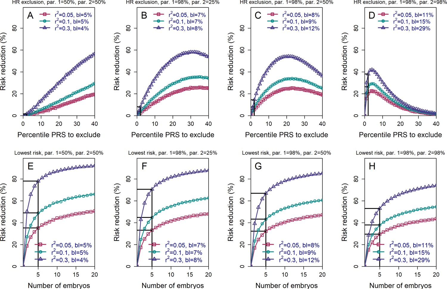
We next examined the effects of parental PRSs on the achievable risk reduction (Materials and methods, see also the Appendix), given that families with high genetic risk for a given disease may be more likely to seek PES. Figure 3 demonstrates that, as expected, the HRE strategy shows greater relative risk reduction as parental PRS increases, in particular when excluding only very high-scoring embryos. This result follows directly from the fact that, on average, offspring will tend to have PRS scores near the mid-parental PRS value. In contrast, the relative RR (although not the absolute RR; see next section) for the LRP strategy somewhat declines as parental PRSs increase. Nevertheless, the RRR for the LRP strategy remains greater than that for the HRE strategy across all parameters (as expected by the definitions of these strategies).

Figure 3 with 2 supplements see all

Download asset Open asset

The relative risk reduction when the polygenic risk scores of the parents are known.

Panels (A)-(D) are for the *high-risk exclusion* (HRE) strategy, while panels (E)-(H) are for the *lowest-risk prioritization* (LRP) strategy. All details are as in Figure 2, except the following. First, we fixed the prevalence to $K = 5 %$ . Second, in the simulations, we drew the PRS of each embryo as $s_{i} = x_{i} + c$ ( $i = 1, \dots, n$ ), where $x_{i}$ is an embryo-specific component (independent across embryos) and $c$ is the shared component, also representing the mean parental PRS (Materials and methods). This is so far as in Figure 2; however, here we assumed that $c$ is given, equal to the average PRSs of the two parents. In each panel, we consider a different pair of PRSs for the parents. For example, in panels (A) and (E), both parents ('par. 1' and 'par. 2') have PRS equal to the 50% percentile of the PRS distribution; in panels (B) and (F), one parent has PRS equal to the 98% percentile of the PRS distribution, while the other has PRS equal to the 25% percentile; and so on. Third, in the simulations, we computed the risk reduction (according to either strategy) relative to a baseline, obtained from the same sets of simulations, when we always selected the first embryo. The baseline risk is indicated in each legend as 'bl'. Note that the baseline risk depends on the variance explained by the PRS, because the parental PRSs are determined as percentiles of the population distribution of the score, which has variance $r_{p s}^{2}$ . Finally, we computed the theoretical disease risk for the HRE strategy using Equation (29) from the Appendix, the disease risk for the LRP strategy using Equation (23), and the relative risk reduction (shown in curves) for both strategies using Equation (36).

It is also conceivable that families may be more likely to seek PES when one or both prospective parents is affected by a given disease. In Figure 3—figure supplement 1, we plot the RRR under the HRE and LRP strategies given that the parents are both healthy, both affected, or one of each (where we fixed the prevalence $K = 5 %$ and the heritability to $h^{2} = 40 %$ ). The figure illustrates that parental disease status has relatively little impact on the expected RRR (especially in comparison to the changes under HRE when conditioning on the actual parental PRSs). This is because, as long as $r_{p s}^{2} ≪ 1,$ parental disease does not necessarily provide much information about parental PRS, and thus does not strongly constrain the number of risk alleles available to each embryo.

Absolute vs relative risk

The above results were presented in terms of relative risk reductions. However, Figure 3—figure supplement 1 also shows the baseline risk of an embryo of parents with a given disease status. For example, when one of the parents is affected, selecting the lowest risk embryo out of $n = 5$ (for a realistic $r_{p s}^{2} = 0.1$ ) reduces the risk from 10.0% to only 5.8%, thus nearly restoring the risk of the future child to the population prevalence (5%). More generally, we plot the absolute risk reduction (ARR) under the HRE and LRP strategies in Figure 3—figure supplement 2 for a few values of the parental PRSs. Notably, while RRRs under the LRP strategy somewhat decrease with increasing parental PRSs, the ARRs substantially increase, in accordance with an expectation that PES in higher risk parents should eliminate more disease cases.

The clinical interpretation of these absolute risk changes will vary based on the population prevalence of the disorder (or the baseline risk of specific parents), and can offer a very different perspective on the magnitude of the effects (Gordis, 2014; Lázaro-Muñoz et al., 2021; Murray et al., 2021). In particular, for a rare disease, large relative risk reductions may result in very small changes in absolute risk. As an example, schizophrenia is a highly heritable (Sullivan et al., 2003) serious mental illness with prevalence of at most 1% (Perälä et al., 2007). The most recent large-scale GWAS meta-analysis for schizophrenia (Ripke et al., 2020) has reported that a PRS accounts for approximately 8% of the variance on the liability scale. Our model shows that a 52% RRR is attainable using the LRP strategy with $n = 5$ embryos. However, this translates to only ≈0.5 percentage points reduction on the absolute scale: a randomly-selected embryo would have a 99% chance of not developing schizophrenia, compared to a 99.5% chance for an embryo selected according to LRP. In the case of a more common disease such as type 2 diabetes, with a lifetime prevalence in excess of 20% in the United States (Geiss et al., 2014), the RRR with $n = 5$ embryos (if the full SNP heritability of 17% [Zhang et al., 2018] were achieved) is 43%, which would correspond to >8 percentage points reduction in absolute risk.

Variability of the risk reduction across couples

The results depicted in Figure 2 describe the average risk reduction across the population, whereas the results in Figure 3 demonstrate results for specific combinations of parental risk scores. However, it remains unclear whether the large average risk reductions observed under the LRP strategy are driven by only a small proportion of couples. More generally, we would like to fully characterize the dependence of the risk reduction on parental PRSs, which could be of interest to physicians and couples in real-world settings.

To address these questions, we define a new risk reduction index, which we term the per-couple relative risk reduction, or pcRRR. Informally, the pcRRR is the relative risk reduction conditional of the PRSs of the couple. Mathematically, $pcRRR(couple) = 1 - \frac{P_{s} (disease| couple)}{P_{r} (disease| couple)}$ . Here, $P_{s} (disease | couple)$ is the probability that the (PRS-based) selected embryo is affected given the PRSs of the couple, and $P_{r} (disease | couple)$ is similarly defined for a randomly selected embryo. Conveniently, the pcRRR depends only on the average of the maternal and paternal PRSs, which we denote as $c$ . We calculated $pcRRR (c)$ analytically under the LRP strategy (the Appendix), as well as computed the distribution of $pcRRR (c)$ across all couples in the population.

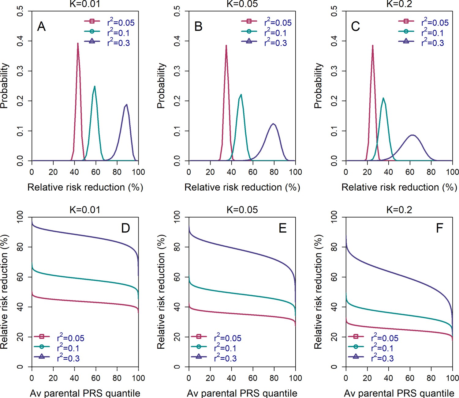
We show the distribution of $pcRRR (c)$ in Figure 4, panels (A)-(C). The results demonstrate that the pcRRR is relatively narrowly distributed around its mean, for all values of the prevalence ( $K$ ) considered. The distribution becomes somewhat wider (and left-tailed) for the most extreme $r_{p s}^{2}$ (0.3). Thus, the population-averaged RRRs are not driven by a small proportion of the couples. In agreement, the pcRRR depends only weakly on the average parental PRS, as can be seen in panels (D)-(F).

Figure 4

Download asset Open asset

The variability in the relative risk reduction across couples.

We considered only the *lowest-risk prioritization* strategy. In panels (A–C), we computed the theoretical distribution of the *per-couple* relative risk reduction, as explained in the Appendix Section 5. Briefly, the *per-couple* RRR is defined as $1 - P_{s} (disease | c) / P_{r} (disease | c)$ , where $P_{s} (disease| c)$ is the probability of an embryo selected based on its PRS to be affected and $P_{r} (disease | c)$ is the probability of a randomly selected embryo to be affected, both conditional on the given couple. Our modeling suggests that $c$ , which is the average of the paternal and maternal PRSs, is the only determinant of the relative risk reduction of a given couple. We computed the distribution of the *per-couple* RRR based on 10⁴ quantiles of $c$ , thus covering all hypothetical couples in the population. The number of embryos was set to $n = 5$ in all panels. Panels (A–C) correspond to prevalence of $K = 0.01, 0.05$ , and $0.02$ , respectively. In panels (D–F), we plot the theoretical RRR vs the quantile of the average parental PRS $c$ (see Appendix Section 5.1).

We note that the per-couple relative risk reduction is also an average, over all possible batches of $n$ embryos of the couple. One may thus ask what is the distribution of possible RRRs across these batches. We provide a short discussion in the Appendix (Section 5.3).

Pleiotropic effects of selection on genetically negatively correlated diseases

Polygenic risk scores are often correlated across diseases (Watanabe et al., 2019; Zheng et al., 2017). Therefore, selecting based on the PRS of one disease may increase or decrease risk for other diseases. While a full analysis of screening for multiple diseases is left for future work, our simulation framework allows us to investigate the potential harmful effects of prioritizing embryos for one disease, in case that disease is negatively correlated with another disease (see the Appendix). We considered genetic correlations between diseases taking the values $ρ = (- 0.05, - 0.1, - 0.15, - 0.2, - 0.3)$ . [The most negative correlation between two diseases reported in LDHub (https://ldsc.broadinstitute.org/ldhub/) is −0.3, occurring between ulcerative colitis and chronic kidney disease (Zheng et al., 2017).] In general, negative correlations between diseases are uncommon, and when they occur, typical correlations are about −0.1.

Figure 5 shows the simulated risk reduction for the target disease and the risk increase for the correlated disease, across different values of $ρ$ and for three values of the prevalence $K$ (panels (A)-(C); assumed equal for the two diseases), all under the LRP strategy. In all panels, we used $r_{p s}^{2} = 0.1$ for both diseases. The relative risk reduction for the target disease is, as expected, always higher in absolute value than the risk increase of the correlated disease. For typical values of $ρ = - 0.1$ and $n = 5$ , the relative increase in risk of the correlated disease is relatively small, at ≈6% for $K \leq 0.05$ and ≈3.5% for $K = 0.2$ . However, for strong negative correlation ( $ρ = - 0.3$ ) the increase in risk can reach 22%, 16%, or 11% for $K = 0.01, 0.05$ and $0.2$ , respectively. Thus, care must be taken in the unique setting when the target disease is strongly negatively correlated with another disease.

Figure 5

Download asset Open asset

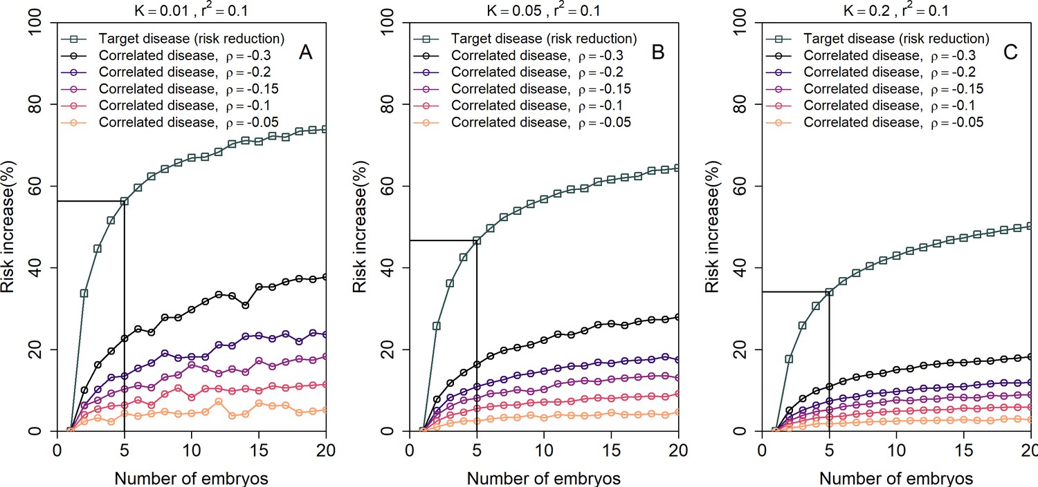
The increase in the risk of a negatively correlated disease due to polygenic embryo screening.

We simulated two diseases that have genetic correlation $ρ < 0$ . We assumed that the prevalence $K$ is equal between the two diseases ( $K = 0.01, 0.05$ and $0.2$ : panels (A)-(C), respectively), and that $r_{p s}^{2} = 0.1$ for both diseases. We simulated polygenic scores for the two diseases in $n$ embryos in each of 10⁶ couples. For each couple, we selected the embryo either randomly or based on having the lowest PRS for the target disease. We then computed the risk of the embryo to have each disease as in the main analyses, by drawing the residual component of the liability and designating the embryo as affected if the total liability exceeded a threshold. The relative risk reduction of the target disease is shown as gray squares (and connecting lines) at the top of each plot. The relative risk *increase* for the correlated disease is shown in colored circles (and connecting lines), with different colors corresponding to different values of $ρ$ (see legend). Note that the risk reduction for the target disease is independent of $ρ$ .

Simulations based on real genomes from case-control studies

Our analysis so far has been limited to mathematical analysis and simulations based on a statistical model. In principle, it would be desirable to compare our predictions to results based on real data. However, clearly, no real genomic and phenotypic data exist that would correspond to our setting, nor could such data be ethically or practically generated. Thus, we resort to a ‘hybrid’ approach, in which we simulate the genomes of embryos based on real genomic data from case-control studies. This approach is similar to the one we have previously used for studying polygenic embryo screening for traits (Karavani et al., 2019).

Briefly, our approach is as follows. We consider separately two diseases with somewhat differing genetic architecture: schizophrenia, which is amongst the most polygenic complex diseases, with no common loci of high effect size, and Crohn’s disease, which is estimated to be less polygenic, and has several common loci with much larger effects than those found in schizophrenia (O'Connor et al., 2019). For each disease, we used genomes of unrelated individuals drawn from case-control studies. For schizophrenia, we used ≈900 cases and ≈1600 controls of Ashkenazi Jewish ancestry, while for Crohn’s, we used ≈150 cases and ≈100 controls of European ancestry. We then generated 'virtual couples' by randomly mating pairs of individuals, regardless of sex. For each couple, we simulate the genomes of $n$ hypothetical embryos, based on the laws of Mendelian inheritance and by randomly placing crossovers according to genetic map distances. In parallel, we used the 'parental' genomes to learn a logistic regression model that predicts the disease risk given a PRS computed based on existing summary statistics. We then computed the PRS of each simulated embryo, and predicted the risk that embryo to be affected. Finally, we compared the risk of disease between a population in which one embryo per couple is selected at random, vs. a population in which one embryo is selected based on its PRS. For complete details, see Materials and methods.

In Figure 6, we plot the results for the relative risk reduction for schizophrenia (panels (A) and (B)) and Crohn’s disease (panels (C) and (D)). For each disease, we consider both the HRE and LRP strategies. The analytical predictions closely match the empirical risk reductions generated in the simulations, except for a slight overestimation of the RRR under the LRP strategy. Nevertheless, for both schizophrenia and Crohn’s disease, we empirically observe that RRRs as high as ≈45% are achievable with $n = 5$ embryos. In contrast, under the HRE strategy and when excluding embryos at the top 2% risk percentiles, risk reductions are very small, in agreement with the theoretical predictions. These results thus provide support to the robustness of our statistical model.

Figure 6 with 1 supplement see all

Download asset Open asset

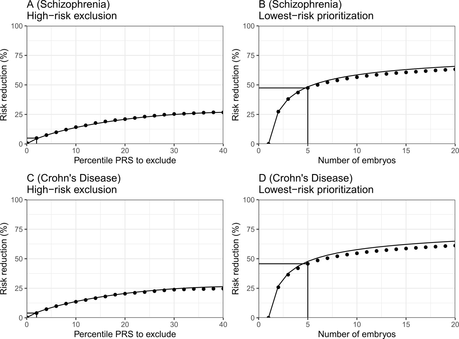
The empirical relative risk reduction in simulated embryos based on genomes from case-control studies of schizophrenia and Crohn’s disease.

We used ≈900 cases and ≈1600 controls for schizophrenia, and ≈150 cases and ≈100 controls for Crohn’s. For each disease, we drew 5000 random 'virtual couples', regardless of sex, but correcting for case/control ascertainment. For each such random couple, we simulated the genomes of up to $n = 20$ embryos (children) based on Mendelian segregation and published recombination maps. For each embryo, we computed the PRS for the given disease (schizophrenia or Crohn’s) using the most recent summary statistics that exclude our cohort. We computed the risk of each embryo to be affected based on a logistic regression model we learned in the 'parental' cohort. Panels (A) and (B) show results for schizophrenia, while panels (C) and (D) show results for Crohn’s. In panels (A) and (C), we plot the relative risk reduction (RRR) under the *high-risk exclusion* (HRE) selection strategy, in which an embryo was randomly selected (out of $n = 5$ embryos), unless its PRS was above a given percentile. The RRR was computed against a baseline strategy of selection of an embryo at random and is plotted vs the exclusion percentile. In panels (B) and (D), we show the relative risk reduction under the *lowest-risk prioritization* (LRP) strategy, in which the embryo with the lowest PRS was selected. We plot the RRR vs the number of embryos $n$ . In all panels, dots correspond to the results of simulations, and solid lines correspond to the theory. The theory was computed assuming prevalence of 1% for schizophrenia and 0.5% for Crohn’s, and variance explained on the liability scale of $r_{p s}^{2} = 0.068$ for schizophrenia $r_{p s}^{2} = 0.056$ for Crohn’s (calculated using the method of Lee et al., 2012). Further details are provided in Materials and methods.

To further investigate the assumptions of our model, we test in Figure 6—figure supplement 1 two intermediate predictions. The first is that the variance of the PRSs of embryos of a given couple should not depend on the average parental PRS. This is indeed the case (panels (A) and (C)), with the only exception of an uptick of the variance at very low parental PRSs for schizophrenia. The second prediction is that the variance across embryos is half of the variance in the parental population. The empirical results again show reasonable agreement with the theoretical prediction (panels (B) and (D)). The empirical variance (averaged across couples) was slightly lower than expected (by ≈4% for schizophrenia and ≈14% for Crohn’s), which may explain our slight overestimation of the expected RRR under the LRP strategy.

Discussion

In this paper, we used statistical modeling to evaluate the expected outcomes of screening embryos based on polygenic risk scores for a single disease. We predicted the relative and absolute risk reductions, either at the population level or at the level of individual couples. Our model is flexible, allowing us to provide predictions across various values of, for example, the PRS strength, the disease prevalence, the parental PRS or disease status, and the number of available embryos. We presented a comprehensive analysis of the expected outcomes across various settings, including when there is a concern about a second disease negatively correlated with the target disease. We finally validated our modeling assumptions using genomes from case-control studies. Our publicly available code could help researchers and other stakeholders estimate the expected outcomes for settings we did not cover.

Our most notable result was that a crucial determinant of risk reduction is the selection strategy. The use of PRS in adults has focused on those at highest risk (Chatterjee et al., 2016; Dai et al., 2019; Gibson, 2019; Khera et al., 2018; Mars et al., 2020; Mavaddat et al., 2019; Torkamani et al., 2018), for whom there may be maximal clinical benefit of screening and intervention. However, as PRSs have relatively low sensitivity, such a strategy is relatively ineffective in reducing the overall population disease burden (Ala-Korpela and Holmes, 2020; Wald and Old, 2019). Similarly, in the context of PES, exclusion of high-risk embryos will result in relatively modest risk reductions. By contrast, selecting the embryo with the lowest PRS may result in large reductions in relative risk.

While our prior work (Karavani et al., 2019) demonstrated that PES would have a small effect on quantitative traits, here we show that a small reduction in the liability can lead to a large reduction in the proportion of affected individuals. This is fundamentally a property of a threshold character with an underlying normally distributed continuous liability. For such traits, most of the individuals in the extreme of the liability distribution (i.e. the ones affected) are concentrated very near the threshold. Thus, even slightly reducing their liability can move a large proportion of affected individuals below the disease threshold. However, it should be noted that conventional thresholds for defining presence of disease may contain some degree of arbitrariness if the underlying distribution of pathophysiology is truly continuous. Consequently, the effects on ultimate morbidity may depend on the validity of the threshold itself (Davidson and Kahn, 2016).

We investigated how the range of potential PES outcomes varies with the PRSs of the parents or with their disease status. Under the HRE strategy, if only excluding embryos at the few topmost risk percentiles, the RRR is very small when the parents have low PRSs, and vice versa (Figure 3, panels (A)-(D)). This is expected, as excluding high PRS embryos will be effective only for couples who are likely to have many such embryos. Under the LRP strategy, the RRR depends only weakly on the parental PRSs (Figure 3, panels (E)-(H), and Figure 4). Under both strategies, the relative risk reduction depends only weakly on the parental disease status, as parental disease status is a weak signal for the underlying PRS. However, the absolute risk reduction increases substantially with increasing parental PRSs (Figure 3—figure supplement 2) and when one or more parents are affected.

Our study has several limitations. First, our results assume an infinitesimal genetic architecture for the disease, which may not be appropriate for oligogenic diseases and is not relevant for monogenic disorders. However, it has been repeatedly demonstrated that common, complex traits and diseases are highly polygenic (Gazal et al., 2017; Holland et al., 2020; O'Connor et al., 2019; Shi et al., 2016; Zeng et al., 2018; Zeng et al., 2021). For example, it was recently estimated that for almost all traits and diseases examined, the number of independently associated loci was at least ≈350, reaching ≈10,000 or more for cognitive and psychiatric phenotypes (O'Connor et al., 2019). This provides more than sufficient variability for the PRS to attain a normal distribution in the population and for our modeling assumptions to hold. Indeed, our empirical results for schizophrenia and Crohn’s disease, two diseases with somewhat different genetic architectures, agreed reasonably well with the theoretical predictions. However, our models would need to be substantially adjusted in the presence of variants of very large effect, such as inherited or de novo coding variants or copy number variants, for example, as in autism (Satterstrom et al., 2020; Takumi and Tamada, 2018).

Additionally, our model relies on several simplifying statistical assumptions. For example, we did not explicitly model assortative mating, although this seems reasonable given that for genetic disease risk, correlation between parents is weak (Rawlik et al., 2019), and given that our previous study of traits showed no difference in the results between real and random couples (Karavani et al., 2019). This deficiency is also partly ameliorated by our modeling of the risk reduction when explicitly given the parental PRSs or disease status. Another assumption we made is that environmental influences on the child’s phenotype are independent of those that have influenced the parents (when conditioning on the parental disease status). However, this is reasonable given that family-specific environmental effect have been shown to be weak for complex diseases (Wang et al., 2017). For a discussion of additional model assumptions, see Appendix section 10.

Perhaps more importantly, we assumed throughout that $r_{p s}^{2}$ represents the realistic accuracy of the PRS achievable, within-family, in a real-world setting in the target population. However, the realistically achievable $r_{p s}^{2}$ may be lower than reported in the original publications that have generated the scores. For example, the accuracy of PRSs is sub-optimal when applied in non-European populations and across different socio-economic groups (Duncan et al., 2019; Mostafavi et al., 2020). A PRS that was tested on adults may be less accurate in the next generation. Additionally, the variance explained by the score, as estimated in samples of unrelated individuals, is inflated due to population stratification, assortative mating, and indirect parental effects (Kong et al., 2018; Young et al., 2019; Morris et al., 2020; Mostafavi et al., 2020). The latter, also called 'genetic nurture', refers to trait-modifying environmental effects induced by the parents based on their genotypes. These effects do not contribute to prediction accuracy when comparing polygenic scores between siblings (as when screening IVF embryos), and thus, the variance explained by polygenic scores in this setting can be substantially reduced, in particular for cognitive and behavioral traits (Howe et al., 2021; Selzam et al., 2019). Our risk reduction estimates thus represent an upper bound relative to real-world scenarios. On the other hand, recent empirical work on within-family disease risk prediction showed that the reduction in accuracy is at most modest (Lello et al., 2020), and within-siblings-GWAS yielded similar results to unrelated-GWAS for most physiological traits (Howe et al., 2021). Additionally, accuracy in non-European populations is rapidly improving due to the establishment of national biobanks in non-European countries (Koyama et al., 2020; Vujkovic et al., 2020) and improvement in methods for transferring scores into non-European populations (Amariuta et al., 2020; Cai et al., 2021). Either way, the analytical results presented in this paper are formulated generally as a function of the achievable accuracy $r_{p s}^{2}$ , and as such, users can substitute values relevant to their specific target population and disease.

Another major limitation of this work is that we have only considered screening for a single disease. In reality, couples may seek to profile an embryo on the basis of multiple disease PRSs simultaneously, or based a global measure of lifespan or healthspan (Sakaue et al., 2020; Timmers et al., 2020; Zenin et al., 2019). This is likely to reduce the per-disease risk reduction, as we have previously observed for quantitative traits (Karavani et al., 2019), but will also likely be more cost effective (Treff et al., 2020; Gwern, 2018). PES for multiple diseases requires the formulation and analysis of new selection strategies and is substantially more mathematically complex; we therefore leave it for future studies.

As our approach was statistical in nature, it is important to place our results in the context of real-world clinical practice of assisted reproductive technology. The number of embryos utilized in the calculations in the present study refers to viable embryos that could lead to live birth, which can be substantially smaller than the raw number of fertilized oocytes or even the number of implantable embryos at day 5. This consideration is especially important given the steep drop in risk reduction when the number of available embryos drops below 5 (Figure 2). In fact, many IVF cycles do not achieve any live birth. Rates of live birth decline with maternal age, in particular after age 40 (Smith et al., 2015); for women of age >42, fewer than 4% of IVF cycles result in live births, making PES impractical. On the other hand, success rates will likely be higher for young prospective parents who seek PES to reduce disease risk but do not suffer from infertility. However, the prospect of elective IVF for the purpose of PES in such couples must be weighed against the potential risks of these invasive procedures to the mother and child (Dayan et al., 2019; Luke, 2017).

A different concern is whether the embryo biopsy (which is required for genotyping) may cause risk to the viability and future health of the embryo. Several recent studies have demonstrated no evidence for potential adverse effects of trophectoderm biopsy on rates of successful implantation, fetal anomalies, and live birth (Awadalla et al., 2021; He et al., 2019; Riestenberg et al., 2021; Tiegs et al., 2021). Moreover, no significant adverse effects have been detected for postnatal child development in a recent meta-analysis (Natsuaki and Dimler, 2018). On the other hand, a number of studies have reported that trophectoderm biopsy was associated with pregnancy complications, including preterm birth, pre-eclampsia, and hypertensive disorders of pregnancy (Li et al., 2021; Zhang et al., 2019; Makhijani et al., 2021). Specific variations in biopsy protocols may account for differences in outcomes across studies (Rubino et al., 2020). Newly developed techniques may allow in the future to genotype an embryo non-invasively based on DNA present in spent culture medium, although the accuracy of these methods is still being debated (Leaver and Wells, 2020). It should also be noted that, throughout this manuscript, we assumed the use of single embryo transfer.

Finally, the results of our study invite a debate regarding ethical and social implications. For example, the differential performance of PES across selection strategies and risk reduction metrics may be difficult to communicate to couples seeking assisted reproductive technologies (Cunningham et al., 2015; Wilkinson et al., 2019). Indeed, in the first PES case report, the couple elected to forego any implantation despite the availability of embryos that were designated as normal risk (Treff et al., 2019a). These difficulties are expected to exacerbate the already profound ethical issues raised by PES (as we have recently reviewed [Lázaro-Muñoz et al., 2021]), which include stigmatization (McCabe and McCabe, 2011), autonomy (including ‘choice overload’ [Hadar and Sood, 2014]), and equity (Sueoka, 2016). In addition, the ever-present specter of eugenics (Lombardo, 2018) may be especially salient in the context of the LRP strategy. How to juxtapose these difficulties with the potential public health benefits of PES is an open question. We thus call for urgent deliberations amongst key stakeholders (including researchers, clinicians, and patients) to address governance of PES and for the development of policy statements by professional societies. We hope that our statistical framework can provide an empirical foundation for these critical ethical and policy deliberations.

Materials and methods

Summary of the modeling results

Request a detailed protocol

In this section, we provide a brief overview of our model and derivations, with complete details appearing in the Appendix.

Our model is follows. We write the polygenic risk scores of a batch of $n$ IVF embryos as $(s_{1}, \dots, s_{n})$ , and generate the scores as $s_{i} = x_{i} + c$ . The $(x_{1}, \dots, x_{n})$ are embryo-specific independent random variables with distribution $x_{i} \sim N (0, r_{p s}^{2} / 2)$ , $r_{p s}^{2}$ is the proportion of variance in liability explained by the score, and $c$ is a shared component with distribution $c \sim N (0, r_{p s}^{2} / 2)$ , also representing the average of the maternal and paternal scores.

In each batch, an embryo is selected according to the selection strategy. Under high-risk exclusion, we select a random embryo with score $s < z_{q} r_{p s}$ , where $z_{q}$ is the $(1 - q)$ -quantile of the standard normal distribution. If no such embryo exists, we select a random embryo, but we also studied the strategy when in such a case, the lowest scoring embryo is selected. Under lowest-risk prioritization, we select the embryo with the lowest value of $s$ . We computed the liability of the selected embryo as $y = s + e$ , where $e \sim N (0, 1 - r_{p s}^{2})$ . We designate the embryo as affected if $y > z_{K}$ , where $z_{K}$ is the $(1 - K)$ -quantile of the standard normal distribution and $K$ is the disease prevalence. In the simulations, we computed the disease probability (for each parameter setting) as the fraction of batches (out of 10⁶ repeats) in which the selected embryo was affected. We also simulated the score and disease status of a second disease, which is not used for selecting the embryo, but may be negatively correlated with the target disease.

We computed the disease probability analytically using the following approaches. We first computed the distribution of the score of the selected embryo. For lowest-risk prioritization, we used the theory of order statistics. For high-risk exclusion, we first conditioned on the shared component $c$ , and then studied separately the case when all embryos are high-risk (i.e. have score $s > z_{q} r_{p s}$ ), in which the distribution of the unique component of the selected embryo ( $x$ ) is a normal variable truncated from below at $z_{q} r_{p s} - c$ , and the case when at least one embryo has score $s < z_{q} r_{p s}$ , in which $x$ is a normal variable truncated from above. We then integrated over the non-score liability components (and over $c$ in some of the settings) in order to obtain the probability of being affected. We solved the integrals in the final expressions numerically in R.

We computed the risk reduction based on the ratio between the risk of a child of a random couple when the embryo was selected by PRS and the population prevalence. We also provide explicit results for the case when the average parental PRS $c$ is known. These expressions allowed us to compute the distribution of risk reductions per-couple. Finally, when conditioning on the parental disease status, we integrated the disease probability of the selected embryo over the posterior distribution of the parental score and non-score genetic components. For full details and for an additional discussion of previous work and limitations, see the Appendix. R code is available at: https://github.com/scarmi/embryo_selection (copy archived at swh:1:rev:4cdc572582deb9b745e6844d96e0344914f4595e, Carmi, 2021) and https://github.com/dbackenroth/embryo_selection (copy archived at swh:1:rev:c65bf082fcb28434c271260560c4a4450dad76a3,; Backenroth, 2021).

Simulations based on genomes from case-control studies

Our main analysis has been limited to mathematical modeling of polygenic scores and their relation to disease risk. For obvious ethical and practical reasons, we could not validate our modeling predictions with actual experiments. Nevertheless, we could perform realistic simulations based on genomes from case-control studies, similarly to our previous work (Karavani et al., 2019). Our approach is as follows. We consider, separately, two diseases: schizophrenia and Crohn’s. For schizophrenia, we use ≈900 cases and ≈1600 controls of Ashkenazi Jewish ancestry, while for Crohn’s, we use ≈150 cases and ≈100 controls from the New York area. For each disease, we use these individuals, who are unrelated, to generate 'virtual couples' by randomly mating pairs of individuals. For each such 'couple', we simulate the genomes of $n$ hypothetical embryos, based on the laws of Mendelian inheritance and by randomly placing crossovers according to genetic map distances. In parallel, we use the same genomes to derive a logistic regression model that predicts the risk of disease given a PRS computed from the most recently available summary statistics (based on datasets not including the samples in our test cohorts). We then compute the PRS of each simulated embryo, and predict the risk of disease of that embryo. We finally compare the risk of disease between one randomly selected embryo per couple vs one embryo selected based on PRS. In the paragraphs below, we provide additional details.

The Ashkenazi schizophrenia cohort

Request a detailed protocol

The samples and the genotyping process were previously described (Lencz et al., 2013). Patients were recruited from hospitalized inpatients at seven medical centres in Israel and were diagnosed with schizophrenia or schizoaffective disorder. Samples from healthy Ashkenazi individuals were collected from volunteers at the Israeli Blood Bank. All subjects provided written informed consent, and corresponding institutional review boards and the National Genetic Committee of the Israeli Ministry of Health approved the studies. DNA was extracted from whole blood and genotyped for ~1 million genome-wide SNPs using Illumina HumanOmni1-Quad arrays. We performed the following quality control steps. First, we removed samples with (1) genotyping call rate <95%; (2) one of each pair of related individuals (total shared identical-by-descent (IBD) segments >700cM); and (3) sharing of less than 15 cM on average with the rest of the cohort (indicating non-Ashkenazi ancestry). We removed SNPs with (1) call rate <97%; (2) minor allele frequency <1%; (3) significantly different allele frequencies between males and females (p-value threshold = 0.05/#SNPs); (4) differential missingness between males and females (p<10⁻⁷) based on a χ² test; (5) deviations from Hardy-Weinberg equilibrium in females (p-value threshold = 0.05/#SNPs); (6) SNPs in the HLA region (chr6:24–37M); and (7) (after phasing) SNPs having A/T or C/G polymorphism, as we could not unambiguously link them to corresponding effect sizes in the summary statistics. We finally used autosomal SNPs only. The remaining number of individuals was 2526 (897 cases and 1629 controls), and the number of SNPs was 728,505. We phased the genomes using SHAPEIT v2 (Delaneau et al., 2013).

The Mt Sinai Crohn’s disease cohort

Request a detailed protocol

Samples from subjects with Crohn’s disease were recruited from clinics by Mt Sinai providers. All subjects provided written, informed consent in studies approved by the Mt Sinai Institutional Review Board. Genotyping was performed at the Broad Institute using the Illumina Global Screening Array (GSA) chip, as previously described (Gettler et al., 2021). We phased the genomes using Eagle v2.4.1 (Loh et al., 2016). We then removed SNPs having A/T or C/G polymorphism. The remaining number of individuals was 257 (154 cases and 103 controls) and the number of SNPs was 560,612.

Simulating couples and embryos

Request a detailed protocol

For each disease, we generated 5000 unique couples by randomly pairing individuals (regardless of their sex) according to the population prevalence of the disease. For example, for schizophrenia, assuming a prevalence of 1%, a proportion 0.99² of the couples were both controls. Given a pair of parents, we simulated 20 offspring (embryos) by specifying the locations of crossovers in each parent. Recombination was modeled as a Poisson process along the genome, with distances measured in cM using sex-averaged genetic maps (Bhérer et al., 2017). Specifically, for each parent and embryo, we drew the number of crossovers in each chromosome from a Poisson distribution with mean equal to the chromosome length in Morgan. We then determined the locations of the crossovers by randomly drawing positions along the chromosome (in Morgan). We mixed the phased paternal and maternal chromosomes of the parent according to the crossover locations, and randomly chose one of the resulting sequences as the chromosome to be transmitted to the embryo. We repeated for the other parent, in order to form the diploid genome of the embryo.

Developing a polygenic risk score for schizophrenia

Request a detailed protocol

We used summary statistics from the most recent schizophrenia GWAS of the Psychiatric Genomics Consortium (PGC) (Ripke et al., 2020). Note that we specifically used summary statistics that excluded our Ashkenazi cohort. We used our entire cohort (2526 individuals) to estimate linkage disequilibrium (LD) between SNPs, and performed LD-clumping on the summary statistics in PLINK (Chang et al., 2015), with a window size of 250kb, a minimum $r^{2}$ threshold for clumping of 0.1, a minimum minor allele frequency threshold of 1%, and a maximum p-value threshold of 0.05. The p-value threshold was chosen based on results from the PGC study. After clumping, the final score included 23,036 SNPs. To construct the score, we used the effect sizes reported in the GWAS summary statistics, without additional processing.

Developing a polygenic risk score for Crohn’s disease

Request a detailed protocol

We used summary statistics derived from European samples available from https://www.ibdgenetics.org/downloads.html (Liu et al., 2015), which did not include our cohort. We estimated LD using the entire Crohn’s disease cohort, and performed LD-clumping and p-value thresholding using the same parameters as for the schizophrenia cohort, as described above. The final score included 9,403 SNPs.

Calculating the PRS and the risk of an embryo

Request a detailed protocol

For each disease, we calculated polygenic scores for each parent and simulated embryo in PLINK, using the --score command with default parameters. Using the polygenic scores of the parents, we fitted a logistic regression model for the case/control status as a function of the polygenic scores. We did not adjust for additional covariates: for schizophrenia, genetic ancestry is homogeneous in our Ashkenazi cohort, and age and sex contributed very little to predictive power (increased AUC from 0.695 only to 0.717). For Crohn’s, age was not available, and sex did not contribute to predictive power (increased AUC from to 0.693 to 0.695). We adjusted the intercept of the logistic regression models to account for the case-control sampling (Rose and van der Laan, 2008). We then used the model to predict the probability that a simulated embryo would develop the disease.

To determine the percentiles of the PRS for each disease, we derived an approximation to the distribution of the PRS in the population by fitting a normal distribution to the scores in our dataset. To take into account the case/control ascertainment, we weighted the case and control samples according to the population prevalence of the disease (1% for schizophrenia [Perälä et al., 2007] and 0.5% for Crohn’s [GBD 2017 Inflammatory Bowel Disease Collaborators, 2020]). We calculated the weighted mean and variance of the scores using the wtd.mean and wtd.var functions in the HMisc package in R. A normal distribution with the resulting mean and variance was used to calculate percentiles of the scores. The percentiles were then used to select (simulated) embryos under the high-risk exclusion strategy (see below).

Calculating the risk reduction

Request a detailed protocol

For each disease, we performed the following simulations. For each selection strategy (either high-risk exclusion or lowest-risk prioritization), we selected one embryo for each couple according to the strategy, and computed the probability of disease for the selected embryo. We then averaged the risk over all couples. We similarly computed the risk under selection of a random embryo for each couple. We computed the relative risk reduction based on the ratio between the risk under PRS-based selection and the risk under random selection. To compare to the theoretical expectations, we estimated the variance explained by the score on the liability scale using the method of Lee et al., 2012. Specifically, we first computed the correlation between the observed case/control status (coded as 1 and 0, respectively) and the PRS, and then used Equation (15) in Lee et al to convert the squared correlation to the variance explained. We obtained $r_{p s}^{2} = 6.8 %$ for schizophrenia, which is close to the 7.7% reported in the original GWAS paper (Ripke et al., 2020), and $r_{p s}^{2} = 5.6 %$ for Crohn’s disease. We then substituted this value and prevalence of $K = 0.01$ for schizophrenia and $K = 0.005$ for Crohn’s in our formulas for the relative risk reduction.

Appendix 1

1 The liability threshold model

The liability threshold model (LTM) is a classic model in quantitative genetics (Dempster and Lerner, 1950; Falconer, 1965; Lynch and Walsh, 1998) and is also commonly used to analyze modern data (e.g. Wray and Goddard, 2010; So et al., 2011; Lee et al., 2011; Lee et al., 2012; Do et al., 2012; Hayeck et al., 2017; Weissbrod et al., 2018; Hujoel et al., 2020). Under the LTM, a disease has an underlying ‘liability’, which is normally distributed in the population, and is the sum of two components: genetic and non-genetic (the environment). Further, the LTM assumes an ‘infinitesimal’, or ‘polygenic’ genetic basis, under which a very large number of genetic variants of small effect combine to form the genetic component. An individual is affected if his/her total liability (genetic + environmental) exceeds a threshold.

Mathematically, if we denote the liability as $y$ , the LTM can be written as

y = g + ϵ,

where $y \sim N (0, 1)$ is a standard normal variable, $g \sim N (0, h^{2})$ is the genetic component, with variance equals to the heritability $h^{2}$ , and $ϵ \sim N (0, 1 - h^{2})$ is the non-genetic component. In practice, we cannot measure the genetic component, but only estimate it imprecisely with a polygenic risk score, denoted $s$ . Following previous work (So et al., 2011; Do et al., 2012; Lee et al., 2012; Treff et al., 2019a; Karavani et al., 2019), we assume that the LTM can be written, similarly to Equation (1), as

y = s + e,

where $y \sim N (0, 1)$ as above, $s \sim N (0, r_{ps}^{2})$ , where $r_{ps}^{2}$ is the proportion of the variance in liability explained by the score, and $e \sim N (0, 1 - r_{ps}^{2})$ is the residual of the regression of the liability on $s$ (and is uncorrelated with $s$ ), representing environmental effects as well as genetic factors not accounted for by the score.

An individual is affected whenever his/her liability exceeds a threshold. The threshold is selected such that the proportion of affected individuals is equal to the prevalence $K$ , that is, it is equal to $z_{K}$ , the $(1 - K)$ -quantile of a standard normal variable. Thus,

P (disease) = P (y > z_{K}) = K .

The model is illustrated in Figure 1B of the main text.

2 A model for the scores of $n$ IVF embryos

Consider the polygenic risk scores (for a disease of interest) of $n$ IVF embryos of given parents. We assume no information is known about the parents, or, in other words, that the parents are randomly and independently drawn from the population. The scores of the embryos have a multivariate normal distribution,

𝒔 = (s_{1}, \dots, s_{n}) = MVN (_{n}, 𝚺),

where the means form a vector $_{n}$ of $n$ zeros, and the $n \times n$ covariance matrix is

𝚺 = r_{ps}^{2} (\begin{matrix} 1 & \frac{1}{2} & \dots & \frac{1}{2} \\ \frac{1}{2} & 1 & \dots & \frac{1}{2} \\ \dots & \dots & \dots & \dots \\ \frac{1}{2} & \frac{1}{2} & \dots & 1 \end{matrix}) .

The diagonal elements of the matrix are simply the variances of the individual scores of each embryo. The off-diagonal elements represent the covariance between the scores of the embryos, who are genetically siblings. Based on standard quantitative genetic theory (Lynch and Walsh, 1998) (see also our previous paper [Karavani et al., 2019]), the covariance between the scores of two siblings is $Cov (s_{i}, s_{j}) = \frac{1}{2} Var (s)$ , and hence the off-diagonal elements follow. [The non-score components (the $e$ terms in Equation (2)) are also correlated. The correlation between the genetic components of $e$ is modeled in Section 6. Modeling the correlation between the environmental components was unnecessary in this paper – see Section 10].

As we showed in our previous work (Karavani et al., 2019), the scores can be written as a sum of two independent multivariate normal variables, $𝒔 = 𝒙 + 𝒄$ , with

\begin{array}{ll} x & = (x_{1}, \dots, x_{n}) \sim MVN (0_{n}, \frac{r_{ps}^{2}}{2} I_{n}) a n d \\ c & = (c_{1}, \dots, c_{n}) \sim MVN (0_{n}, \frac{r_{ps}^{2}}{2} J_{n}), \end{array}

where $_{n}$ is a vector of zeros of length $n$ , $𝑰_{n}$ is the $n \times n$ identity matrix, and $𝑱_{n}$ is the $n \times n$ matrix of all ones. The x_i’s and c_i’s have the same marginal distribution, namely normal with zero mean and variance $r_{ps}^{2} / 2$ each. However, the x_i’s are independent, whereas $𝒄$ has a constant covariance matrix, which means that the c_i’s are $n$ identical copies of the same random variable,

c_{1} \sim N (0, \frac{r_{p s}^{2}}{2}) a n d c_{2} = c_{3} = \dots = c_{n} = c_{1} \equiv c .

Thus, for each embryo

$i = 1, \dots, n$ ,

s_{i} = x_{i} + c .

2.1 An alternative interpretation: conditioning on the average parental scores

The decomposition of the score in Equation (8) can also be interpreted as conditioning on the average score of the parents. To see that, write the maternal score as s_m and the paternal score as s_f. The variables $(s_{i}, s_{m}, s_{f})$ have a multivariate normal distribution,

(s_{i}, s_{m}, s_{f}) \sim MVN ((\begin{matrix} 0 \\ 0 \\ 0 \end{matrix}), (\begin{matrix} r_{ps}^{2} & \frac{r_{ps}^{2}}{2} & \frac{r_{ps}^{2}}{2} \\ \frac{r_{ps}^{2}}{2} & r_{ps}^{2} & 0 \\ \frac{r_{ps}^{2}}{2} & 0 & r_{ps}^{2} \end{matrix})) .

In the above equation, the variances of all scores are equal to $r_{ps}^{2}$ . The covariance terms are $Cov (s_{i}, s_{m}) = Cov (s_{i}, s_{f}) = \frac{1}{2} Var (s) = \frac{r_{ps}^{2}}{2}$ , as the relatedness between between parent and child is the same as for a pair of siblings. We assume no correlation between the scores of the parents (i.e. no assortative mating, see Section 10 for a discussion). We are now interested in the conditional density of s_i given s_m and s_f. Using standard results for multivariate normal distributions, the conditional density of s_i is $N (μ, σ^{2})$ , where,

\begin{aligned} μ & = Σ_{12} Σ_{22}^{- 1} (\begin{matrix} s_{m} \\ s_{f} \end{matrix}), \\ σ^{2} & = Σ_{11} - Σ_{12} Σ_{22}^{- 1} Σ_{21}, \end{aligned}

and

𝚺_{11} = r_{ps}^{2}, 𝚺_{12} = (\begin{matrix} \frac{r_{ps}^{2}}{2} & \frac{r_{ps}^{2}}{2} \end{matrix}), 𝚺_{21} = (\begin{matrix} \frac{r_{ps}^{2}}{2} \\ \frac{r_{ps}^{2}}{2} \end{matrix}), 𝚺_{22} = (\begin{matrix} r_{ps}^{2} & 0 \\ 0 & r_{ps}^{2} \end{matrix}) .

These matrices are the blocks forming the covariance matrix in Equation (9). Carrying out the matrix calculations, we obtain

\begin{aligned} μ & = \frac{s_{m} + s_{f}}{2}, \\ σ^{2} & = \frac{r_{ps}^{2}}{2} . \end{aligned}

Thus,

s_{i} \sim N (\frac{s_{m} + s_{f}}{2}, \frac{r_{ps}^{2}}{2}) \equiv N (c, r_{ps}^{2} / 2),

where we defined the shared component $c \equiv \frac{s_{m} + s_{f}}{2}$ as the average parental score. The variance of $c$ itself, across the population, is $Var (\frac{s_{m} + s_{f}}{2}) = \frac{2 Var (s)}{4} = r_{ps}^{2} / 2$ . Thus, $c \sim N (0, r_{ps}^{2} / 2)$ . In a given family, $c$ is the same across all embryos. Thus, Equation (13) is equivalent to $s_{i} = c + x_{i}$ , with $c \sim N (0, r_{ps}^{2} / 2)$ and $x_{i} \sim N (0, r_{ps}^{2} / 2)$ being an embryo-specific component.

An analogous result holds for the total genetic component of the embryo, g_i, simply by replacing the proportion of variance explained by the score ( $r_{ps}^{2}$ ) with the heritability ( $h^{2}$ ). In other words, if g_m and g_f are the maternal and paternal genetic components, respectively, then

g_{i} \sim N (\frac{g_{m} + g_{f}}{2}, \frac{h^{2}}{2}) .

3 The disease risk when implanting the embryo with the lowest risk

We assume next that we select for implantation the embryo with the lowest polygenic risk score for the disease of interest. Our goal will be to calculate the probability of that embryo to be affected. Since $s_{i} = x_{i} + c$ , the score of the selected embryo satisfies

\begin{array}{ll} s_{min} & = min (x_{1} + c, \dots, x_{n} + c) \\ = min (x_{1}, \dots, x_{n}) + c \\ = x_{min} + c, \end{array}

where we defined $x_{\min} = \min (x_{1}, \dots, x_{n})$ . Denote by $i^{*}$ the index of the selected embryo ( $x_{i^{*}} = x_{\min}$ ). The liability of the embryo with the lowest risk is thus

\begin{array}{ll} y_{i^{*}} & = s_{min} + e_{i^{*}} \\ = x_{min} + c + e_{i^{*}} \\ = x_{min} + \tilde{e}, \end{array}

where e_i is the non-score component of embryo $i$ , and $\tilde{e} = c + e_{i^{*}}$ . We have,

Var (\tilde{e}) = Var (c) + Var (e_{i^{*}}) = \frac{r_{ps}^{2}}{2} + (1 - r_{ps}^{2}) = 1 - \frac{r_{ps}^{2}}{2} .

Therefore, the liability of the selected embryo can be written as a sum of two (independent) variables: x_min, which is the minimum of $n$ independent (zero mean) normal variables with variance $r_{ps}^{2} / 2$ each; and $\tilde{e}$ , which is a normal variable with (zero mean and) variance $1 - r_{ps}^{2} / 2$ .

The distribution of x_min can be computed based on the theory of order statistics,

P (x_{\min} > t) = {[P (x > t)]}^{n} = {[1 - Φ (\frac{t}{r_{ps} / \sqrt{2}})]}^{n} .

In the above equation, the minimum of $n$ variables is greater than $t$ if and only if all variables are greater than $t$ . The distribution of each $x$ is normal with zero mean and variance $r_{ps}^{2} / 2$ , and hence $P (x > t) = 1 - Φ (\frac{t}{r_{ps} / \sqrt{2}})$ , where $Φ (\cdot)$ is the cumulative probability distribution (CDF) of a standard normal variable.

We can now compute the probability of the selected embryo to be affected by demanding that the total liability is greater than the threshold $z_{K}$ . Denote the probability of disease as $P_{s} (disease)$ ( $s$ stands for selected). Conditional on $\tilde{e}$ ,

\begin{array}{ll} P_{s} (disease | \tilde{e}) & = P (y_{i^{*}} > z_{K} | \tilde{e}) \\ = P (x_{min} + \tilde{e} > z_{K}) \\ = P (x_{min} > z_{K} - \tilde{e}) \\ = {[1 - Φ (\frac{z_{K} - \tilde{e}}{r_{ps} / \sqrt{2}})]}^{n}, \end{array}

where in the fourth line, we used Equation (18). Next, denote by $f (\tilde{e})$ the density of $\tilde{e}$ , and by $ϕ (\cdot)$ the probability density function of a standard normal variable. Given that $\tilde{e} \sim N (0, 1 - r_{ps}^{2} / 2)$ ,

\begin{array}{ll} P_{s} (disease) & = \int_{- \infty}^{\infty} P_{s} (disease | \tilde{e}) f (\tilde{e}) d \tilde{e} \\ = \int_{- \infty}^{\infty} {[1 - Φ (\frac{z_{K} - \tilde{e}}{r_{ps} / \sqrt{2}})]}^{n} \frac{1}{\sqrt{1 - r_{ps}^{2} / 2}} ϕ (\frac{\tilde{e}}{\sqrt{1 - r_{ps}^{2} / 2}}) d \tilde{e} \\ = \int_{- \infty}^{\infty} {[1 - Φ (\frac{z_{K} - t \sqrt{1 - r_{ps}^{2} / 2}}{r_{ps} / \sqrt{2}})]}^{n} ϕ (t) d t . \end{array}

In the third line, we changed variables: $t = \tilde{e} / \sqrt{1 - r_{ps}^{2} / 2}$ . Equation (20) is our final expression for the probability of the embryo with the lowest score to be affected.

3.1 The risk reduction when conditioning on the mean parental score

Consider the case when $c$ is given, or, in other words, when we know the mean parental polygenic score. Let us compute the disease risk in such a case. We start from Equation (16),

\begin{array}{ll} y_{i^{*}} & = s_{min} + e_{i^{*}} \\ = x_{min} + c + e_{i^{*}} . \end{array}

Then,

\begin{array}{ll} P_{s} (disease | c, e_{i^{*}}) & = P (y_{i^{*}} > z_{K} | e_{i^{*}}) \\ = P (x_{min} + c + e_{i^{*}} > z_{K}) \\ = P (x_{min} > z_{K} - c - e_{i^{*}}) \\ = {[1 - Φ (\frac{z_{K} - c - e_{i^{*}}}{r_{ps} / \sqrt{2}})]}^{n}, \end{array}

where in the last line, we used Equation (18).

Finally, with $f (e_{i^{*}})$ denoting the density of $e_{i^{*}}$ , and recalling that $e_{i^{*}} \sim N (0, 1 - r_{ps}^{2})$ ,

\begin{array}{ll} P_{s} (disease | c) & = \int_{- \infty}^{\infty} P_{s} (disease | c, e_{i^{*}}) f (e_{i^{*}}) d e_{i^{*}} \\ = \int_{- \infty}^{\infty} {[1 - Φ (\frac{z_{K} - c - e_{i^{*}}}{r_{ps} / \sqrt{2}})]}^{n} \frac{1}{\sqrt{1 - r_{ps}^{2}}} ϕ (\frac{e_{i^{*}}}{\sqrt{1 - r_{ps}^{2}}}) d e_{i^{*}} \\ = \int_{- \infty}^{\infty} {[1 - Φ (\frac{z_{K} - c - t \sqrt{1 - r_{ps}^{2}}}{r_{ps} / \sqrt{2}})]}^{n} ϕ (t) d t, \end{array}

where in the last line, we changed variables, $t = e_{i^{*}} / \sqrt{1 - r_{ps}^{2}}$ . Equation (23) thus provides the probability of disease when we are given the mean parental score $c$ .

4 The disease risk when excluding high-risk embryos

We now consider the selection strategy in which the implanted embryo is selected at random, as long as its risk score is not particularly high. Specifically, we assume that whenever possible, embryos at the top $q$ risk percentiles are excluded. When all embryos have high risk, we assume that a random embryo is selected. Let z_q be the $(1 - q)$ -quantile of the standard normal distribution. The variance of the score is $r_{ps}^{2}$ , and therefore, the score of the selected embryo must be lower than $z_{q} r_{ps}$ .

To compute the disease risk in this case, we first condition on the shared, family-specific component $c$ . We later integrate over $c$ to derive the risk across the population. Denote by x_s the value of $x$ for the selected embryo, and for the moment, also condition on x_s. We have,

\begin{aligned} P_{s} (disease | x_{s}, c) & = P (y > z_{K} | c) \\ = P (s + e > z_{K} | c) \\ = P (x_{s} + c + e > z_{K}) \\ = P (e > z_{K} - x_{s} - c) \\ = 1 - Φ (\frac{z_{K} - x_{s} - c}{\sqrt{1 - r_{ps}^{2}}}), \end{aligned}

To obtain $P_{s} (disease | c)$ , we need to integrate over $f (x_{s})$ , the density of x_s. In fact, $f (x_{s})$ is a mixture of two distributions, depending on whether or not all embryos were high risk. Denote by $H$ the event that all embryos are high risk, and let us first compute the probability of $H$ . Recall that given $c$ , the scores of all embryos, $s_{i} = x_{i} + c$ , are independent. The event $H$ is equivalent to the intersection of the independent events ${s_{i} > z_{q} r_{ps}}$ for $i = 1, \dots, n$ . Thus, recalling that $x_{i} \sim N (0, r_{ps}^{2} / 2)$ ,

\begin{aligned} P (H) & = \prod_{i = 1}^{n} P (s_{i} > z_{q} r_{ps}) \\ = \prod_{i = 1}^{n} P (x_{i} + c > z_{q} r_{ps}) \\ = \prod_{i = 1}^{n} P (x_{i} > z_{q} r_{ps} - c) \\ = {[1 - Φ (\frac{z_{q} r_{ps} - c}{r_{ps} / \sqrt{2}})]}^{n} . \end{aligned}

Given $H$ , we know that all scores were higher than the cutoff, i.e., that $x_{i} > z_{q} r_{ps} - c$ for all $i = 1, \dots, n$ . An embryo is then selected at random. Thus, x_s, the value of $x$ of the selected embryo, is a realization of a normal random variable truncated from below. Specifically, if $f_{x} (\cdot)$ is the unconditional density of $x$ , then for $x_{s} > z_{q} r_{ps} - c$ ,

f (x_{s} | H) = \frac{f_{x} (x_{s})}{P (x > z_{q} r_{ps} - c)} = \frac{\frac{1}{r_{ps} / \sqrt{2}} ϕ (\frac{x_{s}}{r_{ps} / \sqrt{2}})}{1 - Φ (\frac{z_{q} r_{ps} - c}{r_{ps} / \sqrt{2}})} .

In the case $H$ did not occur, we select an embryo at random among embryos with score $s_{i} < z_{q} r_{ps}$ , that is, $x_{i} < z_{q} r_{ps} - c$ . The density of x_s is again, analogously to the above case, a realization of a normal random variable, but this time truncated from above. For

$x_{s} < z_{q} r_{ps} - c$ ,

f (x_{s} | \bar{H}) = \frac{f_{x} (x_{s})}{P (x < z_{q} r_{ps} - c)} = \frac{\frac{1}{r_{ps} / \sqrt{2}} ϕ (\frac{x_{s}}{r_{ps} / \sqrt{2}})}{Φ (\frac{z_{q} r_{ps} - c}{r_{ps} / \sqrt{2}})} .

Using these results, we can write the density of x_s when conditioning only on $c$ ,

\begin{array}{ll} f (x_{s}) & = {\begin{cases} f (x_{s} | H) P (H) + 0 \cdot P (\bar{H}) & for x_{s} > z_{q} r_{ps} - c \\ 0 \cdot P (H) + f (x_{s} | \bar{H}) P (\bar{H}) & for x_{s} < z_{q} r_{ps} - c \end{cases} \\ = {\begin{cases} \frac{\frac{1}{r_{ps} / \sqrt{2}} ϕ (\frac{x_{s}}{r_{ps} / \sqrt{2}})}{1 - Φ (\frac{z_{q} r_{ps} - c}{r_{ps} / \sqrt{2}})} {[1 - Φ (\frac{z_{q} r_{ps} - c}{r_{ps} / \sqrt{2}})]}^{n} & for x_{s} > z_{q} r_{ps} - c \\ \frac{\frac{1}{r_{ps} / \sqrt{2}} ϕ (\frac{x_{s}}{r_{ps} / \sqrt{2}})}{Φ (\frac{z_{q} r_{ps} - c}{r_{ps} / \sqrt{2}})} {1 - {[1 - Φ (\frac{z_{q} r_{ps} - c}{r_{ps} / \sqrt{2}})]}^{n}} & for x_{s} < z_{q} r_{ps} - c \end{cases} \end{array}

We can now integrate over all x_s, still conditioning on $c$ , and using Equation (24) and some algebra,

\begin{array}{ll} P_{s} (disease | c) = \int_{- \infty}^{\infty} f (x_{s}) P_{s} (disease | x_{s}, c) d x_{s} \\ = \int_{- \infty}^{z_{q} r_{ps} - c} \frac{\frac{1}{r_{ps} / \sqrt{2}} ϕ (\frac{x_{s}}{r_{ps} / \sqrt{2}})}{Φ (\frac{z_{q} r_{ps} - c}{r_{ps} / \sqrt{2}})} {1 - {[1 - Φ (\frac{z_{q} r_{ps} - c}{r_{ps} / \sqrt{2}})]}^{n}} [1 - Φ (\frac{z_{K} - x_{s} - c}{\sqrt{1 - r_{ps}^{2}}})] d x_{s} \\ + \int_{z_{q} r_{ps} - c}^{\infty} \frac{\frac{1}{r_{ps} / \sqrt{2}} ϕ (\frac{x_{s}}{r_{ps} / \sqrt{2}})}{1 - Φ (\frac{z_{q} r_{ps} - c}{r_{ps} / \sqrt{2}})} {[1 - Φ (\frac{z_{q} r_{ps} - c}{r_{ps} / \sqrt{2}})]}^{n} [1 - Φ (\frac{z_{K} - x_{s} - c}{\sqrt{1 - r_{ps}^{2}}})] d x_{s} \\ = \int_{- \infty}^{\infty} η (t, γ (c)) ξ (t, c) d t, \end{array}

where we defined

\begin{aligned} ξ (t, c) & = ϕ (t) [1 - Φ (\frac{z_{K} - t r_{ps} / \sqrt{2} - c}{\sqrt{1 - r_{ps}^{2}}})], \\ η (t, γ) & = {\begin{cases} \frac{1 - {[1 - Φ (γ)]}^{n}}{Φ (γ)} & f o r t < γ, \\ {[1 - Φ (γ)]}^{n - 1} & f o r t > γ . \end{cases}}, a n d \\ γ (c) & = \sqrt{2} z_{q} - \frac{c}{r_{ps} / \sqrt{2}} . \end{aligned}

Equation (29) provides an expression for the probability of a disease given the mean parental score $c$ .

Finally, we can integrate over all $c$ in order to obtain the probability of disease in the population. Recalling that $c \sim N (0, r_{ps}^{2} / 2)$ and denoting its density as $f (c)$ , and again after some algebra,

\begin{array}{ll} P_{s} (disease) & = \int_{- \infty}^{\infty} P_{s} (disease | c) f (c) d c \\ = \int_{- \infty}^{\infty} ϕ (u) [\int_{- \infty}^{\infty} η (t, β (u)) ζ (u, t) d t] d u, \end{array}

where we defined

\begin{array}{ll} ζ (u, t) = ϕ (t) [1 - Φ (\frac{z_{K} - (u + t) r_{ps} / \sqrt{2}}{\sqrt{1 - r_{ps}^{2}}})] \\ β (u) = \sqrt{2} z_{q} - u, \end{array}

and $η (t, \cdot)$ was defined in Equation (30) above. Equation (31) is our final expression for the probability of an embryo to be affected after being selected randomly among non-high-risk embryos.

5 The relative risk reduction

We define the relative risk reduction (RRR) as follows. We are given the prevalence $K$ and the probability of the selected embryo to be affected $P_{s} (disease)$ (averaged over the population). Then,

RRR = \frac{K - P_{s} (disease)}{K} = 1 - \frac{P_{s} (disease)}{K} .

The absolute risk reduction (ARR) is similarly defined as $K - P_{s} (disease)$ . For example, if a disease has prevalence of 5% and an embryo selected based on PRS has an average probability of 3% to be affected, the relative risk reduction is 40%, while the absolute risk reduction is 2% points.

To use Equation (33), $P_{s} (disease)$ is given by Equation (20) for the lowest-risk prioritization strategy, and by Equation (31) for the high-risk exclusion strategy. We solve the integrals in these equations numerically in R using the function integrate (see Section 11).

5.1 The per-couple relative risk reduction

The RRR, as defined in Equation (33), is the (complement of the) ratio between two average risks: the average risk of a random couple that would select an embryo based on its PRS, and the average risk of a random couple that would select an embryo at random. It can also be seen as the relative risk reduction between the risks in two hypothetical ‘populations’: one in which all embryos are selected based on a PRS-based strategy, and one in which all embryos are selected at random.

However, a shortcoming of the population-level RRR definition is that it does not provide information on the risk reduction expected for individual couples. In other words, a given couple may wish to know the extent to which they can reduce disease risk in their children by electing to select an embryo based on PRS. Conveniently, the only relevant information that characterizes the potential risk reduction for a given couple (in the absence of phenotypic data) is $c$ , the average parental score.

We define the per-couple relative risk reduction, or $pcRRR (c)$ , as

pcRRR (c) = \frac{P_{r} (disease | c) - P_{s} (disease | c)}{P_{r} (disease | c)} = 1 - \frac{P_{s} (disease | c)}{P_{r} (disease | c)},

where $P_{r} (disease | c)$ is the ‘baseline’ risk, that is, the probability of disease of a random embryo ( $r$ stands for random; this can also be seen as the risk in natural procreation). Note that we can similarly define the absolute risk reduction (ARR) as $P_{r} (disease | c) - P_{s} (disease | c)$ .

We have already computed $P_{s} (disease | c)$ for the two selection strategies (Equations (23) and (29)). To compute $P_{r} (disease | c)$ , we write the liability of a random embryo as

\begin{array}{ll} y & = s + e \\ = x + c + e \\ = \tilde{x} + c, \end{array}

where we defined $\tilde{x} = x + e$ . $V a r (\tilde{x}) = V a r (x) + V a r (e) = r_{p s}^{2} / 2 + 1 - r_{p s}^{2} = 1 - r_{p s}^{2} / 2$ , and thus, $\tilde{x} \sim N (0, 1 - r_{ps}^{2} / 2)$ . The conditional probability of disease is

\begin{array}{ll} P_{r} (disease | c) & = P (y > z_{K} | c) \\ = P (\tilde{x} + c > z_{K}) \\ = P (\tilde{x} > z_{K} - c) \\ = 1 - Φ (\frac{z_{K} - c}{\sqrt{1 - r_{ps}^{2} / 2}}) . \end{array}

5.2 The distribution of the per-couple relative risk reduction

We can compute the probability density of $pcRRR (c)$ across all couples in the population, $f_{p c} (x)$ , as follows,

f_{p c} (x) = \int_{- \infty}^{\infty} δ (x - pcRRR (c)) f (c) 𝑑 c,

where $δ (x)$ is Dirac’s delta function, $c$ is the parental average score, and $f (c) \sim N (0, r_{ps}^{2} / 2)$ is its density. For computing $f_{p c} (x)$ numerically, we sum over 10⁴ quantiles of $c$ (which by definition have equal probability), and then compute the probability of the pcRRR to have value within each bin,

P (pcRRR \in [r_{1}, r_{2}]) = \frac{1}{10^{4}} \sum_{i = 1}^{10^{4}} 𝟏_{pcRRR (c_{i}) \in [r_{1}, r_{2}]},

where 1 is the indicator variable, and c_i is the $i / 10^{4}$ quantile of $c$ (a value such that $c$ is less than c_i with probability $(i - 0.5) / 10^{4}$ ).

The average pcRRR across all couples is

⟨ pcRRR ⟩ = \int_{- \infty}^{\infty} pcRRR (c) f (c) 𝑑 c .

Numerically,

⟨ pcRRR ⟩ = \frac{1}{10^{4}} \sum_{i = 1}^{10^{4}} pcRRR (c_{i}) .

Note that Equation (39) is an average of ratios. This is in contrast to Equation (33), which a ratio of averages. As such, those average risk reductions are not expected to be identical. Empirically, given that $pcRRR (c)$ depends only weakly on $c$ , we found that differences were small. For example, $⟨ pcRRR ⟩$ was higher than the RRR from Equation (33) by $\approx 0.01$ for $r_{ps}^{2} \leq 0.1$ (for $K = 0.01, 0.05, 0.2$ ); for example, when $K = 0.05$ and $r_{ps}^{2} = 0.1$ , $⟨ pcRRR ⟩$ was 0.48, while the RRR was 0.47. Differences were larger for $r_{ps}^{2} = 0.3$ ; for example, for $K = 0.05$ , $⟨ pcRRR ⟩$ was 0.77, while the RRR was 0.72.

5.3 The per-batch relative risk reduction

The pcRRR, that is, Equation (34), can be interpreted as follows. A given couple can choose between two options: either generate embryos by IVF and select an embryo based on its PRS, or select an embryo at random (=conceive naturally). The pcRRR quantifies the risk reduction between the outcomes under these two choices. For each choice, the risk is computed by averaging over all possible embryos that might have been generated in an IVF cycle. However, one may also wish to quantify the variability of the outcome for a given couple. This could be accomplished as follows: for each couple and for each batch of $n$ embryos, compute the relative risk reduction when selecting an embryo based on PRS vs when selecting at random. We define this quantity as the per-batch relative risk reduction, or pbRRR.

Modeling the pbRRR is straightforward using our framework. Given the scores of the embryos, $s_{1}, \dots, s_{n}$ , the selected embryo is immediately determined for the lowest-risk prioritization strategy. For the high-risk exclusion strategy, the selected embryo can be, with equal probability, any of the embryos that are not high risk (or any embryo if all embryos are high risk). For random selection, the selected embryo can be any embryo with equal probability. Given the score of the selected embryo, $s_{i^{*}}$ , and given the non-score component, $e \sim N (0, 1 - r_{ps}^{2})$ , the probability of disease of the selected embryo is

\begin{array}{ll} P_{s} (disease) & = P (y > z_{K} | s_{i^{*}}) \\ = P (s_{i^{*}} + e > z_{K}) \\ = P (e > z_{K} - s_{i^{*}}) \\ = 1 - Φ (\frac{z_{K} - s_{i^{*}}}{\sqrt{1 - r_{p s}^{2}}}) . \end{array}

The probability density of the scores is then given by Equation (13). The distribution of the pbRRR across batches of embryos can then be computed by integrating over all possible sets of $n$ scores, similarly to Equation (37). However, this would be tedious in practice, and we do not pursue this direction here.

6 The risk reduction conditional on family history

In the following, we compute the relative risk reduction when the disease status of the parents is given.

6.1 Model

Let us rewrite our model for the liability as

y = s + w + ϵ .

Here, $w$ represents all genetic factors not included in the score. We keep track of both $s$ and $w$ , because both are inherited, and hence, information on the disease status of the parents will be informative on their values in children (see below). However, we need to track each term separately because selection is only based on $s$ . As in Section 1, we assume $s$ , $w$ , and $ϵ$ are independent, $y \sim N (0, 1)$ , $s \sim N (0, r_{ps}^{2})$ , and $ϵ \sim N (0, 1 - h^{2})$ , and thus $w \sim N (0, h^{2} - r_{ps}^{2})$ .

We derive the risk to the embryos in two main steps. First, we assume that the values of $s$ and $w$ are known for each parent, and compute the risk of the embryo under each selection strategy (lowest-risk prioritization, high-risk exclusion, or random selection). Then, we derive the posterior distribution of the parental genetic components given the parental disease status, and integrate over these components to obtain the final risk estimate.

6. 2 The risk of the selected embryo given its score

Denote the maternal score as s_m and the paternal score as s_f, denote similarly w_m and w_f, and assume that they are given. Also denote $g_{m} = s_{m} + w_{m}$ and $g_{f} = s_{f} + w_{f}$ . As we explained in Section 2.1, for any child $i$ , the distribution of the score s_i is

s_{i} \sim N (\frac{s_{m} + s_{f}}{2}, \frac{r_{ps}^{2}}{2}) o r s_{i} = c + x_{i},

where $c = (s_{m} + s_{f}) / 2$ and $x_{i} \sim N (0, r_{ps}^{2} / 2)$ . Similarly, the distribution of the non-score genetic component is

w_{i} \sim N (\frac{w_{m} + w_{f}}{2}, \frac{h^{2} - r_{ps}^{2}}{2}) o r w_{i} = \frac{w_{m} + w_{f}}{2} + v_{i},

where $v_{i} \sim N (0, (h^{2} - r_{ps}^{2}) / 2)$ .

Given the parental genetic components, we can write the liability of each embryo as, for $i = 1, \dots, n$ ,

y_{i} = \frac{s_{m} + s_{f}}{2} + x_{i} + \frac{w_{m} + w_{f}}{2} + v_{i} + ϵ_{i},

where $ϵ_{i} \sim N (0, 1 - h^{2})$ . All the three random variables in the above equation ( $x_{i}$ , $v_{i}$ , and $ϵ_{i}$ ) are independent, and $x_{i}$ and $v_{i}$ are each independent across embryos. (It is not necessary to specify whether the $ϵ_{i}$ are independent.) Denote the event that embryo $i$ is affected as $D_{i}$ , and condition on the value of $x_{i}$ for that embryo. The probability of disease is

\begin{array}{ll} P (D_{i} | s_{m}, w_{m}, s_{f}, w_{f}, x_{i}) & = P (y_{i} > z_{K} | s_{m}, w_{m}, s_{f}, w_{f}, x_{i}) \\ = P (\frac{s_{m} + s_{f}}{2} + x_{i} + \frac{w_{m} + w_{f}}{2} + v_{i} + ϵ_{i} > z_{K}) \\ = P (v_{i} + ϵ_{i} > z_{K} - \frac{s_{m} + s_{f}}{2} - \frac{w_{m} + w_{f}}{2} - x_{i}) \\ = 1 - Φ (\frac{z_{K} - \frac{s_{m} + s_{f}}{2} - \frac{w_{m} + w_{f}}{2} - x_{i}}{\sqrt{1 - h^{2} / 2 - r_{ps}^{2} / 2}}) . \end{array}

The last line holds because $Var (v_{i} + ϵ_{i}) = (h^{2} - r_{ps}^{2}) / 2 + (1 - h^{2}) = 1 - h^{2} / 2 - r_{ps}^{2} / 2$ .

We henceforth denote $D_{s}$ as the event that the selected embryo is affected. In the next three subsections, we integrate the probability of the disease over x_i, where the distribution of x_i will vary depending on the selection strategy. This will give us the disease risk given the parental genetic components.

6.3 Selecting the lowest-risk embryo

Denote by $x_{i^{*}}$ the embryo-specific component of the embryo with the lowest such component. Recall that for each embryo, $x_{i} \sim N (0, r_{ps}^{2} / 2)$ . We can use the theory of order statistics, as in previous sections, to compute the density of $x_{i^{*}}$ .

f (x_{i^{*}}) = \frac{n}{r_{ps} / \sqrt{2}} ϕ (\frac{x_{i^{*}}}{r_{ps} / \sqrt{2}}) {[1 - Φ (\frac{x_{i^{*}}}{r_{ps} / \sqrt{2}})]}^{n - 1} .

Equation (46) can now be integrated over all $x_{i, *}$ . After changing variables $t = x_{i^{*}} / (r_{ps} / \sqrt{2})$ , we obtain

\begin{array}{ll} P (D_{s} | s_{m}, w_{m}, s_{f}, w_{f}) = \\ = \int_{- \infty}^{\infty} n ϕ (t) {[1 - Φ (t)]}^{n - 1} [1 - Φ (\frac{z_{K} - \frac{s_{m} + s_{f}}{2} - \frac{w_{m} + w_{f}}{2} - t r_{ps} / \sqrt{2}}{\sqrt{1 - h^{2} / 2 - r_{ps}^{2} / 2}})] d t \\ = \int_{- \infty}^{\infty} n ϕ (t) {[1 - Φ (t)]}^{n - 1} [1 - Φ (\frac{z_{K} - \frac{g_{m} + g_{f}}{2} - t r_{ps} / \sqrt{2}}{\sqrt{1 - h^{2} / 2 - r_{ps}^{2} / 2}})] d t . \end{array}

Note that the final result depends only on g_m and g_f. Thus, Equation (48) can be integrated over g_m and g_f (according to their posterior distribution given the family disease history; see Section 6.6) to provide the disease risk probability.

6.4 Excluding high-risk embryos

Here, the density of the score of the selected embryo is given by Equation (28), which continues to hold, with $c = (s_{m} + s_{f}) / 2$ .

f (x_{s}) = {\begin{cases} \frac{\frac{1}{r_{p s} / \sqrt{2}} ϕ (\frac{x_{s}}{r_{p s} / \sqrt{2}})}{1 - Φ (\frac{z_{q} r_{p s} - c}{r_{p s} / \sqrt{2}})} {[1 - Φ (\frac{z_{q} r_{p s} - c}{r_{p s} / \sqrt{2}})]}^{n} & for x_{s} > z_{q} r_{p s} - c \\ \frac{\frac{1}{r_{p s} / \sqrt{2}} ϕ (\frac{x_{s}}{r_{p s} / \sqrt{2}})}{Φ (\frac{z_{q} r_{p s} - c}{r_{p s} / \sqrt{2}})} {1 - {[1 - Φ (\frac{z_{q} r_{p s} - c}{r_{p s} / \sqrt{2}})]}^{n}} & for x_{s} < z_{q} r_{_{p s}} - c \end{cases}

Integrating over all x_s, following similar steps as in Section 4, we obtain, denoting by $D_{s}$ the event that the selected embryo is affected,

P (D_{s} | s_{m}, w_{m}, s_{f}, w_{f}) = \int_{- \infty}^{\infty} η (t, γ) ξ (t) 𝑑 t,

where we defined

\begin{aligned} ξ (t) & = ϕ (t) [1 - Φ (\frac{z_{K} - t r_{ps} / \sqrt{2} - \frac{s_{m} + s_{f}}{2} - \frac{w_{m} + w_{f}}{2}}{\sqrt{1 - h^{2} / 2 - r_{ps}^{2} / 2}})] \\ = ϕ (t) [1 - Φ (\frac{z_{K} - t r_{ps} / \sqrt{2} - \frac{g_{m} + g_{f}}{2}}{\sqrt{1 - h^{2} / 2 - r_{ps}^{2} / 2}})], \\ η (t, γ) & = {\begin{cases} \frac{1 - {[1 - Φ (γ)]}^{n}}{Φ (γ)} & f o r t < γ, \\ {[1 - Φ (γ)]}^{n - 1} & f o r t > γ \end{cases}, a n d \\ γ & = \sqrt{2} z_{q} - \frac{c}{r_{ps} / \sqrt{2}} . \end{aligned}

Here, Equation (50) depends on $c, g_{m}, g_{f}$ , and they must be integrated over to obtain the final disease probability.

6.5 The baseline risk

To compute the relative risk reduction, we need the baseline risk, that is, the risk when selecting a embryo at random given the parental genetic components. We have

\begin{array}{ll} P (D_{s} | s_{m}, w_{m}, s_{f}, w_{f}) & = P (y_{i} > z_{K}) \\ = P (\frac{s_{m} + s_{f}}{2} + x_{i} + \frac{w_{m} + w_{f}}{2} + v_{i} + ϵ_{i} > z_{K}) \\ = P (x_{i} + v_{i} + ϵ_{i} > z_{K} - \frac{g_{m} + g_{f}}{2}) \\ = 1 - Φ (\frac{z_{K} - \frac{g_{m} + g_{f}}{2}}{\sqrt{1 - h^{2} / 2}}) . \end{array}

The last line holds because $Var (x_{i} + v_{i} + ϵ_{i}) = r_{ps}^{2} / 2 + (h^{2} - r_{ps}^{2}) / 2 + (1 - h^{2}) = 1 - h^{2} / 2$ .

6.6 The disease risk conditional on the parental disease status

In subsections 6.3, 6.4, and 6.5, we computed the disease probability under the various strategies given the parental genetic components. For the baseline risk and for the lowest-risk prioritization strategy, the risk depended only on g_m and g_f. For the high-risk exclusion strategy, the risk also depended on $c$ . In this section, we compute the posterior probability of these genetic components conditional on the disease status of the parents.

Denote by $D_{m}$ the indicator variable that the mother is affected (i.e. $D_{m} = 1$ if the mother is affected and $D_{m} = 0$ otherwise), and define $D_{f}$ similarly. The risk of the selected embryo conditional on the parental disease status can be written as

\begin{array}{ll} P (D_{s} | D_{m}, D_{f}) & = ∭ d g_{m} d g_{f} d_{c} P (D_{s} | g_{m}, g_{f}, c, D_{m}, D_{f}) f (g_{m}, g_{f}, c | D_{m}, D_{f}) \\ = ∭ d g_{m} d g_{f} d c P (D_{s} | g_{m}, g_{f}, c) f (c | g_{m}, g_{f}) f (g_{m}, g_{f} | D_{m}, D_{f}) . \end{array}

The second line of Equation (53) consists of three terms. The first is $P (D_{s} | g_{m}, g_{f}, c)$ , which was computed in the previous subsections for the various selection strategies. Note that we assumed $P (D_{s} | g_{m}, g_{f}, c, D_{m}, D_{f}) = P (D_{s} | g_{m}, g_{f}, c)$ . This holds because given the genetic components of the parents, their disease status does not provide additional information on the disease status of the children, at least under a model where the environment is not shared (see Section 10). The second term is the density of $c$ , which can be similarly written as $f (c | g_{m}, g_{f}, D_{m}, D_{f}) = f (c | g_{m}, g_{f})$ . The third term is the posterior distribution of g_m and g_f given the parental disease status, $f (g_{m}, g_{f} | D_{m}, D_{f})$ . In the following, we derive the third term and then the second term.

Note that if $P (D_{s} | g_{m}, g_{f}, c) = P (D_{s} | g_{m}, g_{f})$ , as in the case of the baseline risk (Equation (52)) and the lowest-risk prioritization (Equation (48)), the risk of the selected embryo can be simplified by integrating over $c$ ,

P (D_{s} | D_{m}, D_{f}) = \iint 𝑑 g_{m} 𝑑 g_{f} P (D_{s} | g_{m}, g_{f}) f (g_{m}, g_{f} | D_{m}, D_{f}) .

6.7 The distribution of the parental genetic components given the parental disease status

First, we assume (given that we did not model assortative mating) that given one parent’s disease status, his/her genetic component is independent of the spouse’s disease status or genetic factors. Thus, the posterior distribution can be factored into

f (g_{m}, g_{f} | D_{m}, D_{f}) = f (g_{m} | D_{m}) f (g_{f} | D_{f}) .

Next, without loss of generality, we focus on just the mother. To derive the posterior distribution $f (g_{m} | D_{m})$ , we first need the prior, $g_{m} \sim N (0, h^{2})$ .

f_{p r} (g_{m}) = \frac{1}{h} ϕ (\frac{g_{m}}{h}) .

Next, the likelihood that the mother is affected is

P (D_{m} = 1 | g_{m}) = P (y > z_{K}) = P (g_{m} + ϵ > z_{K}) = P (ϵ > z_{K} - g_{m}) = 1 - Φ (\frac{z_{K} - g_{m}}{\sqrt{1 - h^{2}}}) .

Similarly,

P (D_{m} = 0 | g_{m}) = Φ (\frac{z_{K} - g_{m}}{\sqrt{1 - h^{2}}}) .

Using Bayes’ theorem,

f (g_{m} | D_{m} = 1) = \frac{P (D_{m} = 1 | g_{m}) f_{p r} (g_{m})}{P (D_{m} = 1)} = \frac{[1 - Φ (\frac{z_{K} - g_{m}}{\sqrt{1 - h^{2}}})] \frac{1}{h} ϕ (\frac{g_{m}}{h})}{K} .

Similarly,

f (g_{m} | D_{m} = 0) = \frac{P (D_{m} = 0 | g_{m}) f_{p r} (g_{m})}{P (D_{m} = 0)} = \frac{Φ (\frac{z_{K} - g_{m}}{\sqrt{1 - h^{2}}}) \frac{1}{h} ϕ (\frac{g_{m}}{h})}{1 - K} .

The same results hold for $f (g_{f} | D_{f} = 1)$ and $f (g_{f} | D_{f} = 1)$ . We have thus specified the posterior distribution $f (g_{m}, g_{f} | D_{m}, D_{f})$ .

6.8 The distribution of the parental mean score given the parental genetic components

The final missing term is $f (c | g_{m}, g_{f})$ . To compute this distribution, we note that $c$ , g_m, and g_f have a multivariate normal distribution,

(c, g_{m}, g_{f}) \sim MVN ((\begin{matrix} 0 \\ 0 \\ 0 \end{matrix}), (\begin{matrix} \frac{r_{ps}^{2}}{2} & \frac{r_{ps}^{2}}{2} & \frac{r_{ps}^{2}}{2} \\ \frac{r_{ps}^{2}}{2} & h^{2} & 0 \\ \frac{r_{ps}^{2}}{2} & 0 & h^{2} \end{matrix})) .

To explain the above equation, recall that $Var (c) = r_{ps}^{2} / 2$ and $Var (g_{m}) = Var (g_{f}) = h^{2}$ . Then,

Cov (c, g_{m}) = Cov (\frac{s_{m} + s_{f}}{2}, g_{m}) = \frac{1}{2} Cov (s_{m}, g_{m}) = \frac{1}{2} Cov (s_{m}, s_{m} + w_{m}) = \frac{1}{2} Var (s_{m}) = \frac{r_{ps}^{2}}{2} .

A similar result holds for the paternal genetic component. To compute the density of $c$ given g_m and g_f, we use standard theory for multivariate normal variables (as in Section 2.1). We have

c | g_{m}, g_{f} \sim N (μ, σ^{2}),

with

μ = \frac{r_{ps}^{2}}{h^{2}} (\frac{g_{m} + g_{f}}{2}), σ^{2} = \frac{r_{ps}^{2}}{2 h^{2}} (h^{2} - r_{ps}^{2}) .

We have thus specified $f (c | g_{m}, g_{f})$ .

6.9 Summary of the computation

In summary, for the high-risk exclusion strategy, the probability of disease of the selected embyro given the parental disease status is given by Equation (53), with $P (D_{s} | g_{m}, g_{f}, c)$ given in Equation (50) and $f (c | g_{m}, g_{f})$ in Equation (63). The conditional probability of disease for the lowest-risk prioritization strategy and for random selection (the baseline risk) is given by Equation (54), with $P (D_{s} | g_{m}, g_{f})$ given in Equations (48) and Equation (52), respectively. For all selection strategies, $f (g_{m}, g_{f} | D_{m}, D_{f})$ is given by Equations (55), (59), and (60), depending on the particular family history.

Numerically, computing the baseline disease risk requires two integrals (over g_m and g_f). Computing the risk for the lowest-risk prioritization strategy requires three integrals (over g_m, g_f, and $t$ ). Computing the risk for the high-risk exclusion strategy requires four integrals (over g_m, g_f, $c$ , and $t$ ).

7 Two diseases

Prioritizing embryos based on low risk for a target disease may increase risk for a second disease, if that disease is genetically anti-correlated with the target disease. In this section, we develop a model for the PRSs of two diseases in order to investigate this risk.

We denote the variance explained by the scores of the two diseases as $r_{1}^{2}$ and $r_{2}^{2}$ , where disease 1 is the target disease (i.e. embryos are prioritized based on their risk for that disease), and disease 2 is the correlated disease. Denote the genetic correlation between the diseases as ρ (where $ρ < 0$ is the case raising the concern about increasing the risk of the correlated disease), the scores of a child as $s^{(1)}$ and $s^{(2)}$ , the scores of the mother as $s_{m}^{(1)}$ and $s_{m}^{(2)}$ , and the scores of the father as $s_{f}^{(1)}$ and $s_{f}^{(2)}$ . The vector $(s^{(1)}, s^{(2)}, s_{m}^{(1)}, s_{m}^{(2)}, s_{f}^{(1)}, s_{f}^{(2)})$ has a multivariate normal distribution, with zero means, and with the following covariance matrix (extending Equation (9)).

Σ = \begin{array}{ll} \begin{matrix} s^{(1)} & s^{(2)} & s_{m}^{(1)} & s_{m}^{(2)} & s_{f}^{(1)} & s_{f}^{(2)} \end{matrix} \\ \begin{matrix} s^{(1)} \\ s^{(2)} \\ s_{m}^{(1)} \\ s_{m}^{(2)} \\ s_{f}^{(1)} \\ s_{f}^{(2)} \end{matrix} (\begin{matrix} r_{1}^{2} & ρ r_{1} r_{2} & \frac{r_{1}^{2}}{2} & \frac{ρ r_{1} r_{2}}{2} & \frac{r_{1}^{2}}{2} & \frac{ρ r_{1} r_{2}}{2} \\ ρ r_{1} r_{2} & r_{2}^{2} & \frac{ρ r_{1} r_{2}}{2} & \frac{r_{2}^{2}}{2} & \frac{ρ r_{1} r_{2}}{2} & \frac{r_{2}^{2}}{2} \\ \frac{r_{1}^{2}}{2} & \frac{ρ r_{1} r_{2}}{2} & r_{1}^{2} & ρ r_{1} r_{2} & 0 & 0 \\ \frac{ρ r_{1} r_{2}}{2} & \frac{r_{2}^{2}}{2} & ρ r_{1} r_{2} & r_{2}^{2} & 0 & 0 \\ \frac{r_{1}^{2}}{2} & \frac{ρ r_{1} r_{2}}{2} & 0 & 0 & r_{1}^{2} & ρ r_{1} r_{2} \\ \frac{ρ r_{1} r_{2}}{2} & \frac{r_{2}^{2}}{2} & 0 & 0 & ρ r_{1} r_{2} & r_{2}^{2} \end{matrix}) \end{array}

In the above covariance matrix, we assumed that the correlation between the scores of the two diseases is also ρ. The covariance between parent-child scores for different diseases is half the covariance of the scores within an individual (e.g. see Karavani et al., 2019).

Next, we need the density of $(s^{(1)}, s^{(2)})$ , conditional on $(s_{m}^{(1)}, s_{m}^{(2)}, s_{f}^{(1)}, s_{f}^{(2)})$ . We follow a similar procedure as in Section 2.1, and obtain the conditional density of $(s^{(1)}, s^{(2)})$ as $MVN (𝝁_{𝒄}, 𝚺_{𝒄})$ with

μ_{c} = (\begin{matrix} \frac{s_{m}^{(1)} + s_{f}^{(1)}}{2} \\ \frac{s_{m}^{(2)} + s_{f}^{(2)}}{2} \end{matrix}), Σ_{c} = (\begin{matrix} \frac{r_{1}^{2}}{2} & \frac{ρ r_{1} r_{2}}{2} \\ \frac{ρ r_{1} r_{2}}{2} & \frac{r_{2}^{2}}{2} \end{matrix}) .

We would like to compute the expected increase in risk to become affected by the second disease, given any selection strategy of embryos based on a PRS for the first disease. Solving this problem analytically is beyond the scope of this work. However, the above results imply a method we could use for simulations.

Let us first consider how to draw the average parental scores, which we denote $c^{(1)} = (s_{m}^{(1)} + s_{f}^{(1)}) / 2$ and $c^{(2)} = (s_{m}^{(2)} + s_{f}^{(2)}) / 2$ . The vector $(c^{(1)}, c^{(2)})$ has a multivariate normal distribution with zero means (as each parental score has zero mean in the population), and the following covariance matrix. The variances are $Var (c^{(1)}) = r_{1}^{2} / 2$ and $Var (c^{(2)}) = r_{2}^{2} / 2$ . The covariance is

Cov (c^{(1)}, c^{(2)}) = Cov (\frac{s_{m}^{(1)} + s_{f}^{(1)}}{2}, \frac{s_{m}^{(2)} + s_{f}^{(2)}}{2}) = \frac{1}{2} Cov (s_{m}^{(1)}, s_{m}^{(2)}) = \frac{ρ r_{1} r_{2}}{2} .

Thus, the covariance matrix is equal to $𝚺_{𝒄}$ from Equation (66) above. This suggests the following simple algorithm for generating the risk scores of the embryos.

(\begin{matrix} c^{(1)} \\ c^{(2)} \end{matrix}) \sim MVN ((\begin{matrix} 0 \\ 0 \end{matrix}), (\begin{matrix} \frac{r_{1}^{2}}{2} & \frac{ρ r_{1} r_{2}}{2} \\ \frac{ρ r_{1} r_{2}}{2} & \frac{r_{2}^{2}}{2} \end{matrix})), (\begin{matrix} s_{i}^{(1)} \\ s_{i}^{(2)} \end{matrix}) \sim MVN ((\begin{matrix} c^{(1)} \\ c^{(2)} \end{matrix}), (\begin{matrix} \frac{r_{1}^{2}}{2} & \frac{ρ r_{1} r_{2}}{2} \\ \frac{ρ r_{1} r_{2}}{2} & \frac{r_{2}^{2}}{2} \end{matrix})), i = 1, \dots, n .

In our simulations, we select an embryo based on its score for disease 1, according to a selection strategy. We draw the non-score component for disease 1 of the selected embryo as $e^{(1)} \sim N (0, 1 - r_{1}^{2})$ , and the liability of the embryo for that disease is then $y^{(1)} = s^{(1)} + e^{(1)}$ . We draw the liability for disease 2 of the selected embryo similarly. In our simulations, we draw $e^{(1)}$ and $e^{(2)}$ independently, even though they are correlated. [Any genetic component not included in the score should be correlated between the diseases, and the environments affecting the two diseases may be correlated as well.] We do this because we are only interested in the marginal outcome for each disease separately (i.e. not in the joint outcome of the two diseases). The selected embryo is designated as affected by each disease if the liability of that disease exceeds its respective threshold.

We note that the above model represents the following approximation. As the scores are (noisily) estimating the total genetic effects, the score of one disease is correlated with the non-score genetic component of the other disease. Thus, a more accurate expression for the liability to disease 2 would take into account not only $s_{i}^{(2)}$ but also $s_{i}^{(1)}$ . However, the dependence is expected to be weak.

8 Comparison to previous work

In the ‘gwern’ blog (Gwern, 2018), the utility of embryo selection for traits and/or diseases was investigated. For disease risk, a model similar to ours was studied, based on the liability threshold model. However, the model assumed that given the polygenic score, the distribution of the remaining contribution to the liability has unit variance, instead of $1 - r_{ps}^{2}$ (the function liabilityThresholdValue therein). Further, the blog provided only numerical results, and it did not consider the variability in the gain, the high-risk exclusion strategy, the risk reduction conditional on the parental scores or disease status, and the per-couple relative risk reduction. Treff et al. (Treff et al., 2019a) also employed the liability threshold model to evaluate embryo selection for disease risk. However, they did not consider the high-risk exclusion strategy, and did not compute analytically the risk reduction. They only provided simulation results for the case when a parent is affected based on an approximate model.

9 Simulations

Our analytical results in the above sections provide exact expressions for the relative risk reduction under various settings in the form of integrals, which we then solve numerically. To validate our analytical derivations and the numerical solutions, we also simulated the scores of embryos under each setting, and verified that the empirical risk reductions agree with the analytical predictions.

To simulate the scores of embryos, we used the representation $s_{i} = x_{i} + c$ , where $(x_{1}, \dots, x_{n})$ are independent normals with zero means and variance $r_{ps}^{2} / 2$ , and $c \sim N (0, r_{ps}^{2} / 2)$ is shared across all embryos. Thus, for each ‘couple’, we first draw $c$ , then draw $n$ independent normals $(x_{1}, \dots, x_{n})$ , and then compute the score of embryo $i$ as $s_{i} = x_{i} + c$ , for $i = 1, \dots, n$ . The score of the selected embryo was the lowest among the $n$ embryos in the lowest-risk prioritization strategy. For the high-risk exclusion strategy, we selected the first embryo with score $s < z_{q} r_{ps}$ . If no such embryo existed, we selected the first embryo (except for one analysis, in which, if all embryos were high-risk, we selected the embryo with the lowest score). We then drew the residual of the liability as $e \sim N (0, 1 - r_{ps}^{2})$ , and computed the liability as $s^{*} + e$ , where $s^{*}$ is the score of the selected embryo. If the liability exceeded the threshold $z_{K}$ , we designated the embryo as affected. We repeated over 10⁶ couples, and computed the probability of disease as the fraction of couples in which the selected embryo was affected. We computed the relative risk reduction using Equation (33).

For the setting when the parental risk scores are given, we computed $c$ as $c = (s_{m} + s_{f}) / 2$ . We specified the maternal score as a percentile $p_{m}$ , such that the score itself was $s_{m} = z_{p_{m}} r_{ps}$ , where $z_{p_{m}}$ is the $p_{m}$ percentile of the standard normal distribution. We similarly specified the paternal score. The remaining calculations were as above. For the baseline risk, we used the same data, assuming that the first embryo in each family was selected.

When conditioning on the parental disease status, we first drew the three independent parental components, all as normal variables with zero mean. We drew $s_{m}$ and $s_{f}$ with variance $r_{ps}^{2}$ ; $w_{m}$ and $w_{f}$ with variance $h^{2} - r_{ps}^{2}$ ; and $ϵ_{m}$ and $ϵ_{f}$ with variance $1 - h^{2}$ . We computed the maternal liability as $y_{m} = s_{m} + w_{m} + ϵ_{m}$ , and designated the mother as affected if $y_{m} > z_{K}$ . We similarly assigned the paternal disease status. We then drew the score of each embyro as $s_{i} = c + x_{i}$ , where $c = (s_{m} + s_{f}) / 2$ (using the already drawn parental scores) and $x_{i} \sim N (0, r_{ps}^{2} / 2)$ , for $i = 1, \dots, n$ , are independent across embryos. We selected one embryo based on the selection strategy, as described above. If $s^{*}$ is the score of the selected embryo, we computed the liability of the selected embyro as $s^{*} + (w_{m} + w_{f}) / 2 + v + ϵ$ , where $v \sim N (0, (h^{2} - r_{ps}^{2}) / 2)$ and $ϵ \sim N (0, 1 - h^{2})$ . We designated the embryo as affected if its liability exceeded $z_{K}$ . We tallied the proportion of affected embryos separately for each number of affected parents (0,1, or 2). To compute the baseline risk, we again used the first embryo in each family.

For two diseases, we do not have an analytical solution for the change in risk of the second disease. We thus evaluated the risk using simulations only. We considered the lowest-risk prioritization strategy and the case of random parents. For each couple and for each embryo, we generated polygenic scores for the two diseases as outlined in Section 7. We selected the embryo with the lowest score for the target disease, but then considered the score of that embryo for the second, correlated disease. Denote by ${s^{*}}^{(2)}$ the score of the selected embryo for the second disease. We drew the residual of the liability for the second disease as $e^{(2)} \sim N (0, 1 - r_{2}^{2})$ , and the liability of the embryo for that disease was then ${s^{*}}^{(2)} + e^{(2)}$ . If the liability exceeded the threshold of that disease, we designated the embryo as affected. We also repeated for a random selection of an embryo for each couple. We computed the relative risk increase based on the ratio between the risks with or without PRS-based selection.

10 Limitations of the model

Our model has a number of limitations. First, our results rely on several modeling assumptions. (1) We assumed an infinitesimal genetic architecture for the disease, which will not be appropriate for oligogenic diseases or when screening the embryos for variants of very large effect. We did not assess the robustness of our theoretical results to deviations from normality in the tails of the distributions of the genetic and non-genetic components (although the good agreement with the simulations based on the real genomic data provide some support that the model is reasonable). (2) Assumption (1) implies that the variance of the scores of children is always half the population variance, regardless of the value of the parental PRSs or the disease considered (Equation 13). However, as shown in Chen et al., 2020, the variance of the scores in children can vary across families. On the other hand, Chen et al. also showed (Figure 3C therein) that between-family differences decrease when increasing the number of variants included in the PRS; and, as we showed here, the differences seem to be explained mostly by sampling variance. (3) Our model also assumes no assortative mating, which seems reasonable given that for genetic disease risk, correlation between parents is weak (Rawlik et al., 2019), and given that our previous study of traits showed no difference in the results between real and random couples (Karavani et al., 2019). (4) When conditioning on the parental disease status, we assumed independence between the environmental component of the child and either genetic or environmental factors influencing the disease status of the parents. Family-specific environmental factors were shown to be small for complex diseases (Wang et al., 2017). The influence of parental genetic factors on the child’s environment is discussed in the next paragraph. Both of these influences, to the extent that they are significant, are expected to reduce the degree of risk reduction.

Second, we assumed that the proportion of variance (on the liability scale) explained by the score is $r_{ps}^{2}$ , but we did not specify how to estimate it. Typically, $r_{ps}^{2}$ is computed and reported by large GWASs based on an evaluation of the score in a test set. However, the variance that will be explained by the score in other cohorts, using other chips, and particularly, in other populations, can be substantially lower (Martin et al., 2019). Relatedly, the variance explained by the score, as estimated in samples of unrelated individuals, is inflated due to population stratification, assortative mating, and indirect parental effects (‘genetic nurture’) (Kong et al., 2018; Young et al., 2019; Morris et al., 2020; Mostafavi et al., 2020), where the latter refers to trait-modifying environmental effects induced by the parents based on their genotypes. These effects do not contribute to prediction accuracy when comparing polygenic scores between siblings (as when screening IVF embryos), and thus, the variance explained by polygenic scores in this setting can be substantially reduced, in particular for cognitive traits. However, recent empirical work on within-family disease risk prediction showed that the reduction in accuracy is at most modest (Lello et al., 2020), and within-siblings-GWAS yielded similar results to unrelated-GWAS for most physiological traits (Howe et al., 2021).

Third, we implicitly assumed that polygenic scores could be computed with perfect accuracy based on the genotypes of IVF embryos. However, embryos are genotyped based on DNA from a single or very few cells, and whole-genome amplification results in high rates of allele dropout. Further, embryos are often sequenced to low depth. However, we and others have shown that very accurate genotyping of IVF embryos is feasible (Backenroth et al., 2019; Kumar et al., 2015; Natesan et al., 2014; Treff et al., 2019b; Xiong et al., 2019; Yan et al., 2015; Zamani Esteki et al., 2015). Either way, even if sequencing errors do occur, their effect can be readily taken into account. Suppose that $r_{0}^{2}$ is the proportion of variance in liability explained by a perfectly genotyped PRS, and that $r_{i m p u t e}^{2}$ is the squared correlation between the true score and the imputed score of an embryo (which can be estimated experimentally). Then $r_{ps}^{2} = r_{0}^{2} \cdot r_{i m p u t e}^{2}$ , where $r_{ps}^{2}$ is the variance explained by the observed score, that is, the index used in our models.

Fourth, we did not model the process of IVF and the possible reasons for loss of embryos. Rather, we assumed that $n$ viable embryos are available that would have led to live birth if implanted. The original number of fertilized oocytes would typically be greater than $n$ (see, e.g. the ‘gwern’ blog for more detailed modeling). Similarly, we did not model the age-dependence of the number of embryos; again, we rather assume $n$ viable embryos are available. Finally, we assumed a single embryo transfer. In principle, transfer of, for example, two embryos is straightforward to simulate: we can select two embryos based on the selection strategy (e.g., under lowest-risk prioritization, select the two embryos with the lowest PRSs). Then, if only one of them is born, we can assume that the child is each of the embryos with probability 0.5. We expect the RRR to somewhat decrease under multiple embryo transfer, for both the lowest-risk prioritization and high-risk exclusion selection strategies. However, an analytical derivation seems difficult.

Fifth, the residual $e$ in Equation (2) ( $y = s + e$ ) has a complex pattern of correlation between siblings. As noted in Section 1, $e$ has contributions from both genetic and environmental factors. The genetic covariance between siblings is straightforward to model (as in Section 2). However, the proportion of variance in liability explained by shared environment needs to be estimated and can be large (Lakhani et al., 2019). Further, embryos from the same IVF cycle (when only one is actually implanted) would have experienced the same early developmental environment and are thus expected to share even more environmental factors, similarly to twins. In the current work, the correlation between non-genetic factors across embryos does not enter our derivations. However, care must be taken in any attempt to model the joint phenotypic outcomes of multiple embryos.

Finally, in this work, we modeled various scenarios for the ascertainment of the parents: either randomly, or based on their scores, or based on their disease status. In future work, it will be interesting to model other settings of family history, such as the presence of an affected child. Further, it is likely that parents will attempt to screen the embryos for more than one disease (Treff et al., 2020). In future work, it will be important to model screening for multiple diseases and compute the expected outcomes.

11 Code availability

The R code we used to implement all modeling in this paper and generate the corresponding figures can be found at https://github.com/scarmi/embryo_selection.

To give two examples, below is an R function that computes the relative risk reduction under the lowest-risk prioritization strategy for randomly ascertained parents.

library(MASS) 
risk_reduction_lowest = function(r,K,n) 
{ 
    zk = qnorm(K, lower.tail=F) 
    integrand_lowest = function(t) 
     return(dnorm(t)*pnorm((zk-t*sqrt(1-r∧2/2)) / (r/sqrt(2)), lower.tail=F)∧n) 
    risk = integrate(integrand_lowest,-Inf,Inf)$value 
    return((K-risk)/K) 
}

The R function below computes the relative risk reduction under the high-risk exclusion strategy (for randomly ascertained parents).

risk_reduction_exclude = function(r,K,q,n) 
{ 
    zk = qnorm(K, lower.tail=F) 
    zq = qnorm(q, lower.tail=F) 
    integrand_t = function(t,u) 
        return(dnorm(t)*pnorm((zk-r/sqrt(2)*(u+t))/sqrt(1-r∧2),lower.tail=F)) 
    integrand_u = function(us) 
    { 
        y = numeric(length(us)) 
        for (i in seq_along(us)) 
        { 
             u = us[i]
             beta = zq*sqrt(2)-u 
             internal_int1 = integrate(integrand_t,-Inf,beta,u)$value 
             denom1 = pnorm(beta) 
             if (denom1==0) {denom1=1e-300} # Avoid dividing by zero 
             numer1 = 1-pnorm(beta,lower.tail=F)∧n 
             internal_int2 = integrate(integrand_t,beta,Inf,u)$value 
             prefactor2 = pnorm(beta,lower.tail=F)∧(n-1) 
             y[i] = dnorm(u) * (numer1/denom1*internal_int1 + prefactor2*internal_int2) 
        } 
        return(y) 
    } 
    risk = integrate(integrand_u,-Inf,Inf)$value 
    return((K-risk)/K) 
}

Data availability

The modeling part of the study utilized simulated data. All code can be found at https://github.com/scarmi/embryo_selection (copy archived at https://archive.softwareheritage.org/swh:1:rev:4cdc572582deb9b745e6844d96e0344914f4595e) and https://github.com/dbackenroth/embryo_selection (copy archived at https://archive.softwareheritage.org/swh:1:rev:c65bf082fcb28434c271260560c4a4450dad76a3).

References

1. Ala-Korpela M
2. Holmes MV
(2020) Polygenic risk scores and the prediction of common diseases
International Journal of Epidemiology 49:1–3.
https://doi.org/10.1093/ije/dyz254
- PubMed
- Google Scholar
1. Amariuta T
2. Ishigaki K
3. Sugishita H
4. Ohta T
5. Koido M
6. Dey KK
7. Matsuda K
8. Murakami Y
9. Price AL
10. Kawakami E
11. Terao C
12. Raychaudhuri S
(2020) Improving the trans-ancestry portability of polygenic risk scores by prioritizing variants in predicted cell-type-specific regulatory elements
Nature Genetics 52:1346–1354.
https://doi.org/10.1038/s41588-020-00740-8
- PubMed
- Google Scholar
Book
1. Anomaly J
(2020) Creating Future People: The Ethics of Genetic Enhancement
Routledge.
https://doi.org/10.1111/bioe.12756
- Google Scholar
Conference
1. Awadalla MS
2. Park KE
3. Latack KR
4. McGinnis LK
5. Ahmady A
6. Paulson RJ
(2021)
Influence of trophectoderm biopsy prior to frozen blastocyst transfer on obstetrical outcomes

Reproductive Sciences.
- Google Scholar
1. Backenroth D
2. Zahdeh F
3. Kling Y
4. Peretz A
5. Rosen T
6. Kort D
7. Zeligson S
8. Dror T
9. Kirshberg S
10. Burak E
11. Segel R
12. Levy-Lahad E
13. Zangen D
14. Altarescu G
15. Carmi S
16. Zeevi DA
(2019) Haploseek: a 24-hour all-in-one method for preimplantation genetic diagnosis (PGD) of monogenic disease and aneuploidy
Genetics in Medicine 21:1390–1399.
https://doi.org/10.1038/s41436-018-0351-7
- PubMed
- Google Scholar
Software
1. Backenroth D
(2021) embryo_selection , version swh:1:rev:c65bf082fcb28434c271260560c4a4450dad76a3
Software Heritage.

https://archive.softwareheritage.org/swh:1:dir:7bdcb46355e1c95345a4452751c875614bb8ea2c;origin=https://github.com/dbackenroth/embryo_selection;visit=swh:1:snp:664f0f8cae116719a5be30d001b465b2f086f893;anchor=swh:1:rev:c65bf082fcb28434c271260560c4a4450dad76a3
(2017) Refined genetic maps reveal sexual dimorphism in human meiotic recombination at multiple scales
Nature Communications 8:14994.
https://doi.org/10.1038/ncomms14994
- PubMed
- Google Scholar
(2020) Performance of a deep learning based neural network in the selection of human blastocysts for implantation
eLife 9:e55301.
https://doi.org/10.7554/eLife.55301
- PubMed
- Google Scholar
(2020) Key steps for effective breast Cancer prevention
Nature Reviews Cancer 20:417–436.
https://doi.org/10.1038/s41568-020-0266-x
- PubMed
- Google Scholar
1. Cai M
2. Xiao J
3. Zhang S
4. Wan X
5. Zhao H
6. Chen G
7. Yang C
(2021) A unified framework for cross-population trait prediction by leveraging the genetic correlation of polygenic traits
The American Journal of Human Genetics 108:632–655.
https://doi.org/10.1016/j.ajhg.2021.03.002
- PubMed
- Google Scholar
Software
1. Carmi S
(2021) embryo_selection , version swh:1:rev:4cdc572582deb9b745e6844d96e0344914f4595e
Software Heritage.

https://archive.softwareheritage.org/swh:1:dir:7c4848d11bdbb6936203721e176d05ac5d900366;origin=https://github.com/scarmi/embryo_selection;visit=swh:1:snp:8f864be560601613d97bc8232427209c1879a5fc;anchor=swh:1:rev:4cdc572582deb9b745e6844d96e0344914f4595e
1. Chang CC
2. Chow CC
3. Tellier LC
4. Vattikuti S
5. Purcell SM
6. Lee JJ
(2015) Second-generation PLINK: rising to the challenge of larger and richer datasets
GigaScience 4:7.
https://doi.org/10.1186/s13742-015-0047-8
- PubMed
- Google Scholar
(2016) Developing and evaluating polygenic risk prediction models for stratified disease prevention
Nature Reviews Genetics 17:392–406.
https://doi.org/10.1038/nrg.2016.27
- PubMed
- Google Scholar
Preprint
1. Chen J
2. You J
3. Zhao Z
4. Ni Z
5. Huang K
6. Wu Y
7. Fletcher JM
8. Lu Q
(2020) Gamete simulation improves polygenic transmission disequilibrium analysis
bioRxiv.
https://doi.org/10.1101/2020.10.26.355602
- Google Scholar
(2015) The evidence base regarding the experiences of and attitudes to preimplantation genetic diagnosis in prospective parents
Midwifery 31:288–296.
https://doi.org/10.1016/j.midw.2014.09.010
- PubMed
- Google Scholar
1. Dahdouh EM
(2021) Preimplantation genetic testing for aneuploidy: a review of the evidence
Obstetrics and Gynecology 137:528–534.
https://doi.org/10.1097/AOG.0000000000004295
- PubMed
- Google Scholar
1. Dai J
2. Lv J
3. Zhu M
4. Wang Y
5. Qin N
6. Ma H
7. He YQ
8. Zhang R
9. Tan W
10. Fan J
11. Wang T
12. Zheng H
13. Sun Q
14. Wang L
15. Huang M
16. Ge Z
17. Yu C
18. Guo Y
19. Wang TM
20. Wang J
21. Xu L
22. Wu W
23. Chen L
24. Bian Z
25. Walters R
26. Millwood IY
27. Li XZ
28. Wang X
29. Hung RJ
30. Christiani DC
31. Chen H
32. Wang M
33. Wang C
34. Jiang Y
35. Chen K
36. Chen Z
37. Jin G
38. Wu T
39. Lin D
40. Hu Z
41. Amos CI
42. Wu C
43. Wei Q
44. Jia WH
45. Li L
46. Shen H
(2019) Identification of risk loci and a polygenic risk score for lung Cancer: a large-scale prospective cohort study in chinese populations
The Lancet Respiratory Medicine 7:881–891.
https://doi.org/10.1016/S2213-2600(19)30144-4
- PubMed
- Google Scholar
1. Davidson MB
2. Kahn RA
(2016) A reappraisal of prediabetes
The Journal of Clinical Endocrinology & Metabolism 101:2628–2635.
https://doi.org/10.1210/jc.2016-1370
- PubMed
- Google Scholar
1. Dayan N
2. Joseph KS
3. Fell DB
4. Laskin CA
5. Basso O
6. Park AL
7. Luo J
8. Guan J
9. Ray JG
(2019) Infertility treatment and risk of severe maternal morbidity: a propensity score-matched cohort study
Canadian Medical Association Journal 191:E118–E127.
https://doi.org/10.1503/cmaj.181124
- PubMed
- Google Scholar
(2013) Improved whole-chromosome phasing for disease and population genetic studies
Nature Methods 10:5–6.
https://doi.org/10.1038/nmeth.2307
- PubMed
- Google Scholar
1. Dempster ER
2. Lerner IM
(1950) Heritability of threshold characters
Genetics 35:212–236.
https://doi.org/10.1093/genetics/35.2.212
- PubMed
- Google Scholar
1. Do CB
2. Hinds DA
3. Francke U
4. Eriksson N
(2012) Comparison of family history and SNPs for predicting risk of complex disease
PLOS Genetics 8:e1002973.
https://doi.org/10.1371/journal.pgen.1002973
- PubMed
- Google Scholar
1. Dudbridge F
(2013) Power and predictive accuracy of polygenic risk scores
PLOS Genetics 9:e1003348.
https://doi.org/10.1371/journal.pgen.1003348
- PubMed
- Google Scholar
1. Duncan L
2. Shen H
3. Gelaye B
4. Meijsen J
5. Ressler K
6. Feldman M
7. Peterson R
8. Domingue B
(2019) Analysis of polygenic risk score usage and performance in diverse human populations
Nature Communications 10:3328.
https://doi.org/10.1038/s41467-019-11112-0
- PubMed
- Google Scholar
1. Falconer DS
(1965) The inheritance of liability to certain diseases, estimated from the incidence among relatives
Annals of Human Genetics 29:51–76.
https://doi.org/10.1111/j.1469-1809.1965.tb00500.x
- Google Scholar
1. Falconer DS
(1967) The inheritance of liability to diseases with variable age of onset, with particular reference to diabetes mellitus
Annals of Human Genetics 31:1–20.
https://doi.org/10.1111/j.1469-1809.1967.tb02015.x
- PubMed
- Google Scholar
1. Gazal S
2. Finucane HK
3. Furlotte NA
4. Loh PR
5. Palamara PF
6. Liu X
7. Schoech A
8. Bulik-Sullivan B
9. Neale BM
10. Gusev A
11. Price AL
(2017) Linkage disequilibrium-dependent architecture of human complex traits shows action of negative selection
Nature Genetics 49:1421–1427.
https://doi.org/10.1038/ng.3954
- PubMed
- Google Scholar
1. GBD 2017 Inflammatory Bowel Disease Collaborators
(2020) The global, regional, and national burden of inflammatory bowel disease in 195 countries and territories, 1990-2017: a systematic analysis for the global burden of disease study 2017
The Lancet Gastroenterology & Hepatology 5:17–30.
https://doi.org/10.1016/S2468-1253(19)30333-4
- PubMed
- Google Scholar
1. Geiss LS
2. Wang J
3. Cheng YJ
4. Thompson TJ
5. Barker L
6. Li Y
7. Albright AL
8. Gregg EW
(2014) Prevalence and incidence trends for diagnosed diabetes among adults aged 20 to 79 years, United States, 1980-2012
JAMA 312:1218–1226.
https://doi.org/10.1001/jama.2014.11494
- PubMed
- Google Scholar
(2021) Common and rare variant prediction and penetrance of IBD in a large, Multi-ethnic, health System-based biobank cohort
Gastroenterology 160:1546–1557.
https://doi.org/10.1053/j.gastro.2020.12.034
- PubMed
- Google Scholar
1. Gibson G
(2019) On the utilization of polygenic risk scores for therapeutic targeting
PLOS Genetics 15:e1008060.
https://doi.org/10.1371/journal.pgen.1008060
- PubMed
- Google Scholar
Book
1. Gordis L
(2014)
Epidemiology (5th edition)

Philadelphia: Elsevier.
- Google Scholar
Website
1. Gwern B
(2018) Embryo selection for intelligence
Accessed December 4, 2018.

https://www.gwern.net/Embryo-selection
1. Hadar L
2. Sood S
(2014) When knowledge is demotivating: subjective knowledge and choice overload
Psychological Science 25:1739–1747.
https://doi.org/10.1177/0956797614539165
- PubMed
- Google Scholar
1. Hayeck TJ
2. Loh PR
3. Pollack S
4. Gusev A
5. Patterson N
6. Zaitlen NA
7. Price AL
(2017) Mixed model association with Family-Biased Case-Control ascertainment
The American Journal of Human Genetics 100:31–39.
https://doi.org/10.1016/j.ajhg.2016.11.015
- PubMed
- Google Scholar
1. He H
2. Jing S
3. Lu CF
4. Tan YQ
5. Luo KL
6. Zhang SP
7. Gong F
8. Lu GX
9. Lin G
(2019) Neonatal outcomes of live births after blastocyst biopsy in preimplantation genetic testing cycles: a follow-up of 1,721 children
Fertility and Sterility 112:82–88.
https://doi.org/10.1016/j.fertnstert.2019.03.006
- PubMed
- Google Scholar
1. Holland D
2. Frei O
3. Desikan R
4. Fan CC
5. Shadrin AA
6. Smeland OB
7. Sundar VS
8. Thompson P
9. Andreassen OA
10. Dale AM
(2020) Beyond SNP heritability: polygenicity and discoverability of phenotypes estimated with a univariate gaussian mixture model
PLOS Genetics 16:e1008612.
https://doi.org/10.1371/journal.pgen.1008612
- PubMed
- Google Scholar
Preprint
1. Howe LJ
2. Nivard MG
3. Morris TT
4. Hansen AF
5. Rasheed H
6. Cho Y
7. Chittoor G
8. Lind PA
9. Palviainen T
10. Zee MD
11. Cheesman R
12. Mangino M
13. Wang Y
14. Li S
15. Klaric L
16. Ratliff SM
17. Bielak LF
18. Nygaard M
19. Reynolds CA
20. Davies NM
(2021) Within-sibship GWAS improve estimates of direct genetic effects
bioRxiv.
https://doi.org/10.1101/2021.03.05.433935
- Google Scholar
1. Hujoel MLA
2. Gazal S
3. Loh PR
4. Patterson N
5. Price AL
(2020) Liability threshold modeling of case-control status and family history of disease increases association power
Nature Genetics 52:541–547.
https://doi.org/10.1038/s41588-020-0613-6
- PubMed
- Google Scholar
1. Karavani E
2. Zuk O
3. Zeevi D
4. Barzilai N
5. Stefanis NC
6. Hatzimanolis A
7. Smyrnis N
8. Avramopoulos D
9. Kruglyak L
10. Atzmon G
11. Lam M
12. Lencz T
13. Carmi S
(2019) Screening human embryos for polygenic traits has limited utility
Cell 179:1424–1435.
https://doi.org/10.1016/j.cell.2019.10.033
- PubMed
- Google Scholar
1. Khera AV
2. Chaffin M
3. Aragam KG
4. Haas ME
5. Roselli C
6. Choi SH
7. Natarajan P
8. Lander ES
9. Lubitz SA
10. Ellinor PT
11. Kathiresan S
(2018) Genome-wide polygenic scores for common diseases identify individuals with risk equivalent to monogenic mutations
Nature Genetics 50:1219–1224.
https://doi.org/10.1038/s41588-018-0183-z
- PubMed
- Google Scholar
(2018) The nature of nurture: Effects of parental genotypes
Science 359:424–428.
https://doi.org/10.1126/science.aan6877
- PubMed
- Google Scholar
1. Koyama S
2. Ito K
3. Terao C
4. Akiyama M
5. Horikoshi M
6. Momozawa Y
7. Matsunaga H
8. Ieki H
9. Ozaki K
10. Onouchi Y
11. Takahashi A
12. Nomura S
13. Morita H
14. Akazawa H
15. Kim C
16. Seo JS
17. Higasa K
18. Iwasaki M
19. Yamaji T
20. Sawada N
21. Tsugane S
22. Koyama T
23. Ikezaki H
24. Takashima N
25. Tanaka K
26. Arisawa K
27. Kuriki K
28. Naito M
29. Wakai K
30. Suna S
31. Sakata Y
32. Sato H
33. Hori M
34. Sakata Y
35. Matsuda K
36. Murakami Y
37. Aburatani H
38. Kubo M
39. Matsuda F
40. Kamatani Y
41. Komuro I
(2020) Population-specific and trans-ancestry genome-wide analyses identify distinct and shared genetic risk loci for coronary artery disease
Nature Genetics 52:1169–1177.
https://doi.org/10.1038/s41588-020-0705-3
- PubMed
- Google Scholar
1. Kumar A
2. Ryan A
3. Kitzman JO
4. Wemmer N
5. Snyder MW
6. Sigurjonsson S
7. Lee C
8. Banjevic M
9. Zarutskie PW
10. Lewis AP
11. Shendure J
12. Rabinowitz M
(2015) Whole genome prediction for preimplantation genetic diagnosis
Genome Medicine 7:35.
https://doi.org/10.1186/s13073-015-0160-4
- PubMed
- Google Scholar
1. Lakhani CM
2. Tierney BT
3. Manrai AK
4. Yang J
5. Visscher PM
6. Patel CJ
(2019) Repurposing large health insurance claims data to estimate genetic and environmental contributions in 560 phenotypes
Nature Genetics 51:327–334.
https://doi.org/10.1038/s41588-018-0313-7
- PubMed
- Google Scholar
1. Lambert SA
2. Gil L
3. Jupp S
4. Ritchie SC
5. Xu Y
6. Buniello A
7. McMahon A
8. Abraham G
9. Chapman M
10. Parkinson H
11. Danesh J
12. MacArthur JAL
13. Inouye M
(2021) The polygenic score catalog as an open database for reproducibility and systematic evaluation
Nature Genetics 53:420–425.
https://doi.org/10.1038/s41588-021-00783-5
- PubMed
- Google Scholar
(2021) Screening embryos for polygenic conditions and traits: ethical considerations for an emerging technology
Genetics in Medicine 23:432–434.
https://doi.org/10.1038/s41436-020-01019-3
- PubMed
- Google Scholar
1. Leaver M
2. Wells D
(2020) Non-invasive preimplantation genetic testing (niPGT): the next revolution in reproductive genetics?
Human Reproduction Update 26:16–42.
https://doi.org/10.1093/humupd/dmz033
- PubMed
- Google Scholar
1. Lee SH
2. Wray NR
3. Goddard ME
4. Visscher PM
(2011) Estimating missing heritability for disease from genome-wide association studies
The American Journal of Human Genetics 88:294–305.
https://doi.org/10.1016/j.ajhg.2011.02.002
- PubMed
- Google Scholar
1. Lee SH
2. Goddard ME
3. Wray NR
4. Visscher PM
(2012) A better coefficient of determination for genetic profile analysis
Genetic Epidemiology 36:214–224.
https://doi.org/10.1002/gepi.21614
- PubMed
- Google Scholar
1. Lello L
2. Raben TG
3. Hsu SDH
(2020) Sibling validation of polygenic risk scores and complex trait prediction
Scientific Reports 10:13190.
https://doi.org/10.1038/s41598-020-69927-7
- PubMed
- Google Scholar
1. Lencz T
2. Guha S
3. Liu C
4. Rosenfeld J
5. Mukherjee S
6. DeRosse P
7. John M
8. Cheng L
9. Zhang C
10. Badner JA
11. Ikeda M
12. Iwata N
13. Cichon S
14. Rietschel M
15. Nöthen MM
16. Cheng AT
17. Hodgkinson C
18. Yuan Q
19. Kane JM
20. Lee AT
21. Pisanté A
22. Gregersen PK
23. Pe'er I
24. Malhotra AK
25. Goldman D
26. Darvasi A
(2013) Genome-wide association study implicates NDST3 in schizophrenia and bipolar disorder
Nature Communications 4:2739.
https://doi.org/10.1038/ncomms3739
- PubMed
- Google Scholar
1. Li M
2. Kort J
3. Baker VL
(2021) Embryo biopsy and perinatal outcomes of Singleton pregnancies: an analysis of 16,246 frozen embryo transfer cycles reported in the society for assisted reproductive technology clinical outcomes reporting system
American Journal of Obstetrics and Gynecology 224:500.e1–500.e18.
https://doi.org/10.1016/j.ajog.2020.10.043
- PubMed
- Google Scholar
1. Liu JZ
2. van Sommeren S
3. Huang H
4. Ng SC
5. Alberts R
6. Takahashi A
7. Ripke S
8. Lee JC
9. Jostins L
10. Shah T
11. Abedian S
12. Cheon JH
13. Cho J
14. Dayani NE
15. Franke L
16. Fuyuno Y
17. Hart A
18. Juyal RC
19. Juyal G
20. Kim WH
21. Morris AP
22. Poustchi H
23. Newman WG
24. Midha V
25. Orchard TR
26. Vahedi H
27. Sood A
28. Sung JY
29. Malekzadeh R
30. Westra HJ
31. Yamazaki K
32. Yang SK
33. Barrett JC
34. Alizadeh BZ
35. Parkes M
36. Bk T
37. Daly MJ
38. Kubo M
39. Anderson CA
40. Weersma RK
41. International Multiple Sclerosis Genetics Consortium
42. International IBD Genetics Consortium
(2015) Association analyses identify 38 susceptibility loci for inflammatory bowel disease and highlight shared genetic risk across populations
Nature Genetics 47:979–986.
https://doi.org/10.1038/ng.3359
- PubMed
- Google Scholar
1. Loh PR
2. Danecek P
3. Palamara PF
4. Fuchsberger C
5. A Reshef Y
6. K Finucane H
7. Schoenherr S
8. Forer L
9. McCarthy S
10. Abecasis GR
11. Durbin R
12. L Price A
(2016) Reference-based phasing using the haplotype reference consortium panel
Nature Genetics 48:1443–1448.
https://doi.org/10.1038/ng.3679
- PubMed
- Google Scholar
1. Lombardo PA
(2018) The power of heredity and the relevance of eugenic history
Genetics in Medicine 20:1305–1311.
https://doi.org/10.1038/s41436-018-0123-4
- PubMed
- Google Scholar
1. Luke B
(2017) Pregnancy and birth outcomes in couples with infertility with and without assisted reproductive technology: with an emphasis on US population-based studies
American Journal of Obstetrics and Gynecology 217:270–281.
https://doi.org/10.1016/j.ajog.2017.03.012
- PubMed
- Google Scholar
Book
1. Lynch M
2. Walsh B
(1998)
Genetics and Analysis of Quantitative Traits

Sinauer Associates.
- Google Scholar
1. Makhijani R
2. Bartels CB
3. Godiwala P
4. Bartolucci A
5. DiLuigi A
6. Nulsen J
7. Grow D
8. Benadiva C
9. Engmann L
(2021) Impact of trophectoderm biopsy on obstetric and perinatal outcomes following frozen-thawed embryo transfer cycles
Human Reproduction 36:340–348.
https://doi.org/10.1093/humrep/deaa316
- PubMed
- Google Scholar
1. Mars N
2. Koskela JT
3. Ripatti P
4. Kiiskinen TTJ
5. Havulinna AS
6. Lindbohm JV
7. Ahola-Olli A
8. Kurki M
9. Karjalainen J
10. Palta P
11. Neale BM
12. Daly M
13. Salomaa V
14. Palotie A
15. Widén E
16. Ripatti S
17. FinnGen
(2020) Polygenic and clinical risk scores and their impact on age at onset and prediction of cardiometabolic diseases and common cancers
Nature Medicine 26:549–557.
https://doi.org/10.1038/s41591-020-0800-0
- PubMed
- Google Scholar
1. Martin AR
2. Kanai M
3. Kamatani Y
4. Okada Y
5. Neale BM
6. Daly MJ
(2019) Clinical use of current polygenic risk scores may exacerbate health disparities
Nature Genetics 51:584–591.
https://doi.org/10.1038/s41588-019-0379-x
- PubMed
- Google Scholar
1. Mavaddat N
2. Michailidou K
3. Dennis J
4. Lush M
5. Fachal L
6. Lee A
7. Tyrer JP
8. Chen TH
9. Wang Q
10. Bolla MK
11. Yang X
12. Adank MA
13. Ahearn T
14. Aittomäki K
15. Allen J
16. Andrulis IL
17. Anton-Culver H
18. Antonenkova NN
19. Arndt V
20. Aronson KJ
21. Auer PL
22. Auvinen P
23. Barrdahl M
24. Beane Freeman LE
25. Beckmann MW
26. Behrens S
27. Benitez J
28. Bermisheva M
29. Bernstein L
30. Blomqvist C
31. Bogdanova NV
32. Bojesen SE
33. Bonanni B
34. Børresen-Dale AL
35. Brauch H
36. Bremer M
37. Brenner H
38. Brentnall A
39. Brock IW
40. Brooks-Wilson A
41. Brucker SY
42. Brüning T
43. Burwinkel B
44. Campa D
45. Carter BD
46. Castelao JE
47. Chanock SJ
48. Chlebowski R
49. Christiansen H
50. Clarke CL
51. Collée JM
52. Cordina-Duverger E
53. Cornelissen S
54. Couch FJ
55. Cox A
56. Cross SS
57. Czene K
58. Daly MB
59. Devilee P
60. Dörk T
61. Dos-Santos-Silva I
62. Dumont M
63. Durcan L
64. Dwek M
65. Eccles DM
66. Ekici AB
67. Eliassen AH
68. Ellberg C
69. Engel C
70. Eriksson M
71. Evans DG
72. Fasching PA
73. Figueroa J
74. Fletcher O
75. Flyger H
76. Försti A
77. Fritschi L
78. Gabrielson M
79. Gago-Dominguez M
80. Gapstur SM
81. García-Sáenz JA
82. Gaudet MM
83. Georgoulias V
84. Giles GG
85. Gilyazova IR
86. Glendon G
87. Goldberg MS
88. Goldgar DE
89. González-Neira A
90. Grenaker Alnæs GI
91. Grip M
92. Gronwald J
93. Grundy A
94. Guénel P
95. Haeberle L
96. Hahnen E
97. Haiman CA
98. Håkansson N
99. Hamann U
100. Hankinson SE
101. Harkness EF
102. Hart SN
103. He W
104. Hein A
105. Heyworth J
106. Hillemanns P
107. Hollestelle A
108. Hooning MJ
109. Hoover RN
110. Hopper JL
111. Howell A
112. Huang G
113. Humphreys K
114. Hunter DJ
115. Jakimovska M
116. Jakubowska A
117. Janni W
118. John EM
119. Johnson N
120. Jones ME
121. Jukkola-Vuorinen A
122. Jung A
123. Kaaks R
124. Kaczmarek K
125. Kataja V
126. Keeman R
127. Kerin MJ
128. Khusnutdinova E
129. Kiiski JI
130. Knight JA
131. Ko YD
132. Kosma VM
133. Koutros S
134. Kristensen VN
135. Krüger U
136. Kühl T
137. Lambrechts D
138. Le Marchand L
139. Lee E
140. Lejbkowicz F
141. Lilyquist J
142. Lindblom A
143. Lindström S
144. Lissowska J
145. Lo WY
146. Loibl S
147. Long J
148. Lubiński J
149. Lux MP
150. MacInnis RJ
151. Maishman T
152. Makalic E
153. Maleva Kostovska I
154. Mannermaa A
155. Manoukian S
156. Margolin S
157. Martens JWM
158. Martinez ME
159. Mavroudis D
160. McLean C
161. Meindl A
162. Menon U
163. Middha P
164. Miller N
165. Moreno F
166. Mulligan AM
167. Mulot C
168. Muñoz-Garzon VM
169. Neuhausen SL
170. Nevanlinna H
171. Neven P
172. Newman WG
173. Nielsen SF
174. Nordestgaard BG
175. Norman A
176. Offit K
177. Olson JE
178. Olsson H
179. Orr N
180. Pankratz VS
181. Park-Simon TW
182. Perez JIA
183. Pérez-Barrios C
184. Peterlongo P
185. Peto J
186. Pinchev M
187. Plaseska-Karanfilska D
188. Polley EC
189. Prentice R
190. Presneau N
191. Prokofyeva D
192. Purrington K
193. Pylkäs K
194. Rack B
195. Radice P
196. Rau-Murthy R
197. Rennert G
198. Rennert HS
199. Rhenius V
200. Robson M
201. Romero A
202. Ruddy KJ
203. Ruebner M
204. Saloustros E
205. Sandler DP
206. Sawyer EJ
207. Schmidt DF
208. Schmutzler RK
209. Schneeweiss A
210. Schoemaker MJ
211. Schumacher F
212. Schürmann P
213. Schwentner L
214. Scott C
215. Scott RJ
216. Seynaeve C
217. Shah M
218. Sherman ME
219. Shrubsole MJ
220. Shu XO
221. Slager S
222. Smeets A
223. Sohn C
224. Soucy P
225. Southey MC
226. Spinelli JJ
227. Stegmaier C
228. Stone J
229. Swerdlow AJ
230. Tamimi RM
231. Tapper WJ
232. Taylor JA
233. Terry MB
234. Thöne K
235. Tollenaar R
236. Tomlinson I
237. Truong T
238. Tzardi M
239. Ulmer HU
240. Untch M
241. Vachon CM
242. van Veen EM
243. Vijai J
244. Weinberg CR
245. Wendt C
246. Whittemore AS
247. Wildiers H
248. Willett W
249. Winqvist R
250. Wolk A
251. Yang XR
252. Yannoukakos D
253. Zhang Y
254. Zheng W
255. Ziogas A
256. Dunning AM
257. Thompson DJ
258. Chenevix-Trench G
259. Chang-Claude J
260. Schmidt MK
261. Hall P
262. Milne RL
263. Pharoah PDP
264. Antoniou AC
265. Chatterjee N
266. Kraft P
267. García-Closas M
268. Simard J
269. Easton DF
270. ABCTB Investigators
271. kConFab/AOCS Investigators
272. NBCS Collaborators
(2019) Polygenic risk scores for prediction of breast Cancer and breast Cancer subtypes
The American Journal of Human Genetics 104:21–34.
https://doi.org/10.1016/j.ajhg.2018.11.002
- PubMed
- Google Scholar
1. McCabe LL
2. McCabe ER
(2011) Down syndrome: coercion and eugenics
Genetics in Medicine 13:708–710.
https://doi.org/10.1097/GIM.0b013e318216db64
- PubMed
- Google Scholar
(2013) New approaches to embryo selection
Reproductive BioMedicine Online 27:539–546.
https://doi.org/10.1016/j.rbmo.2013.05.013
- PubMed
- Google Scholar
1. Morris TT
2. Davies NM
3. Hemani G
4. Smith GD
(2020) Population phenomena inflate genetic associations of complex social traits
Science Advances 6:eaay0328.
https://doi.org/10.1126/sciadv.aay0328
- PubMed
- Google Scholar
(2020) Variable prediction accuracy of polygenic scores within an ancestry group
eLife 9:e48376.
https://doi.org/10.7554/eLife.48376
- PubMed
- Google Scholar
1. Munday S
2. Savulescu J
(2021) Three models for the regulation of polygenic scores in reproduction
Journal of Medical Ethics 1:medethics-2020-106588.
https://doi.org/10.1136/medethics-2020-106588
- Google Scholar
1. Murray GK
2. Lin T
3. Austin J
4. McGrath JJ
5. Hickie IB
6. Wray NR
(2021) Could polygenic risk scores be useful in psychiatry?
JAMA Psychiatry 78:210.
https://doi.org/10.1001/jamapsychiatry.2020.3042
- Google Scholar
1. Natesan SA
2. Bladon AJ
3. Coskun S
4. Qubbaj W
5. Prates R
6. Munne S
7. Coonen E
8. Dreesen JC
9. Stevens SJ
10. Paulussen AD
11. Stock-Myer SE
12. Wilton LJ
13. Jaroudi S
14. Wells D
15. Brown AP
16. Handyside AH
(2014) Genome-wide karyomapping accurately identifies the inheritance of single-gene defects in human preimplantation embryos in vitro
Genetics in Medicine 16:838–845.
https://doi.org/10.1038/gim.2014.45
- PubMed
- Google Scholar
1. Natsuaki MN
2. Dimler LM
(2018) Pregnancy and child developmental outcomes after preimplantation genetic screening: a meta-analytic and systematic review
World Journal of Pediatrics 14:555–569.
https://doi.org/10.1007/s12519-018-0172-4
- PubMed
- Google Scholar
(2019) Extreme polygenicity of complex traits is explained by negative selection
The American Journal of Human Genetics 105:456–476.
https://doi.org/10.1016/j.ajhg.2019.07.003
- PubMed
- Google Scholar
(2007) Lifetime prevalence of psychotic and bipolar I disorders in a general population
Archives of General Psychiatry 64:19–28.
https://doi.org/10.1001/archpsyc.64.1.19
- PubMed
- Google Scholar
(2019) Indirect assortative mating for human disease and longevity
Heredity 123:106–116.
https://doi.org/10.1038/s41437-019-0185-3
- PubMed
- Google Scholar
1. Rhenman A
2. Berglund L
3. Brodin T
4. Olovsson M
5. Milton K
6. Hadziosmanovic N
7. Holte J
(2015) Which set of embryo variables is most predictive for live birth? A prospective study in 6252 single embryo transfers to construct an embryo score for the ranking and selection of embryos
Human Reproduction 30:28–36.
https://doi.org/10.1093/humrep/deu295
- PubMed
- Google Scholar
1. Riestenberg CK
2. Mok T
3. Ong JR
4. Platt LD
5. Han CS
6. Quinn MM
(2021) Sonographic abnormalities in pregnancies conceived following IVF with and without preimplantation genetic testing for aneuploidy (PGT-A)
Journal of Assisted Reproduction and Genetics 38:865–871.
https://doi.org/10.1007/s10815-021-02069-5
- PubMed
- Google Scholar
Preprint
(2020) Mapping genomic loci prioritises genes and implicates synaptic biology in schizophrenia
medRxiv.
https://doi.org/10.1101/2020.09.12.20192922
- Google Scholar
1. Rose S
2. van der Laan MJ
(2008) Simple optimal weighting of cases and controls in case-control studies
The International Journal of Biostatistics 4:Article 19.
https://doi.org/10.2202/1557-4679.1115
- PubMed
- Google Scholar
1. Rubino P
2. Tapia L
3. Ruiz de Assin Alonso R
4. Mazmanian K
5. Guan L
6. Dearden L
7. Thiel A
8. Moon C
9. Kolb B
10. Norian JM
11. Nelson J
12. Wilcox J
13. Tan T
(2020) Trophectoderm biopsy protocols can affect clinical outcomes: time to focus on the blastocyst biopsy technique
Fertility and Sterility 113:981–989.
https://doi.org/10.1016/j.fertnstert.2019.12.034
- PubMed
- Google Scholar
1. Sakaue S
2. Kanai M
3. Karjalainen J
4. Akiyama M
5. Kurki M
6. Matoba N
7. Takahashi A
8. Hirata M
9. Kubo M
10. Matsuda K
11. Murakami Y
12. Daly MJ
13. Kamatani Y
14. Okada Y
15. FinnGen
(2020) Trans-biobank analysis with 676,000 individuals elucidates the association of polygenic risk scores of complex traits with human lifespan
Nature Medicine 26:542–548.
https://doi.org/10.1038/s41591-020-0785-8
- PubMed
- Google Scholar
1. Satterstrom FK
2. Kosmicki JA
3. Wang J
4. Breen MS
5. De Rubeis S
6. An JY
7. Peng M
8. Collins R
9. Grove J
10. Klei L
11. Stevens C
12. Reichert J
13. Mulhern MS
14. Artomov M
15. Gerges S
16. Sheppard B
17. Xu X
18. Bhaduri A
19. Norman U
20. Brand H
21. Schwartz G
22. Nguyen R
23. Guerrero EE
24. Dias C
25. Betancur C
26. Cook EH
27. Gallagher L
28. Gill M
29. Sutcliffe JS
30. Thurm A
31. Zwick ME
32. Børglum AD
33. State MW
34. Cicek AE
35. Talkowski ME
36. Cutler DJ
37. Devlin B
38. Sanders SJ
39. Roeder K
40. Daly MJ
41. Buxbaum JD
42. Autism Sequencing Consortium
43. iPSYCH-Broad Consortium
(2020) Large-Scale exome sequencing study implicates both developmental and functional changes in the neurobiology of autism
Cell 180:568–584.
https://doi.org/10.1016/j.cell.2019.12.036
- PubMed
- Google Scholar
1. Savage JE
2. Jansen PR
3. Stringer S
4. Watanabe K
5. Bryois J
6. de Leeuw CA
7. Nagel M
8. Awasthi S
9. Barr PB
10. Coleman JRI
11. Grasby KL
12. Hammerschlag AR
13. Kaminski JA
14. Karlsson R
15. Krapohl E
16. Lam M
17. Nygaard M
18. Reynolds CA
19. Trampush JW
20. Young H
21. Zabaneh D
22. Hägg S
23. Hansell NK
24. Karlsson IK
25. Linnarsson S
26. Montgomery GW
27. Muñoz-Manchado AB
28. Quinlan EB
29. Schumann G
30. Skene NG
31. Webb BT
32. White T
33. Arking DE
34. Avramopoulos D
35. Bilder RM
36. Bitsios P
37. Burdick KE
38. Cannon TD
39. Chiba-Falek O
40. Christoforou A
41. Cirulli ET
42. Congdon E
43. Corvin A
44. Davies G
45. Deary IJ
46. DeRosse P
47. Dickinson D
48. Djurovic S
49. Donohoe G
50. Conley ED
51. Eriksson JG
52. Espeseth T
53. Freimer NA
54. Giakoumaki S
55. Giegling I
56. Gill M
57. Glahn DC
58. Hariri AR
59. Hatzimanolis A
60. Keller MC
61. Knowles E
62. Koltai D
63. Konte B
64. Lahti J
65. Le Hellard S
66. Lencz T
67. Liewald DC
68. London E
69. Lundervold AJ
70. Malhotra AK
71. Melle I
72. Morris D
73. Need AC
74. Ollier W
75. Palotie A
76. Payton A
77. Pendleton N
78. Poldrack RA
79. Räikkönen K
80. Reinvang I
81. Roussos P
82. Rujescu D
83. Sabb FW
84. Scult MA
85. Smeland OB
86. Smyrnis N
87. Starr JM
88. Steen VM
89. Stefanis NC
90. Straub RE
91. Sundet K
92. Tiemeier H
93. Voineskos AN
94. Weinberger DR
95. Widen E
96. Yu J
97. Abecasis G
98. Andreassen OA
99. Breen G
100. Christiansen L
101. Debrabant B
102. Dick DM
103. Heinz A
104. Hjerling-Leffler J
105. Ikram MA
106. Kendler KS
107. Martin NG
108. Medland SE
109. Pedersen NL
110. Plomin R
111. Polderman TJC
112. Ripke S
113. van der Sluis S
114. Sullivan PF
115. Vrieze SI
116. Wright MJ
117. Posthuma D
(2018) Genome-wide association meta-analysis in 269,867 individuals identifies new genetic and functional links to intelligence
Nature Genetics 50:912–919.
https://doi.org/10.1038/s41588-018-0152-6
- PubMed
- Google Scholar
(2019) Comparing within- and Between-Family polygenic score prediction
The American Journal of Human Genetics 105:351–363.
https://doi.org/10.1016/j.ajhg.2019.06.006
- PubMed
- Google Scholar
1. Sharp SA
2. Rich SS
3. Wood AR
4. Jones SE
5. Beaumont RN
6. Harrison JW
7. Schneider DA
8. Locke JM
9. Tyrrell J
10. Weedon MN
11. Hagopian WA
12. Oram RA
(2019) Development and standardization of an improved type 1 diabetes genetic risk score for use in newborn screening and incident diagnosis
Diabetes Care 42:200–207.
https://doi.org/10.2337/dc18-1785
- PubMed
- Google Scholar
(2016) Contrasting the genetic architecture of 30 complex traits from summary association data
The American Journal of Human Genetics 99:139–153.
https://doi.org/10.1016/j.ajhg.2016.05.013
- PubMed
- Google Scholar
1. Smith A
2. Tilling K
3. Nelson SM
4. Lawlor DA
(2015) Live-Birth rate associated with repeat in vitro fertilization treatment cycles
Jama 314:2654–2662.
https://doi.org/10.1001/jama.2015.17296
- PubMed
- Google Scholar
1. So HC
2. Kwan JS
3. Cherny SS
4. Sham PC
(2011) Risk prediction of complex diseases from family history and known susceptibility loci, with applications for Cancer screening
American Journal of Human Genetics 88:548–565.
https://doi.org/10.1016/j.ajhg.2011.04.001
- PubMed
- Google Scholar
1. Sueoka K
(2016) Preimplantation genetic diagnosis: an update on current technologies and ethical considerations
Reproductive Medicine and Biology 15:69–75.
https://doi.org/10.1007/s12522-015-0224-6
- PubMed
- Google Scholar
(2003) Schizophrenia as a complex trait: evidence from a meta-analysis of twin studies
Archives of General Psychiatry 60:1187–1192.
https://doi.org/10.1001/archpsyc.60.12.1187
- PubMed
- Google Scholar
(2011) Association between the number of eggs and live birth in IVF treatment: an analysis of 400 135 treatment cycles
Human Reproduction 26:1768–1774.
https://doi.org/10.1093/humrep/der106
- PubMed
- Google Scholar
1. Takumi T
2. Tamada K
(2018) CNV biology in neurodevelopmental disorders
Current Opinion in Neurobiology 48:183–192.
https://doi.org/10.1016/j.conb.2017.12.004
- PubMed
- Google Scholar
1. Tiegs AW
2. Tao X
3. Zhan Y
4. Whitehead C
5. Kim J
6. Hanson B
7. Osman E
8. Kim TJ
9. Patounakis G
10. Gutmann J
11. Castelbaum A
12. Seli E
13. Jalas C
14. Scott RT
(2021) A multicenter, prospective, blinded, nonselection study evaluating the predictive value of an aneuploid diagnosis using a targeted next-generation sequencing-based preimplantation genetic testing for aneuploidy assay and impact of biopsy
Fertility and Sterility 115:627–637.
https://doi.org/10.1016/j.fertnstert.2020.07.052
- PubMed
- Google Scholar
1. Timmers P
2. Wilson JF
3. Joshi PK
4. Deelen J
(2020) Multivariate genomic scan implicates novel loci and haem metabolism in human ageing
Nature Communications 11:3570.
https://doi.org/10.1038/s41467-020-17312-3
- PubMed
- Google Scholar
(2018) The personal and clinical utility of polygenic risk scores
Nature Reviews Genetics 19:581–590.
https://doi.org/10.1038/s41576-018-0018-x
- PubMed
- Google Scholar
1. Treff NR
2. Eccles J
3. Lello L
4. Bechor E
5. Hsu J
6. Plunkett K
7. Zimmerman R
8. Rana B
9. Samoilenko A
10. Hsu S
11. Tellier L
(2019a) Utility and first clinical application of screening embryos for polygenic disease risk reduction
Frontiers in Endocrinology 10:845.
https://doi.org/10.3389/fendo.2019.00845
- PubMed
- Google Scholar
1. Treff NR
2. Zimmerman R
3. Bechor E
4. Hsu J
5. Rana B
6. Jensen J
7. Li J
8. Samoilenko A
9. Mowrey W
10. Van Alstine J
11. Leondires M
12. Miller K
13. Paganetti E
14. Lello L
15. Avery S
16. Hsu S
17. Melchior Tellier LCA
(2019b) Validation of concurrent preimplantation genetic testing for polygenic and monogenic disorders, structural rearrangements, and whole and segmental chromosome aneuploidy with a single universal platform
European Journal of Medical Genetics 62:103647.
https://doi.org/10.1016/j.ejmg.2019.04.004
- PubMed
- Google Scholar
1. Treff NR
2. Eccles J
3. Marin D
4. Messick E
5. Lello L
6. Gerber J
7. Xu J
8. Tellier LCAM
(2020) Preimplantation genetic testing for polygenic disease relative risk reduction: evaluation of genomic index performance in 11,883 adult sibling pairs
Genes 11:648.
https://doi.org/10.3390/genes11060648
- Google Scholar
1. Visscher PM
2. Wray NR
3. Zhang Q
4. Sklar P
5. McCarthy MI
6. Brown MA
7. Yang J
(2017) 10 years of GWAS discovery: biology, function, and translation
The American Journal of Human Genetics 101:5–22.
https://doi.org/10.1016/j.ajhg.2017.06.005
- PubMed
- Google Scholar
1. Visscher PM
2. Wray NR
(2015) Concepts and misconceptions about the polygenic additive model applied to disease
Human Heredity 80:165–170.
https://doi.org/10.1159/000446931
- PubMed
- Google Scholar
1. Vujkovic M
2. Keaton JM
3. Lynch JA
4. Miller DR
5. Zhou J
6. Tcheandjieu C
7. Huffman JE
8. Assimes TL
9. Lorenz K
10. Zhu X
11. Hilliard AT
12. Judy RL
13. Huang J
14. Lee KM
15. Klarin D
16. Pyarajan S
17. Danesh J
18. Melander O
19. Rasheed A
20. Mallick NH
21. Hameed S
22. Qureshi IH
23. Afzal MN
24. Malik U
25. Jalal A
26. Abbas S
27. Sheng X
28. Gao L
29. Kaestner KH
30. Susztak K
31. Sun YV
32. DuVall SL
33. Cho K
34. Lee JS
35. Gaziano JM
36. Phillips LS
37. Meigs JB
38. Reaven PD
39. Wilson PW
40. Edwards TL
41. Rader DJ
42. Damrauer SM
43. O'Donnell CJ
44. Tsao PS
45. Chang KM
46. Voight BF
47. Saleheen D
48. HPAP Consortium
49. Regeneron Genetics Center
50. VA Million Veteran Program
(2020) Discovery of 318 new risk loci for type 2 diabetes and related vascular outcomes among 1.4 million participants in a multi-ancestry meta-analysis
Nature Genetics 52:680–691.
https://doi.org/10.1038/s41588-020-0637-y
- PubMed
- Google Scholar
1. Wald NJ
2. Old R
(2019) The illusion of polygenic disease risk prediction
Genetics in Medicine 21:1705–1707.
https://doi.org/10.1038/s41436-018-0418-5
- PubMed
- Google Scholar
1. Wang K
2. Gaitsch H
3. Poon H
4. Cox NJ
5. Rzhetsky A
(2017) Classification of common human diseases derived from shared genetic and environmental determinants
Nature Genetics 49:1319–1325.
https://doi.org/10.1038/ng.3931
- PubMed
- Google Scholar
(2019) A global overview of pleiotropy and genetic architecture in complex traits
Nature Genetics 51:1339–1348.
https://doi.org/10.1038/s41588-019-0481-0
- PubMed
- Google Scholar
(2018) Estimating SNP-Based heritability and genetic correlation in Case-Control studies directly and with summary statistics
The American Journal of Human Genetics 103:89–99.
https://doi.org/10.1016/j.ajhg.2018.06.002
- PubMed
- Google Scholar
1. Weissbrod O
2. Kanai M
3. Shi H
4. Gazal S
5. Peyrot W
6. Khera A
7. Okada Y
8. Martin A
9. Finucane H
10. Price AL
11. The Biobank Japan Project
(2021) Leveraging fine-mapping and non-European training data to improve trans-ethnic polygenic risk scores [Preprint]
Genetic and Genomic Medicine 1:21249483.
https://doi.org/10.1101/2021.01.19.21249483
- Google Scholar
(2019) Do ?? La Carte menus serve infertility patients? the ethics and regulation of in vitro fertility add-ons
Fertility and Sterility 112:973–977.
https://doi.org/10.1016/j.fertnstert.2019.09.028
- PubMed
- Google Scholar
1. Wray NR
2. Yang J
3. Hayes BJ
4. Price AL
5. Goddard ME
6. Visscher PM
(2013) Pitfalls of predicting complex traits from SNPs
Nature Reviews Genetics 14:507–515.
https://doi.org/10.1038/nrg3457
- PubMed
- Google Scholar
1. Wray NR
2. Lin T
3. Austin J
4. McGrath JJ
5. Hickie IB
6. Murray GK
7. Visscher PM
(2021) From basic science to clinical application of polygenic risk scores
JAMA Psychiatry 78:101.
https://doi.org/10.1001/jamapsychiatry.2020.3049
- Google Scholar
1. Wray NR
2. Goddard ME
(2010) Multi-locus models of genetic risk of disease
Genome Medicine 2:10.
https://doi.org/10.1186/gm131
- PubMed
- Google Scholar
1. Xiong L
2. Huang L
3. Tian F
4. Lu S
5. Xie XS
(2019) Bayesian model for accurate MARSALA (mutated allele revealed by sequencing with aneuploidy and linkage analyses)
Journal of Assisted Reproduction and Genetics 36:1263–1271.
https://doi.org/10.1007/s10815-019-01451-8
- PubMed
- Google Scholar
1. Yan L
2. Huang L
3. Xu L
4. Huang J
5. Ma F
6. Zhu X
7. Tang Y
8. Liu M
9. Lian Y
10. Liu P
11. Li R
12. Lu S
13. Tang F
14. Qiao J
15. Xie XS
(2015) Live births after simultaneous avoidance of monogenic diseases and chromosome abnormality by next-generation sequencing with linkage analyses
PNAS 112:15964–15969.
https://doi.org/10.1073/pnas.1523297113
- PubMed
- Google Scholar
(2019) Deconstructing the sources of genotype-phenotype associations in humans
Science 365:1396–1400.
https://doi.org/10.1126/science.aax3710
- PubMed
- Google Scholar
1. Zamani Esteki M
2. Dimitriadou E
3. Mateiu L
4. Melotte C
5. Van der Aa N
6. Kumar P
7. Das R
8. Theunis K
9. Cheng J
10. Legius E
11. Moreau Y
12. Debrock S
13. D'Hooghe T
14. Verdyck P
15. De Rycke M
16. Sermon K
17. Vermeesch JR
18. Voet T
(2015) Concurrent whole-genome haplotyping and copy-number profiling of single cells
The American Journal of Human Genetics 96:894–912.
https://doi.org/10.1016/j.ajhg.2015.04.011
- PubMed
- Google Scholar
1. Zeng J
2. de Vlaming R
3. Wu Y
4. Robinson MR
5. Lloyd-Jones LR
6. Yengo L
7. Yap CX
8. Xue A
9. Sidorenko J
10. McRae AF
11. Powell JE
12. Montgomery GW
13. Metspalu A
14. Esko T
15. Gibson G
16. Wray NR
17. Visscher PM
18. Yang J
(2018) Signatures of negative selection in the genetic architecture of human complex traits
Nature Genetics 50:746–753.
https://doi.org/10.1038/s41588-018-0101-4
- PubMed
- Google Scholar
1. Zeng J
2. Xue A
3. Jiang L
4. Lloyd-Jones LR
5. Wu Y
6. Wang H
7. Zheng Z
8. Yengo L
9. Kemper KE
10. Goddard ME
11. Wray NR
12. Visscher PM
13. Yang J
(2021) Widespread signatures of natural selection across human complex traits and functional genomic categories
Nature Communications 12:1164.
https://doi.org/10.1038/s41467-021-21446-3
- PubMed
- Google Scholar
(2019) Identification of 12 genetic loci associated with human healthspan
Communications Biology 2:41.
https://doi.org/10.1038/s42003-019-0290-0
- PubMed
- Google Scholar
1. Zhang Y
2. Qi G
3. Park JH
4. Chatterjee N
(2018) Estimation of complex effect-size distributions using summary-level statistics from genome-wide association studies across 32 complex traits
Nature Genetics 50:1318–1326.
https://doi.org/10.1038/s41588-018-0193-x
- PubMed
- Google Scholar
(2019) Maternal and neonatal outcomes associated with trophectoderm biopsy
Fertility and Sterility 112:283–290.
https://doi.org/10.1016/j.fertnstert.2019.03.033
- PubMed
- Google Scholar
(2020) Risk prediction of late-onset Alzheimer's disease implies an oligogenic architecture
Nature Communications 11:4799.
https://doi.org/10.1038/s41467-020-18534-1
- PubMed
- Google Scholar
(2017) LD hub: a centralized database and web interface to perform LD score regression that maximizes the potential of summary level GWAS data for SNP heritability and genetic correlation analysis
Bioinformatics 33:272–279.
https://doi.org/10.1093/bioinformatics/btw613
- PubMed
- Google Scholar

Decision letter

Y M Dennis Lo

Reviewing Editor; The Chinese University of Hong Kong, Hong Kong
Mone Zaidi

Senior Editor; Icahn School of Medicine at Mount Sinai, United States
Qiongshi Lu

Reviewer; University of Wisconsin-Madison, United States

In the interests of transparency, eLife publishes the most substantive revision requests and the accompanying author responses.

Acceptance summary:

This work represents a thought-provoking and timely exploration of the impact of polygenic embryo screening using a liability threshold model. This work is expected to catalyse further debates in this emerging field.

Decision letter after peer review:

Thank you for submitting your article "Utility of polygenic embryo screening for disease depends on the selection strategy" for consideration by eLife. Your article has been reviewed by 3 peer reviewers, one of whom is a member of our Board of Reviewing Editors, and the evaluation has been overseen by Mone Zaidi as the Senior Editor. The following individual involved in review of your submission has agreed to reveal their identity: Qiongshi Lu (Reviewer #3).

Summary:

Polygenic embryo screening is a controversial topic. Due to generally low predictive accuracy of current polygenic risk scores (PRS), the entanglement of genetics's and environment's roles in disease etiology, and a lack of empirical studies, our understanding of potential benefits, and importantly, risks of PRS-based human embryo screening is qualitative at best and far from complete. In this study, Lencz et al. provide a statistical framework to assess the effectiveness of various screening strategies to reduce disease risk. Overall, due to some limitations in the study, the current results do not necessarily endorse practicing human embryo screening using PRS. Instead, the major contribution of this study is to layout the quantitative arguments and metrics which future studies may continue to use. These tools are crucial for researchers to understand the risk/benefit trade-off and to design better strategies. This work is thought-provoking and should open up useful debates in the field.

Major comments:

1. The main conclusions seem to contradict the same group's previous work (Karavani et al., 2019) which argued that screening embryos with PRS has limited utility. The key difference between this paper and the previous study is that here the focus is binary disease outcomes while the previous study focused on quantitative traits. However, the distinction between quantitative traits and their dichotomized counterparts is not always clear (e.g., cholesterol levels and hypercholesterolemia, education years and college attainment), which seems to suggest that the assessment of a screening strategy strongly depends on how the phenotype of interest is defined. Do the conclusions in (Karavani et al., 2019) still hold given the findings of this paper? Would it be fair to say that (i) given all assumptions made in this paper such as a lack of genetic nurture effects and rare variant effects, and (ii) if the interest is to prevent intellectual disability which is a dichotomized version of IQ, a trait extensively studied in Karavani et al. 2019, then polygenic embryo screening may NOT have limited utility as long as the low-risk prioritization approach is used? More extensive discussions are needed to compare the approaches and conclusions between the two closely related papers.

2. It appears to be counter-intuitive that the curves of the "high-risk exclusion" strategy would peak instead of being monotone (e.g. the upper-left panel in figure 2). If the exclusion percentile (i.e., x-axis) keeps increasing, shouldn't this approach behave similarly compared to the "low-risk prioritization" strategy? One would think that a stringent percentile threshold in "high-risk exclusion" (excluding most embryos) would ensure that only embryos with very low risks are planted, which is what the "low-risk prioritization" strategy tries to achieve. So why doesn't the purple curve in that upper-left panel keep going up until reaching ~80% which is suggested by the lower-left panel in Figure 2?

3. The authors should comment on the following points. First, partitioning the PRS "s_i" into two orthogonal components: polygenic transmission disequilibrium "x_i" and parental average score "c" seems intuitive. However, shouldn't parental genotypes predict the distribution of x_i? Suppose both parents are homozygous at a SNP and c = (2+2)/2 = 2. Then, s_i would be 2 without any variability, which means x_i is always 0. Even in a polygenic setting, a very high value of c would suggest higher homozygosity which should lead to lower variance of x_i. However, the setting in this paper leads to a constant variance of x_i which isn't affected by c. Is something missing here?

4. The authors state that they have not explored the age dependence on the number of embryos? How significant would this omission be? What is the age distribution of parents who would typically undertake such polygenic embryo selection?

5. For the high risk exclusion strategy, the authors state that if all embryos are of high risk, then a random embryo would be implanted. Would a decision of not implanting any embryo be a reasonable alternative? If this is indeed a reasonable alternative, would this change the authors' conclusion in any way?

6. The authors should clarify the impact of error in the per-embryo estimation of x_s (e.g. from errors in imputation of genotypes if that's used or errors in the β_hat estimates that form the PRS)? I assume in these cases it results in an effective lowering of $r_{ps}^{2}$ ?7. While the statistical framework in this paper can be used to compare the utility of different strategies, the same analyses can also quantify the potential risks of embryo screening. Although the authors were open about the limitations of the study, no empirical analyses were performed to demonstrate potential risks. This is a missed opportunity. Can the authors expand this somewhat?

8. While it is understandable to make some simplifying assumptions, it is critical to demonstrate the risk which is a main concern of human embryo screening in the field. While it does not appear that the authors have over-stated anything in the original submission, given the sensitivity of this topic, avoiding quantitative discussions on risks may lead to over-optimistic news headlines that only focus on the potential utility and even reckless and potentially harmful practices. With that said, it seems straightforward to generalize the simulation framework in this paper to explore a two-trait setting. Suppose two diseases are genetically correlated (with correlation = -0.1, -0.3, and -0.5, for example). Then, would the "low-risk prioritization approach" on one disease lead to drastically increased risks for the second disease? It wouldn't be fair to ask the authors to find a solution to this problem given the scope of the study. But a quantitative demonstration of risks will improve this paper.

9. What is the current success rate if only one embryo is planted? If multiple embryos (out of 5) are planted to ensure a reasonable success rate in current practices, would it be fair to say that only a "high-risk exclusion"-type strategy that only excludes embryos with higher risk is realistic? Here, the exclusion criterion isn't necessarily based on a population quantile but could be based on PRS ranking among embryos. Some discussions will be helpful.

10. The authors state that one concern about the generalisability of polygenic embryo selection is the extension to non-European populations. Outside of the European populations, is it true that none of the other ethnic groups have high quality polygenic risk score data?

11. The usage of an extended listing of assumptions deep in the Material and Methods was slightly unorthodox to me and I wonder if it would be more transparent and useful for the average reader's consumptions to include these in the discussion itself. While the presented results are helpful, it's important that stakeholders digesting these numbers understand how many unknowns there are to still understand in this area.

12. Beyond the average risk reduction, would it be helpful to understand the variance in outcomes, e.g., which strategies have high variance in outcome? Can the authors speak to that dimension even qualitatively?

13. Perhaps one set of simulations with a finite and varying number of loci would be useful to guide intuition on when the infinitesimal model is appropriate. From experiences in other examples, the infinitesimal can already provide useful predictions for what might at first seem like small numbers of loci and if that holds in this case it might be useful for readers to understand who might otherwise be too quickly dismissive.

14. For clarity, please use a different variable besides in 'e' in sections where 'e' includes environment plus unmeasured genetic effects. Perhaps 'u' for "un-measured" effects?

15. Equation 16, e_i* was not explicitly defined, even if it's inferable from context it would be nice to define.

https://doi.org/10.7554/eLife.64716.sa1

Author response

Major comments:

1. The main conclusions seem to contradict the same group's previous work (Karavani et al., 2019) which argued that screening embryos with PRS has limited utility. The key difference between this paper and the previous study is that here the focus is binary disease outcomes while the previous study focused on quantitative traits. However, the distinction between quantitative traits and their dichotomized counterparts is not always clear (e.g., cholesterol levels and hypercholesterolemia, education years and college attainment), which seems to suggest that the assessment of a screening strategy strongly depends on how the phenotype of interest is defined. Do the conclusions in (Karavani et al., 2019) still hold given the findings of this paper? Would it be fair to say that (i) given all assumptions made in this paper such as a lack of genetic nurture effects and rare variant effects, and (ii) if the interest is to prevent intellectual disability which is a dichotomized version of IQ, a trait extensively studied in Karavani et al. 2019, then polygenic embryo screening may NOT have limited utility as long as the low-risk prioritization approach is used? More extensive discussions are needed to compare the approaches and conclusions between the two closely related papers.

We thank the reviewers for raising this important point. The assessment of the reviewers is correct. Indeed, under the assumptions of the model (i.e., a polygenic architecture and the liability threshold model), it is possible to achieve large relative risk reductions for dichotomized traits. Before we discuss the rationale of this statement, we present numerical results (please see new Figure 2 —figure supplement 3).

Panel (A) of the figure considers IQ. We defined IQ<70 as “affected” (e.g., having an intellectual disability) and IQ>70 as “unaffected”. We varied the number of embryos $n$ , and plotted the (theoretical) relative risk reduction when selecting the embryo with the highest score for IQ. We used $r_{ps}^{2} = 0.052$ (Savage et al., 2018). Panel (B) shows results for LDL cholesterol. Here, we fixed $n = 5$ and varied the definition of “high LDL”. Specifically, we plotted the relative risk reduction when “high LDL” is defined as LDL-C value in the top 1%, 2%, 3%, ….,10% of the population. We assumed selection of the embryo with the lowest score, and $r_{ps}^{2} = 0.12$ (Weissbrod et al., 2021).

The results show that substantial relative risk reductions can be achieved, up to ≈40-50%, with just a small number of embryos, similarly to what we have described generally for diseases in our manuscript. But how do these results reconcile with our previous estimates of limited utility for continuous traits (Karavani et al., 2019)?

To understand the relation between continuous and binary traits, consider IQ. Our estimate for the mean gain in IQ that could be achieved by embryo screening has been ≈2.5 IQ points. Now assume, as above, that individuals with IQ<70 are considered “affected”. This implies that any hypothetical child that would have been born with IQ between 67.5 and 70 points will now have IQ above 70, and thus will be considered “unaffected”. Among individuals with IQ<70 (2 SDs below the mean), the proportion of individuals with IQ in the range [67.5,70] is 33.5% (assuming normal distribution). In other words, increasing IQ by merely 2.5 points is sufficient to drive a reduction of about a third in the probability to be “affected”. While this is an approximate calculation (as it does not take into account the variability in the gain), it demonstrates why even a small reduction in an underlying quantitative trait can substantially reduce the probability of extreme events.

Polygenic diseases behave similarly, when the underlying continuous trait is the liability. In other words, a small reduction in the liability will lead to a large reduction in the proportion of affected individuals. This is fundamentally a property of a threshold phenotype with an underlying normally distributed continuous liability. Most of the individuals in the extreme of the liability distribution (i.e., the ones affected) are concentrated very near the threshold. Thus, even slightly reducing their liability can move a large proportion of affected individuals below the disease threshold.

The argument that large reductions in relative risk can be achieved even with small reductions in the PRS is fundamental to our paper. As such, we regret not fully explaining these arguments in the original manuscript. In the revised manuscript, we have substantially expanded on the intuition behind this result.

2. It appears to be counter-intuitive that the curves of the "high-risk exclusion" strategy would peak instead of being monotone (e.g. the upper-left panel in figure 2). If the exclusion percentile (i.e., x-axis) keeps increasing, shouldn't this approach behave similarly compared to the "low-risk prioritization" strategy? One would think that a stringent percentile threshold in "high-risk exclusion" (excluding most embryos) would ensure that only embryos with very low risks are planted, which is what the "low-risk prioritization" strategy tries to achieve. So why doesn't the purple curve in that upper-left panel keep going up until reaching ~80% which is suggested by the lower-left panel in Figure 2?

We agree that this result may initially seem counter-intuitive, and, in the revised manuscript, we added an explanation. The fact that the relative risk reduction is not monotonically increasing under the high-risk exclusion (HRE) strategy is not an error. To see this, recall that we defined the HRE strategy such that when all embryos are high risk, an embryo is selected at random. When the exclusion threshold is set to the top few percentiles of the PRS (e.g., top 2% or top 10% of the PRS), it is almost always the case that at least one embryo is not high risk and thus can be implanted (say, for $n = 5$ embryos). However, when loosening the threshold (e.g., designating embryos at the top 50% of the PRS distribution as high risk), it can become common that all embryos are high risk. In such cases, selection of the embryo for implantation is random. At the extreme case, when the top 100% of embryos (i.e., all embryos) are designated as high risk, an embryo is selected at random at all times, and the relative risk reduction reduces to zero.

We can also consider an alternative HRE strategy, a mixture of the “pure” HRE strategy and the lowest-risk prioritization (LRP) strategy. In this alternative, if all embryos are high risk, the embryo with the lowest risk score is selected. Here, the relative risk reduction is expected to increase when extending the definition of high-risk embryos to include more PRS percentiles. At the extreme case, when all embryos are designated as high risk, this strategy reduces to the LRP strategy. While we do not have an analytical solution for the relative risk reduction under this alternative strategy, it is easy to simulate. In Figure 2 —figure supplement 2 in the revised manuscript , we show simulation results demonstrating the behavior of the various strategies, in agreement with the qualitative arguments we made above.

We expect that the HRE strategy will be applied in practice with very stringent thresholds for defining high-risk embryos (e.g., top 2% or top 10% PRS percentile). This is because these thresholds correspond to current practices in clinical genetics, and because such a choice may be perceived as circumventing ethical issues associated with selecting the “best” embryo. As we mentioned above, in this scenario, there is almost always at least one non-high risk embryo that could be implanted. And thus, the overall risk reduction is only little affected by the decision on how an embryo is selected when all embryos are high-risk. Indeed, as can be seen in Figure 2—figure supplement 2, as long as high-risk embryos are defined as having a PRS within the top ≈20% (or more stringently), both the “pure” HRE and the “mixed” strategy result in very similar risk reductions.

3. The authors should comment on the following points. First, partitioning the PRS "s_i" into two orthogonal components: polygenic transmission disequilibrium "x_i" and parental average score "c" seems intuitive. However, shouldn't parental genotypes predict the distribution of x_i ? Suppose both parents are homozygous at a SNP and c = (2+2)/2 = 2. Then, s_i would be 2 without any variability, which means x_i is always 0. Even in a polygenic setting, a very high value of c would suggest higher homozygosity which should lead to lower variance of x_i. However, the setting in this paper leads to a constant variance of x_i which isn't affected by c. Is something missing here?

The reviewer’s example is of course correct, and it is true that when considering a single locus, there may be no variance in the genotype of the child. However, our model focuses on polygenic diseases, which are typically governed by variation in thousands of loci. For example, (O'Connor et al., 2019) have recently estimated the number of independent loci associated with 33 phenotypes (Table 1 therein). With the exception of red hair and sunburn, the number of loci was at least ≈350, and exceeded ≈10,000 for cognitive and psychiatric phenotypes.

Consider now the following simple argument. Say the number of loci is $m = 500$ (which is at the lower end of polygenicity across phenotypes), and, for the purpose of illustration, assume all variants have the same effect size and that they all have allele frequency 50%. The risk score is then simply the count of risk alleles, out of $2 m = 1000$ potential copies. This binomial variable can be replaced with a normal with mean $2 m \cdot 0.5 = 500$ and a standard deviation $\sqrt{2 m \cdot 0.5 \cdot 0.5} \approx 16$ . In this setting, even an individual at the top 0.1% quantile (top 1/1000) will have only ≈550 risk alleles (and, thus, ≈450 reference alleles). This is far from a situation where all parental loci are homozygous for the risk allele, and leaves plenty of room for a substantial difference between the children (the embryos). It is thus sensible to assume that the variance in the embryos’ score around the parental average is independent of that average.

In the revised manuscript, we also provide empirical support to the independence of the variance on the parental scores, based on real genomic data from case-control studies of schizophrenia and Crohn’s disease. See a detailed description in our response to comment 13.

We discuss these points in the thoroughly revised Discussion section, where we also emphasize that our results hold only for polygenic diseases.

4. The authors state that they have not explored the age dependence on the number of embryos? How significant would this omission be? What is the age distribution of parents who would typically undertake such polygenic embryo selection?

We did not model the age dependence on the number of embryos: as polygenic embryo selection is a new technology, we do not know what will be the age distribution of its future users. [As a side note, we have recently initiated a project, jointly with colleagues, to explore attitudes of IVF couples towards polygenic embryo screening. We expect that the results will also provide information on the expected age distribution.] To avoid this uncertainty, we have specified all of our results in terms of the number of available viable embryos. This would allow readers to easily determine the expected outcomes given the number of embryos available in any age group of interest.

Nevertheless, in light of this comment, as well as comment (9) below, in the revised manuscript we expand on the implications of assuming that a given number of embryos is available. Specifically, we emphasize that embryos included within the embryo count must have the potential to lead to live birth. We further emphasize that this is a more stringent criterion than developing normally in vitro. In fact, many IVF cycles lead to no live birth at all. For example, the live birth rate is 32% for women under 40, and decreases to 12% for women aged 40-42 and 4% for women over 42 (Smith et al., 2015). However, birth rates are higher for younger women undergoing elective oocyte cryopreservation. We also explicitly point out in the revised manuscript that even with the lowest-risk prioritization strategy, the risk reduction decreases very rapidly when the number of available embryos decrease below $n \approx 5$ .

5. For the high risk exclusion strategy, the authors state that if all embryos are of high risk, then a random embryo would be implanted. Would a decision of not implanting any embryo be a reasonable alternative? If this is indeed a reasonable alternative, would this change the authors' conclusion in any way?

We note that this question relates to comment (2) above. In our reply to that comment, we described an alternative strategy, under which, when all embryos are high risk, the embryo with the lowest PRS is selected. The results (Figure 2 – Figure Supplement 2 in the revised manuscript) show that the risk reduction under this sub-strategy is intermediate between the “pure” high-risk exclusion (HRE) and the lowest-risk prioritization (LRP) strategies. However, as long as the high-risk embryos are narrowly defined as having a very high PRS (e.g., top 2% or top 10% of the PRS distribution), the risk reduction under this strategy is about the same that of the usual HRE strategy.

We agree that another possibility is not to implant any embryo in case all embryos are high risk. However, at least in the case of $n = 5$ embryos, a realistic scenario in which all embryos are high-risk is not very likely. For example, consider parents who both have an average PRS (i.e., zero), and assume that an embryo is classified as high-risk only if its PRS is at the top 2%. The PRS of each child is the parental average (zero) + a random component, which has half the population variance of the PRS. The probability of a child to have PRS in the top 2% is 0.002 (pnorm(qnorm(0.98),0,sqrt(0.5),lower.tail = F)). As the scores of the embryos are independent conditional on the parental scores, the probability of all five embryos to have PRS in the top 2% is only 2·10^-14. If the parental average is at the 90% PRS percentile, the probability of each embryo to have PRS in the top 2% is 0.14 (pnorm(qnorm(0.98),qnorm(0.9),sqrt(0.5),lower.tail = F)), and the probability of all five to be high-risk is 0.00005. Finally, if the parental average is at the 98% PRS percentile, the probability of each embryo to have a PRS in the top 2% is (trivially) 0.5. However, even so, the probability of all five embryos to be high-risk is only 0.03.

Regarding the reviewers’ highlighted scenario of no implantation at all, we are not certain how to define the risk reduction in such a case. This is because, if no child will be born, there is no way to assess the risk of disease in the child. Relatedly, we note that in a case report of the first clinical application of polygenic embryo screening (Treff et al., 2019a), the couple has elected not to implant any embryo, even though 3/5 embryos were not high risk. No further details were provided for the reasons behind this decision, but this case nevertheless demonstrates that no implantation is another possible outcome of polygenic embryo screening. We revised the manuscript accordingly to reflect this.

6. The authors should clarify the impact of error in the per-embryo estimation of x_s (e.g. from errors in imputation of genotypes if that's used or errors in the β_hat estimates that form the PRS)? I assume in these cases it results in an effective lowering of r²_ps?

Sequencing the DNA of an embryo based on a single cell or just a few cells is indeed more error prone (mostly due to allele drop-out) than sequencing bulk DNA from a tissue of a living person. The problem is amplified if the sequencing depth per embryo is low. Sequencing errors could then lead to noise in the polygenic score assigned to each embryo. However, in practice, the genomes of embryos can be reconstructed with very high accuracy. The underlying reason is that in preimplantation genetic testing, it is always possible to sequence the prospective parents, based on bulk DNA, to very high quality. Usually, the sequencing of the parents is accompanied by sequencing of one of their first degree relatives, which further allows accurate phasing the parental haplotypes. Then, to reconstruct the genome of an embryo, all that is needed is to infer is the locations of crossovers, which is usually not difficult using hidden Markov models or similar methods. For example, see papers by us and others: (Backenroth et al., 2019; Handyside et al., 2010; Kumar et al., 2015; Natesan et al., 2014; Treff et al., 2019b; Xiong et al., 2019; Xu et al., 2015; Yan et al., 2015; Zamani Esteki et al., 2015). Once crossovers have been identified, their locations imply which of the paternal and maternal haplotypes have been transmitted to each embryo at each locus. Given that the parental haplotypes are known with high accuracy, the genome of the embryo is thus fully specified. While de-novo mutations cannot be detected using this class of methods, such mutations are usually not included in polygenic scores.

Even if sequencing errors do occur, their effect can be readily incorporated within our modeling framework. Specifically, suppose that $r_{0}^{2}$ is the proportion of variance explained by a perfectly genotyped score, and that $r_{impute}^{2}$ is the squared correlation between the true score and the imputed score of an embryo. Based on properties of simple linear regression, $r_{ps}^{2} = r_{0}^{2} \cdot r_{impute}^{2}$ , where $r_{ps}^{2}$ is the variance explained by the (observed) score, i.e., is the quantity used in our models. We did not explicitly model $r_{impute}^{2}$ in this paper, but it would be easy to estimate it by any lab developing PGT methods. Either way, all of our results are presented as a function of $r_{ps}^{2}$ , which would allow readers to factor in the effect of imperfectly genotyped scores. In the revised manuscript, we added a few sentences in the Materials and methods to discuss this point.

7. While the statistical framework in this paper can be used to compare the utility of different strategies, the same analyses can also quantify the potential risks of embryo screening. Although the authors were open about the limitations of the study, no empirical analyses were performed to demonstrate potential risks. This is a missed opportunity. Can the authors expand this somewhat?

As suggested by the reviewer, we have now added consideration of risks of embryo screening to the Discussion section of the revised manuscript. Polygenic embryo screening and prioritization involves three major types of risk. The first is direct risk to the mother (Gelbaya, 2010; Dayan et al., 2019) and child (Hart and Norman, 2013; Luke et al., 2018) due to the IVF procedure. However, regarding the risk of IVF, (Gelbaya, 2010) wrote “most of these risks, however, are related to the woman's subfertility status and/or increased incidence of multiple pregnancy”. Either way, IVF is very widely applied (e.g., https://www.sciencedaily.com/releases/2018/07/180703084127.htm) and any long-term health issues associated with IVF are not specific to our study. A second form of risk is the risk to the embryo due to the biopsy required for genotyping; for which the evidence is mixed. This evidence is briefly reviewed in the revised manuscript. However, it is possible that newly developed techniques may allow in the future to genotype an embryo non-invasively based on DNA present in spent culture medium, although the accuracy of these methods is still being debated (Leaver and Wells, 2020).

The third type of risk associated with polygenic embryo screening is genetic. This can happen when prioritizing embryos for implantation based on the risk for one disease, and thereby unintentionally increasing the risk of a second disease (which was not screened). This will be the case if the second disease is genetically negatively correlated with the first. We address this point in the response to the next comment.

8. While it is understandable to make some simplifying assumptions, It is critical to demonstrate the risk which is a main concern of human embryo screening in the field. While it does not appear that the authors have over-stated anything in the original submission, given the sensitivity of this topic, avoiding quantitative discussions on risks may lead to over-optimistic news headlines that only focus on the potential utility and even reckless and potentially harmful practices. With that said, it seems straightforward to generalize the simulation framework in this paper to explore a two-trait setting. Suppose two diseases are genetically correlated (with correlation = -0.1, -0.3, and -0.5, for example). Then, would the "low-risk prioritization approach" on one disease lead to drastically increased risks for the second disease? It wouldn't be fair to ask the authors to find a solution to this problem given the scope of the study. But a quantitative demonstration of risks will improve this paper.

We agree with the reviewers that this point is important to quantify. As we describe in the new section 7 of the Materials and methods, we developed a simple model for the distribution of the scores for two diseases. Using our model, we could simulate scores of two correlated diseases in batches of $n$ embryos. While a full analysis of screening for multiple diseases is left for future work, our simulation framework allowed us to investigate the potential harmful effects of prioritizing embryos for one disease, in case that disease is anti-correlated with another disease. We present numerical results in Figure 5. We considered genetic correlations between diseases taking the values $ρ = (- 0.05, - 0.1, - 0.15, - 0.2, - 0.3)$ . While the reviewers recommended considering genetic correlations as negative as $ρ = - 0.5$ , the most negative correlation we are aware of is -0.3, occurring between ulcerative colitis and chronic kidney disease (Zheng et al., 2017). In general, negative correlations between diseases are uncommon, and when they occur, typical values are about -0.1.

Figure 5 shows the risk reduction for the target disease and the risk increase for the correlated disease, across different values of $ρ$ and for three values of the prevalence $K$ (panels (A)-(C); assumed equal for the two diseases). In all panels, we set $r_{ps}^{2} = 0.1$ for both diseases. The relative risk reduction for the target disease is, as expected, always higher in absolute value than the risk increase for the correlated disease. For typical values of $ρ = - 0.1$ and $n = 5$ , the relative increase in risk of the correlated disease is relatively small, at ≈6% for $K \leq 0.05$ and ≈3.5% for $K = 0.2$ . However, for strong negative correlations ( $ρ = - 0.3$ ) the increase in risk can reach 22%, 16%, or 11% for $K = 0.01, 0.05$ and $0.2$ , respectively.

Therefore, the results demonstrate that care must be taken in the unique setting when the target disease is strongly negatively correlated with another disease. In the revised manuscript, we expand on this important observation. Specifically, we added a section to the Materials and methods describing the simulation framework, we added a section in the main text describing the numerical results.

9. What is the current success rate if only one embryo is planted? If multiple embryos (out of 5) are planted to ensure a reasonable success rate in current practices, would it be fair to say that only a "high-risk exclusion"-type strategy that only excludes embryos with higher risk is realistic? Here, the exclusion criterion isn't necessarily based on a population quantile but could be based on PRS ranking among embryos. Some discussions will be helpful.

It is possible to generalize both the “high-risk exclusion” (HRE) and the “lowest-risk prioritization” (LRP) strategies to the case of transfer of multiple embryos. Under HRE, any two random embryos can be selected for implantation, as long as both have PRS under the high-risk cutoff. (And if only one or no such embryo exists, up to two embryos can be selected randomly out of all embryos.) Under LRP, the two embryos with the lowest PRS would be transferred. In terms of the statistical model, we would need to compute the joint distribution of the scores of the two selected embryos. Then, ignoring here the possibility of twin birth, the disease risk could be computed assuming an equal probability (0.5) for each of those two embryos to be born. However, the joint distribution of the scores of the selected embryos is difficult to derive. Alternatively, it is straightforward to simulate the transfer of multiple embryos: once two embryos are selected (based on either strategy, as explained above), one of them is randomly selected, and the disease risk can be calculated as for a single embryo transfer. This can be easily implemented based on our existing code. We expect the relative risk reduction to somewhat decrease (under both strategies), due to the possibility of an implantation of an embryo with a higher PRS compared to single embryo transfer.

In the revised manuscript, we mention the possibility of multiple embryo transfer and how selection strategies would change accordingly (Materials and methods). However, we opted not to add analyses and results, for the following two reasons. First, following the revision, the paper is already very dense. Second, IVF clinics around the world are moving away from multiple embryo transfer (De Geyter et al., 2020), due to the health risks associated with twin or higher order pregnancies.

10. The authors state that one concern about the generalisability of polygenic embryo selection is the extension to non-European populations. Outside of the European populations, is it true that none of the other ethnic groups have high quality polygenic risk score data?

The lower accuracy of polygenic scores in non-European populations will decrease the risk reduction due to the lower variance explained by the score. However, the theoretical risk reduction that we derived in our paper is always presented as a function of $r_{ps}^{2}$ , the proportion of variance (in liability) explained by the score. Thus, variable PRS accuracy across populations does not present a conceptual problem, because all that is needed is to substitute the value of $r_{ps}^{2}$ relevant to the target population. Several papers, including a few very recent ones, have quantified the variance explained by polygenic scores across populations and traits (Duncan et al., 2019; Fahed et al., 2020; Kember et al., 2019; Lehmann et al., 2021; Majara et al., 2021; Martin et al., 2019; Privé et al., 2021).

However, it is also important to note that prediction accuracy in non-European populations is far from being null. In fact, some papers have demonstrated high prediction accuracies in East Asians (Duncan et al., 2019) or South Asians (Martin et al., 2019). Further, the predictive accuracy of polygenic scores in non-Europeans is expected to rapidly improve in the near future, due to the following three major developments.

The first is the establishment of very large biobanks covering individuals with ancestries other than North-Western European. Examples include Biobank Japan, China Kadoorie biobank, Born in Bradford and East London Genes and Health studies in the UK (which both include individuals of predominantly South Asian ancestry), All of US and the Million Veteran Program in the US (which both have a substantial proportion of individuals of minority ancestries), and one may also count FinnGen and The Estonia Biobank.

The second development is the rapid advance in methods that can improve the accuracy of PRSs across ethnicities, e.g., using data from large European GWASs coupled with smaller studies in the target population (Bitarello and Mathieson, 2020; Cavazos and Witte, 2021; Coram et al., 2017; Grinde et al., 2019; Liang et al., 2020; Marnetto et al., 2020; Marquez-Luna et al., 2017; Ruan et al., 2021).

Third, there is a growing recognition that causal effect sizes are correlated (even if imperfectly) between populations. Consequently, the low predictive performance of PRSs in non-Europeans results largely from differences in linkage disequilibrium and allele frequencies, and less so due to differences in the identity and the effect sizes of the underlying causal variants (Bitarello and Mathieson, 2020; Cavazos and Witte, 2021; Chen et al., 2020; Ishigaki et al., 2020; Lam et al., 2019; Shi et al., 2020; Shi et al., 2021; Wang et al., 2020; Wang et al., 2021; Wojcik et al., 2019). Thus, progress in methods for fine-mapping (identifying causal variants) is promising for generating polygenic scores that remain accurate across populations even when they are derived from GWASs in Europeans (Amariuta et al., 2020; Weissbrod et al., 2021).

In summary, we provide all of our results as a function of $r_{ps}^{2}$ , allowing users to substitute values corresponding to their target population. Further, even though current predictive accuracy is lower in non-European populations, accuracy is rapidly improving due to the accumulation of genetic data and an improvement in methods for transferring scores across populations. We included a brief summary of this argument in the revised Discussion.

11. The usage of an extended listing of assumptions deep in the Material and Methods was slightly unorthodox to me and I wonder if it would be more transparent and useful for the average reader's consumptions to include these in the discussion itself. While the presented results are helpful, it's important that stakeholders digesting these numbers understand how many unknowns there are to still understand in this area.

We agree with this comment. We initially aimed at a short report, and therefore attempted to keep the main text short. However, given that the manuscript has substantially expanded, this is no longer needed. Accordingly, we added to the Discussion an overview of the assumptions and limitations. We retained and expanded the Limitations section in the Materials and methods to cover the more technical model assumptions.

12. Beyond the average risk reduction, would it be helpful to understand the variance in outcomes, e.g., which strategies have high variance in outcome? Can the authors speak to that dimension even qualitatively?

The issue of variance in outcomes is important, and in the revised manuscript we have substantially expanded its treatment.

In the original manuscript, we defined the relative risk reduction (RRR) as follows:

R R R = 1 - \frac{P_{s} (disease)}{P_{r} (disease)}

In Equation (1), $P_{s} (disease)$ is the probability of a random couple to have an affected child, after selecting an embryo based on its PRS (according to any given strategy). $P_{r} (disease)$ is the same probability for a random embryo (or equivalently for a natural conception). From a different angle, $P_{s} (disease)$ is the prevalence of the disease in a population in which all embryos are selected based on their PRS, and $P_{r} (disease)$ is the prevalence in a population in which all embryos are selected at random. The RRR is the (complement of the) ratio between these two average risks.

Each of the probabilities in Equation (1) is an average over three sources of variability:

1. The genetic composition of the parents.

2. The scores of the embryos generated in a given IVF cycle.

3. The non-score genetic factors and the environmental factors to be experienced by the selected embryo.

In the revised manuscript, we propose that the averaging over (1) could be removed, thereby providing a per-couple estimate of the relative risk reduction, or pcRRR. [We also explain, though we don’t numerically analyze, how to remove the averaging over both (1) and (2), thereby providing a risk reduction estimate per-batch of embryos belonging to a given couple.]

To understand how to compute the per-couple relative risk reduction, pcRRR, we note that the only relevant information about the PRS that distinguishes one pair of prospective parents from another is $c$ , the average of the paternal and maternal PRSs. In other words, all couples with the same value of $c$ will have the same relative risk reduction. We have already computed the disease risk conditional on $c$ , under all strategies (lowest-risk prioritization (LRP), high-risk exclusion (HRE), and random selection), in the original manuscript. Thus, the pcRRR(c) is simply defined as:

p c R R R (c) = 1 - \frac{P_{s} (d i s e a s e | c)}{P_{r} (d i s e a s e | c)}

In Equation (2), $P_{s} (disease | c)$ is the probability of the implanted embryo (selected by a given strategy) to be affected, averaged over all possible batches of $n$ embryos that could have been generated for a couple with an average PRS $c$ . The corresponding term for random selection, $P_{r} (disease | c)$ , is similarly defined.

Thus, couples with different average parental scores will have different risk reductions. We investigated the variability across couples by computing and plotting the distribution of pcRRR across couples (see the revised Materials and methods for details on the computation). The results (for the LRP strategy) are shown in Figure 4 (panels A-C), demonstrating that the pcRRR is relatively narrowly distributed around its mean, for all values of the prevalence ( $K$ ) considered. The distribution becomes somewhat wider (and left-tailed) for the most extreme $r_{ps}^{2}$ (0.3). The narrow distribution results from the fact that the pcRRR depends only weakly on the average parental PRS, as can be seen in panels D-F. Exceptions are observed only for $r_{ps}^{2} = 0.3$ and only for the most extreme parental scores.

13. Perhaps one set of simulations with a finite and varying number of loci would be useful to guide intuition on when the infinitesimal model is appropriate. From experiences in other examples, the infinitesimal can already provide useful predictions for what might at first seem like small numbers of loci and if that holds in this case it might be useful for readers to understand who might otherwise be too quickly dismissive.

Indeed, our theory is based on the polygenic model of disease, which posits that the underlying (genetic and non-genetic) components of the liability are influenced by numerous factors. Thus, our model did not explicitly consider the number of loci, but rather assumed that all scores and other components are normally distributed. While the polygenic liability threshold model is popular in the statistical genetics literature (see the Materials and methods Section 1), it is also important to verify that our predictions hold when applied to real data.

Clearly, no real genomic/phenotypic data exist on embryos that would correspond to our setting, nor could such data be ethically/practically generated. We could nevertheless test our model using a “hybrid” approach, in which we simulated the genomes of embryos based on real genomes from case-control studies. This approach is similar to how we have previously studied embryo screening for continuous traits (Karavani et al., 2019).

Our approach is as follows. We consider separately two diseases: schizophrenia and Crohn’s disease. For each disease, we use genomes of unrelated individuals from case control studies. For schizophrenia, we use ≈900 cases and ≈1600 controls (Lencz et al., 2013). For Crohn’s, we use ≈150 cases and ≈100 controls. We then generate “virtual couples” by randomly mating pairs of individuals, regardless of sex, but accounting for the disease prevalence. For each couple, we simulate the genomes of $n$ hypothetical embryos, based on the laws of Mendelian inheritance and by randomly placing crossovers according to genetic map distances. In parallel, we use the “parental” genomes to learn a logistic regression model that predicts the disease risk given a PRS. We then compute the PRS of each simulated embryo, and predict the risk of disease of that embryo. Finally, we compare the risk of disease between a population in which one embryo per couple is selected at random, vs a population in which one embryo is selected based on PRS. We compared the empirical relative risk reduction to that predicted by the theory, after substituting the prevalences of these diseases and the empirically observed variance explained by the PRSs. For more details, see the revised Materials and methods.

The results of the analysis are presented in Figure 6, showing very good agreement with the theory for both schizophrenia (panels (A) and (B)) and Crohn’s (panels (C) and (D)). The analytical predictions closely match the empirical risk reductions for both the HRE and LRP strategies, though with a slight overestimation of the risk reduction under LRP. We also investigated intermediate predictions made by the model. Specifically, one prediction is that the variance of the PRSs across embryos (for a given couple) should not depend on the average PRS of the parents. A second prediction is that the variance across embryos should be half the “population-level” variance of the PRS. In Figure 6 —figure supplement 1, we use our schizophrenia and Crohn’s disease cohorts to evaluate these predictions. We find overall good agreement between theoretical expectations and empirical results for both predictions. The main deviation was an uptick of the variance at very low parental PRSs for schizophrenia. However, individuals with low PRS are less relevant from the point of view of screening for eliminating disease. In total, these encouraging results, across two very severe diseases with different genetic architectures, provide strong support for the relevance of our statistical model and assumptions.

In the revised manuscript, we added an entire new section presenting these results.

14. For clarity, please use a different variable besides in 'e' in sections where 'e' includes environment plus unmeasured genetic effects. Perhaps 'u' for "un-measured" effects?

We understand the concern of the reviewers. To protect from ambiguity, we have made sure to explicitly clarify that $e$ is used to describe any factor (genetic or environmental) beyond the measureable PRS. We used $e$ because it represents the residual of the regression of the trait (liability in our case) on the PRS, and as such, it is commonly denoted by $e$ . Note that we have reserved the Greek letter $ϵ$ to describe purely environmental factors (see in particular Section 6, where this notation is used extensively). We believe that at this point, when the Materials and methods extend to ≈30 pages, changing a fundamental notation may lead to downstream errors and may inadvertently increase confusion.

15. Equation 16, e_i* was not explicitly defined, even if it's inferable from context it would be nice to define.

We corrected this omission.

References

Amariuta, T., Ishigaki, K., Sugishita, H., Ohta, T., Matsuda, K., Murakami, Y., Price, A.L., Kawakami, E., Terao, C., and Raychaudhuri, S. (2020). In silico integration of thousands of epigenetic datasets into 707 cell type regulatory annotations improves the trans-ethnic portability of polygenic risk scores. bioRxiv, 2020.2002.2021.959510.

Backenroth, D., Zahdeh, F., Kling, Y., Peretz, A., Rosen, T., Kort, D., Zeligson, S., Dror, T., Kirshberg, S., Burak, E., et al. (2019). Haploseek: a 24-hour all-in-one method for preimplantation genetic diagnosis (PGD) of monogenic disease and aneuploidy. Genetics in medicine : official journal of the American College of Medical Genetics 21, 1390-1399.

Bitarello, B.D., and Mathieson, I. (2020). Polygenic Scores for Height in Admixed Populations. G3 (Bethesda) 10, 4027-4036.

Cavazos, T.B., and Witte, J.S. (2021). Inclusion of variants discovered from diverse populations improves polygenic risk score transferability. HGG Adv 2.

Chen, M.H., Raffield, L.M., Mousas, A., Sakaue, S., Huffman, J.E., Moscati, A., Trivedi, B., Jiang, T., Akbari, P., Vuckovic, D., et al. (2020). Trans-ethnic and Ancestry-Specific Blood-Cell Genetics in 746,667 Individuals from 5 Global Populations. Cell 182, 1198-1213 e1114.

Cimadomo, D., Capalbo, A., Ubaldi, F.M., Scarica, C., Palagiano, A., Canipari, R., and Rienzi, L. (2016). The Impact of Biopsy on Human Embryo Developmental Potential during Preimplantation Genetic Diagnosis. Biomed Res Int 2016, 7193075.

Coram, M.A., Fang, H., Candille, S.I., Assimes, T.L., and Tang, H. (2017). Leveraging Multi-ethnic Evidence for Risk Assessment of Quantitative Traits in Minority Populations. American journal of human genetics 101, 638.

Dayan, N., Joseph, K. S., Fell, D. B., Laskin, C. A., Basso, O., Park, A. L., Luo, J., Guan, J., and Ray, J. G. (2019). Infertility treatment and risk of severe maternal morbidity: a propensity score-matched cohort study. CMAJ: Canadian Medical Association Journal = Journal de l’Association Medicale Canadienne, 191(5), E118–E127.

De Geyter, C., Wyns, C., Calhaz-Jorge, C., de Mouzon, J., Ferraretti, A.P., Kupka, M., Nyboe Andersen, A., Nygren, K.G., and Goossens, V. (2020). 20 years of the European IVF-monitoring Consortium registry: what have we learned? A comparison with registries from two other regions. Hum Reprod 35, 2832-2849.

Duncan, L., Shen, H., Gelaye, B., Meijsen, J., Ressler, K., Feldman, M., Peterson, R., and Domingue, B. (2019). Analysis of polygenic risk score usage and performance in diverse human populations. Nat Commun 10, 3328.

Fahed, A.C., Aragam, K.G., Hindy, G., Chen, Y.I., Chaudhary, K., Dobbyn, A., Krumholz, H.M., Sheu, W.H.H., Rich, S.S., Rotter, J.I., et al. (2020). Transethnic Transferability of a Genome-wide Polygenic Score for Coronary Artery Disease. Circ Genom Precis Med.

Gelbaya, T.A. (2010). Short and long-term risks to women who conceive through in vitro fertilization. Hum Fertil (Camb) 13, 19-27.

Grinde, K.E., Qi, Q., Thornton, T.A., Liu, S., Shadyab, A.H., Chan, K.H.K., Reiner, A.P., and Sofer, T. (2019). Generalizing polygenic risk scores from Europeans to Hispanics/Latinos. Genetic epidemiology 43, 50-62.

Handyside, A.H., Harton, G.L., Mariani, B., Thornhill, A.R., Affara, N., Shaw, M.A., and Griffin, D.K. (2010). Karyomapping: a universal method for genome wide analysis of genetic disease based on mapping crossovers between parental haplotypes. J Med Genet 47, 651-658.

Hart, R., and Norman, R.J. (2013). The longer-term health outcomes for children born as a result of IVF treatment: Part I--General health outcomes. Hum Reprod Update 19, 232-243.

Ishigaki, K., Akiyama, M., Kanai, M., Takahashi, A., Kawakami, E., Sugishita, H., Sakaue, S., Matoba, N., Low, S.K., Okada, Y., et al. (2020). Large-scale genome-wide association study in a Japanese population identifies novel susceptibility loci across different diseases. Nature genetics 52, 669-679.

Karavani, E., Zuk, O., Zeevi, D., Barzilai, N., Stefanis, N.C., Hatzimanolis, A., Smyrnis, N., Avramopoulos, D., Kruglyak, L., Atzmon, G., et al. (2019). Screening Human Embryos for Polygenic Traits Has Limited Utility. Cell 179, 1424-1435 e1428.

Kember, R.L., Verma, A., Verma, S., Lucas, A., Judy, R., Chen, J., Damrauer, S., Rader, D.J., and Ritchie, M.D. (2019). Polygenic Risk Scores for Cardio-renal-metabolic Diseases in the Penn Medicine Biobank. bioRxiv, 759381.

Kumar, A., Ryan, A., Kitzman, J.O., Wemmer, N., Snyder, M.W., Sigurjonsson, S., Lee, C., Banjevic, M., Zarutskie, P.W., Lewis, A.P., et al. (2015). Whole genome prediction for preimplantation genetic diagnosis. Genome Med 7, 35.

Lam, M., Chen, C.Y., Li, Z., Martin, A.R., Bryois, J., Ma, X., Gaspar, H., Ikeda, M., Benyamin, B., Brown, B.C., et al. (2019). Comparative genetic architectures of schizophrenia in East Asian and European populations. Nature genetics 51, 1670-1678.

Leaver, M., and Wells, D. (2020). Non-invasive preimplantation genetic testing (niPGT): the next revolution in reproductive genetics? Hum Reprod Update 26, 16-42.

Lee, S.H., Goddard, M.E., Wray, N.R., and Visscher, P.M. (2012). A better coefficient of determination for genetic profile analysis. Genetic epidemiology 36, 214-224.

Lehmann, B.C.L., Mackintosh, M., McVean, G., and Holmes, C.C. (2021). High trait variability in optimal polygenic prediction strategy within multiple-ancestry cohorts. bioRxiv, 2021.2001.2015.426781.

Lencz, T., Guha, S., Liu, C., Rosenfeld, J., Mukherjee, S., Derosse, P., John, M., Cheng, L., Zhang, C., Badner, J.A., et al. (2013). Genome-wide association study implicates NDST3 in schizophrenia and bipolar disorder. Nat Commun 4, 2739.

Li, M., Kort, J., and Baker, V.L. (2021). Embryo biopsy and perinatal outcomes of singleton pregnancies: an analysis of 16,246 frozen embryo transfer cycles reported in the Society for Assisted Reproductive Technology Clinical Outcomes Reporting System. Am J Obstet Gynecol 224, 500 e501-500 e518.

Liang, Y., Pividori, M., Manichaikul, A., Palmer, A.A., Cox, N.J., Wheeler, H., and Im, H.K. (2020). Polygenic transcriptome risk scores improve portability of polygenic risk scores across ancestries. bioRxiv, 2020.2011.2012.373647.

Luke, B. (2017). Pregnancy and birth outcomes in couples with infertility with and without assisted reproductive technology: with an emphasis on US population-based studies. American Journal of Obstetrics and Gynecology, 217(3), 270–281.

Majara, L., Kalungi, A., Koen, N., Zar, H., Stein, D.J., Kinyanda, E., Atkinson, E.G., and Martin, A.R. (2021). Low generalizability of polygenic scores in African populations due to genetic and environmental diversity. bioRxiv, 2021.2001.2012.426453.

Marnetto, D., Parna, K., Lall, K., Molinaro, L., Montinaro, F., Haller, T., Metspalu, M., Magi, R., Fischer, K., and Pagani, L. (2020). Ancestry deconvolution and partial polygenic score can improve susceptibility predictions in recently admixed individuals. Nat Commun 11, 1628.

Marquez-Luna, C., Loh, P.R., South Asian Type 2 Diabetes, C., Consortium, S.T.D., and Price, A.L. (2017). Multiethnic polygenic risk scores improve risk prediction in diverse populations. Genetic epidemiology 41, 811-823.

Martin, A.R., Kanai, M., Kamatani, Y., Okada, Y., Neale, B.M., and Daly, M.J. (2019). Clinical use of current polygenic risk scores may exacerbate health disparities. Nature genetics 51, 584-591.

Natesan, S.A., Bladon, A.J., Coskun, S., Qubbaj, W., Prates, R., Munne, S., Coonen, E., Dreesen, J.C., Stevens, S.J., Paulussen, A.D., et al. (2014). Genome-wide karyomapping accurately identifies the inheritance of single-gene defects in human preimplantation embryos in vitro. Genetics in medicine : official journal of the American College of Medical Genetics 16, 838-845.

Natsuaki, M.N., and Dimler, L.M. (2018). Pregnancy and child developmental outcomes after preimplantation genetic screening: a meta-analytic and systematic review. World J Pediatr 14, 555-569.

O'Connor, L.J., Schoech, A.P., Hormozdiari, F., Gazal, S., Patterson, N., and Price, A.L. (2019). Extreme Polygenicity of Complex Traits Is Explained by Negative Selection. American journal of human genetics 105, 456-476.

Pinborg, A. (2019). Short- and long-term outcomes in children born after assisted reproductive technology. BJOG 126, 145-148.

Privé, F., Aschard, H., Folkersen, L., Hoggart, C., O’Reilly, P.F., and Vilhjálmsson, B.J. (2021). High-resolution portability of 240 polygenic scores when derived and applied in the same cohort. medRxiv, 2021.2002.2005.21251061.

Riestenberg, C.K., Mok, T., Ong, J.R., Platt, L.D., Han, C.S., and Quinn, M.M. (2021). Sonographic abnormalities in pregnancies conceived following IVF with and without preimplantation genetic testing for aneuploidy (PGT-A). J Assist Reprod Genet.

Ruan, Y., Anne Feng, Y.-C., Chen, C.-Y., Lam, M., Sawa, A., Martin, A.R., Qin, S., Huang, H., and Ge, T. (2021). Improving Polygenic Prediction in Ancestrally Diverse Populations. medRxiv, 2020.2012.2027.20248738.

Savage, J.E., Jansen, P.R., Stringer, S., Watanabe, K., Bryois, J., de Leeuw, C.A., Nagel, M., Awasthi, S., Barr, P.B., Coleman, J.R.I., et al. (2018). Genome-wide association meta-analysis in 269,867 individuals identifies new genetic and functional links to intelligence. Nature genetics 50, 912-919.

Scott, R.T., Jr., Upham, K.M., Forman, E.J., Zhao, T., and Treff, N.R. (2013). Cleavage-stage biopsy significantly impairs human embryonic implantation potential while blastocyst biopsy does not: a randomized and paired clinical trial. Fertil Steril 100, 624-630.

Shi, H., Burch, K.S., Johnson, R., Freund, M.K., Kichaev, G., Mancuso, N., Manuel, A.M., Dong, N., and Pasaniuc, B. (2020). Localizing Components of Shared Transethnic Genetic Architecture of Complex Traits from GWAS Summary Data. American journal of human genetics 106, 805-817.

Shi, H., Gazal, S., Kanai, M., Koch, E.M., Schoech, A.P., Siewert, K.M., Kim, S.S., Luo, Y., Amariuta, T., Huang, H., et al. (2021). Population-specific causal disease effect sizes in functionally important regions impacted by selection. Nat Commun 12, 1098.

Smith, A., Tilling, K., Nelson, S.M., and Lawlor, D.A. (2015). Live-Birth Rate Associated With Repeat in vitro Fertilization Treatment Cycles. JAMA 314, 2654-2662.

Tiegs, A.W., Tao, X., Zhan, Y., Whitehead, C., Kim, J., Hanson, B., Osman, E., Kim, T.J., Patounakis, G., Gutmann, J., et al. (2020). A multicenter, prospective, blinded, nonselection study evaluating the predictive value of an aneuploid diagnosis using a targeted next-generation sequencing-based preimplantation genetic testing for aneuploidy assay and impact of biopsy. Fertil Steril.

Treff, N.R., Eccles, J., Lello, L., Bechor, E., Hsu, J., Plunkett, K., Zimmerman, R., Rana, B., Samoilenko, A., Hsu, S., et al. (2019a). Utility and First Clinical Application of Screening Embryos for Polygenic Disease Risk Reduction. Front Endocrinol (Lausanne) 10, 845.

Treff, N.R., Zimmerman, R., Bechor, E., Hsu, J., Rana, B., Jensen, J., Li, J., Samoilenko, A., Mowrey, W., Van Alstine, J., et al. (2019b). Validation of concurrent preimplantation genetic testing for polygenic and monogenic disorders, structural rearrangements, and whole and segmental chromosome aneuploidy with a single universal platform. Eur J Med Genet.

Wang, Y., Guo, J., Ni, G., Yang, J., Visscher, P.M., and Yengo, L. (2020). Theoretical and empirical quantification of the accuracy of polygenic scores in ancestry divergent populations. Nat Commun 11, 3865.

Wang, Y.F., Zhang, Y., Lin, Z., Zhang, H., Wang, T.Y., Cao, Y., Morris, D.L., Sheng, Y., Yin, X., Zhong, S.L., et al. (2021). Identification of 38 novel loci for systemic lupus erythematosus and genetic heterogeneity between ancestral groups. Nat Commun 12, 772.

Weissbrod, O., Kanai, M., Shi, H., Gazal, S., Peyrot, W., Khera, A., Okada, Y., Martin, A., Finucane, H., and Price, A.L. (2021). Leveraging fine-mapping and non-European training data to improve trans-ethnic polygenic risk scores. medRxiv, 2021.2001.2019.21249483.

Wojcik, G.L., Graff, M., Nishimura, K.K., Tao, R., Haessler, J., Gignoux, C.R., Highland, H.M., Patel, Y.M., Sorokin, E.P., Avery, C.L., et al. (2019). Genetic analyses of diverse populations improves discovery for complex traits. Nature 570, 514-518.

Xiong, L., Huang, L., Tian, F., Lu, S., and Xie, X.S. (2019). Bayesian model for accurate MARSALA (mutated allele revealed by sequencing with aneuploidy and linkage analyses). J Assist Reprod Genet 36, 1263-1271.

Xu, Y., Chen, S., Yin, X., Shen, X., Pan, X., Chen, F., Jiang, H., Liang, Y., Wang, W., Xu, X., et al. (2015). Embryo genome profiling by single-cell sequencing for preimplantation genetic diagnosis in a β-thalassemia family. Clin Chem 61, 617-626.

Yan, L., Huang, L., Xu, L., Huang, J., Ma, F., Zhu, X., Tang, Y., Liu, M., Lian, Y., Liu, P., et al. (2015). Live births after simultaneous avoidance of monogenic diseases and chromosome abnormality by next-generation sequencing with linkage analyses. Proc Natl Acad Sci U S A 112, 15964-15969.

Zamani Esteki, M., Dimitriadou, E., Mateiu, L., Melotte, C., Van der Aa, N., Kumar, P., Das, R., Theunis, K., Cheng, J., Legius, E., et al. (2015). Concurrent whole-genome haplotyping and copy-number profiling of single cells. American journal of human genetics 96, 894-912.

Zhang, W.Y., von Versen-Hoynck, F., Kapphahn, K.I., Fleischmann, R.R., Zhao, Q., and Baker, V.L. (2019). Maternal and neonatal outcomes associated with trophectoderm biopsy. Fertil Steril 112, 283-290 e282.

Zheng, J., Erzurumluoglu, A.M., Elsworth, B.L., Kemp, J.P., Howe, L., Haycock, P.C., Hemani, G., Tansey, K., Laurin, C., Early, G., et al. (2017). LD Hub: a centralized database and web interface to perform LD score regression that maximizes the potential of summary level GWAS data for SNP heritability and genetic correlation analysis. Bioinformatics 33, 272-279.

https://doi.org/10.7554/eLife.64716.sa2

Article and author information

Author details

Todd Lencz
1. Departments of Psychiatry and Molecular Medicine, Zucker School of Medicine at Hofstra/Northwell, Hempstead, United States
2. Department of Psychiatry, Division of Research, The Zucker Hillside Hospital Division of Northwell Health, Glen Oaks, United States
3. Institute for Behavioral Science, The Feinstein Institutes for Medical Research, Manhasset, United States
Contribution
Conceptualization, Supervision, Investigation, Methodology, Funding Acquisition, Writing - original draft, Writing - review and editing

Contributed equally with
Daniel Backenroth

For correspondence
tlencz@northwell.edu

Competing interests
No competing interests declared

"This ORCID iD identifies the author of this article:" 0000-0001-8586-338X
Daniel Backenroth

Braun School of Public Health and Community Medicine, The Hebrew University of Jerusalem, Jerusalem, Israel

Contribution
Formal analysis, Investigation, Methodology, Writing - review and editing, Software

Contributed equally with
Todd Lencz

Competing interests
Employee and shareholder at The Janssen Pharmaceutical Companies of Johnson & Johnson.
Einat Granot-Hershkovitz

Braun School of Public Health and Community Medicine, The Hebrew University of Jerusalem, Jerusalem, Israel

Contribution
Formal analysis, Writing - review and editing

Competing interests
No competing interests declared
Adam Green

Braun School of Public Health and Community Medicine, The Hebrew University of Jerusalem, Jerusalem, Israel

Contribution
Formal analysis, Investigation

Competing interests
No competing interests declared
Kyle Gettler

Department of Genetics and Genomic Sciences, Icahn School of Medicine at Mount Sinai, New York, United States

Contribution
Data curation, Writing - review and editing

Competing interests
No competing interests declared
Judy H Cho
1. Department of Genetics and Genomic Sciences, Icahn School of Medicine at Mount Sinai, New York, United States
2. The Charles Bronfman Institute for Personalized Medicine, Icahn School of Medicine at Mount Sinai, New York, United States
3. Department of Medicine, Icahn School of Medicine at Mount Sinai, New York, United States
Contribution
Data curation, Writing - review and editing

Competing interests
No competing interests declared

"This ORCID iD identifies the author of this article:" 0000-0002-7959-0466
Omer Weissbrod

Department of Epidemiology, Harvard T.H. Chan School of Public Health, Boston, United States

Contribution
Formal analysis, Investigation, Methodology, Writing - review and editing

Competing interests
No competing interests declared
Or Zuk

Department of Statistics and Data Science, The Hebrew University of Jerusalem, Jerusalem, Israel

Contribution
Conceptualization, Formal analysis, Supervision, Investigation, Methodology, Writing - review and editing

Competing interests
No competing interests declared
Shai Carmi

Braun School of Public Health and Community Medicine, The Hebrew University of Jerusalem, Jerusalem, Israel

Contribution
Conceptualization, Software, Formal analysis, Supervision, Funding acquisition, Investigation, Visualization, Methodology, Writing - original draft, Writing - review and editing

For correspondence
shai.carmi@mail.huji.ac.il

Competing interests
Paid consultant to MyHeritage.

"This ORCID iD identifies the author of this article:" 0000-0002-0188-2610

Funding

National Institutes of Health (R01HG011711)

Todd Lencz
Shai Carmi

The funders had no role in study design, data collection and interpretation, or the decision to submit the work for publication.

Acknowledgements

We thank Gabriel Lázaro-Muñoz, Stacey Pereira, Chaim Jalas, and David A Zeevi for helpful discussions. This work was supported, in part, by a grant to Dr. Lencz and Dr. Carmi from the National Human Genome Research Institute (NHGRI) of the National Institutes of Health (NIH) under award number R01HG011711.

Senior Editor

Mone Zaidi, Icahn School of Medicine at Mount Sinai, United States

Reviewing Editor

Y M Dennis Lo, The Chinese University of Hong Kong, Hong Kong

Reviewer

Qiongshi Lu, University of Wisconsin-Madison, United States

Version history

Preprint posted: November 6, 2020 (view preprint)
Received: November 9, 2020
Accepted: August 9, 2021
Version of Record published: October 12, 2021 (version 1)

Copyright

This article is distributed under the terms of the Creative Commons Attribution License, which permits unrestricted use and redistribution provided that the original author and source are credited.

Metrics

3,115

Page views
363

Downloads
18

Citations

Article citation count generated by polling the highest count across the following sources: Crossref, PubMed Central, Scopus.

Download links

A two-part list of links to download the article, or parts of the article, in various formats.

Downloads (link to download the article as PDF)

Open citations (links to open the citations from this article in various online reference manager services)

Mendeley

Cite this article (links to download the citations from this article in formats compatible with various reference manager tools)

Todd Lencz
Daniel Backenroth
Einat Granot-Hershkovitz
Adam Green
Kyle Gettler
Judy H Cho
Omer Weissbrod
Or Zuk
Shai Carmi

(2021)

Utility of polygenic embryo screening for disease depends on the selection strategy

eLife 10:e64716.

https://doi.org/10.7554/eLife.64716

Categories and tags

Research organism

Human

Share this article

Cite this article

A schematic of the liability threshold model and polygenic embryo screening.

The relative risk reduction across selection strategies and disease parameters.

The relative risk reduction when the polygenic risk scores of the parents are known.

The variability in the relative risk reduction across couples.

The increase in the risk of a negatively correlated disease due to polygenic embryo screening.

The empirical relative risk reduction in simulated embryos based on genomes from case-control studies of schizophrenia and Crohn’s disease.

Author details

Todd Lencz

Contribution

Contributed equally with

For correspondence

Competing interests

Daniel Backenroth

Contribution

Contributed equally with

Competing interests

Einat Granot-Hershkovitz

Contribution

Competing interests

Adam Green

Contribution

Competing interests

Kyle Gettler

Contribution

Competing interests

Judy H Cho

Contribution

Competing interests

Omer Weissbrod

Contribution

Competing interests

Or Zuk

Contribution

Competing interests

Shai Carmi

Contribution

For correspondence

Competing interests

Downloads (link to download the article as PDF)

Open citations (links to open the citations from this article in various online reference manager services)

Cite this article (links to download the citations from this article in formats compatible with various reference manager tools)

Categories and tags

Research organism

Further reading