Misic, a general deep learning-based method for the high-throughput cell segmentation of complex bacterial communities
- CNRS-Aix-Marseille University, Laboratoire de Chimie Bactérienne, Institut de Microbiologie de la Méditerranée and Turing Center for Living Systems, France
- Centre de Biochimie Structurale, CNRS UMR 5048, INSERM U1054, Université de Montpellie, France
Figures
Figure 1 with 1 supplement
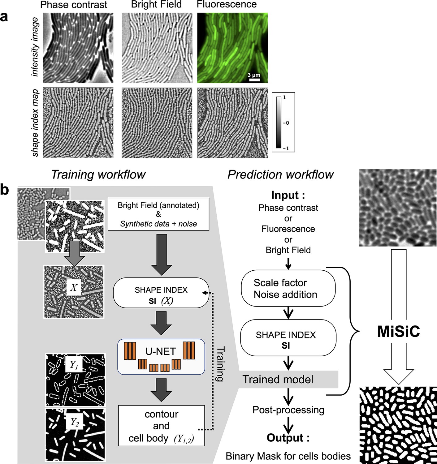
MiSiC: A U-netbased bacteria segmentation tool.
(a) Examples of Shape index maps (SI) calculated from Phase Contrast, Bright Field and Fluorescence images of the same field of Myxococcus xanthus cells. (b) A set of annotated bright-field images of Escherichia coli and Myxococcus xanthus along with synthetic labeled data with additive Gaussian noise was used to generate a training dataset of input images, X, consisting of Shape Index Map of intensity images (at three scales) and segmented images, Y, consisting of contours (Y1) and cell body (Y2). A CNN with U-net architecture was trained to segment the Shape Index Maps into cell body and contour of bacterial cells. Prediction using MiSiC requires that the mean width of the bacteria in the input image is close to 10 pixels, which is easily obtained by rescaling the input image based on the average width of the bacteria under consideration. Gaussian noise may be added to the input image to reduce false positives (Materials and methods).
Figure 1—figure supplement 1
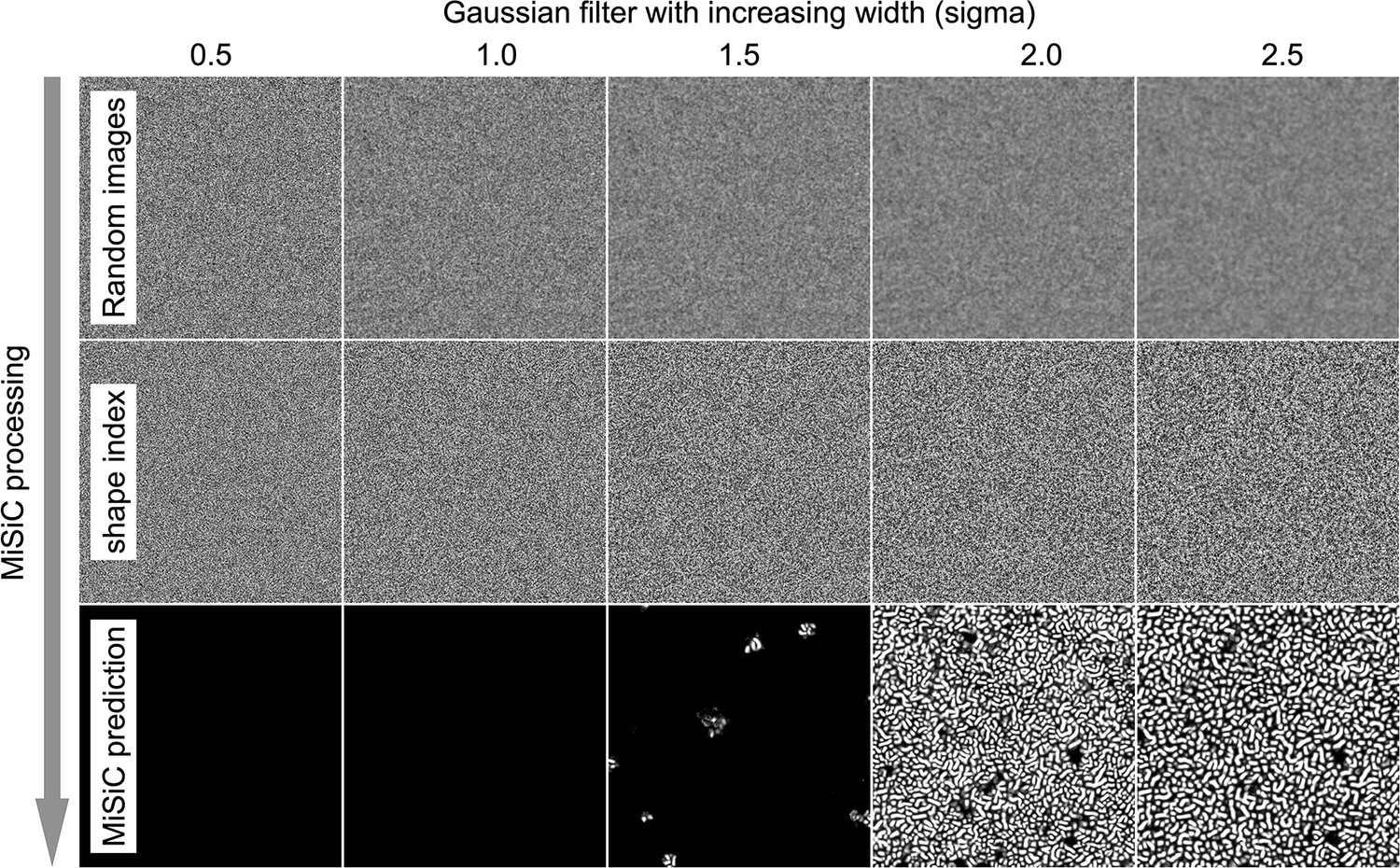
Background noise can lead to spurious cell detection by MiSiC.
SI images retain the shape/curvature information of the intensities in a raw image through eigenvalues of the hessian of the image and an arctan function, creating the smooth areas corresponding to cell bodies and propagating noisy regions where there is no shape information. Thus, MiSiC segments the cells by discriminating between ‘smooth’ and ‘rough’ regions. In effect, when adjusting the size parameter, scaling smooths out the image noise, leading to background regions that have a smoother SI than in the raw image. Some of these areas could be falsely detected as bacterial cells. This effect is shown here: When an image with uniform and random intensity values is segmented with MiSiC with increasing smoothening (here using a gaussian blur filter), spurious cell detection becomes apparent. In addition, since the SI keeps the shape information and not the intensity values, background objects that are of relatively low contrast (i.e. dead cells or debris) may be detected as cells. All these artifacts can be mitigated by adding synthetic noise to the scaled images.
Figure 2 with 1 supplement
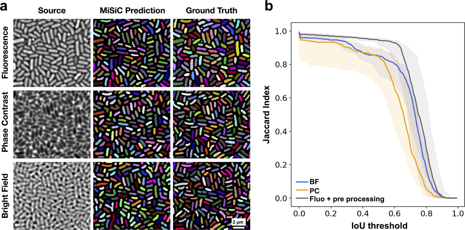
MiSiC predictions under various imaging modalities.
(a) MiSiC masks and corresponding annotated masks of fluorescence, phase contrast and bright field images of a dense E. coli microcolony. (b) Jaccard index as a function of IoU threshold for each modality determined by comparing the MiSiC masks to the ground truth (see Materials and methods). The obtained Jaccard score curves are the average of analyses conducted over three biological replicates and n = 763, 811, 799 total cells for Fluorescence, Phase Contrast and Bright Field, respectively (bands are the maximum range, the solid line is the median). The fluorescence images were pre-processed using a Gaussian of Laplacian filter to improve MiSiC prediction (describe in Materials and methods).
-
Figure 2—source data 1
E. coli IoU over threshold -Brightfield.
- https://cdn.elifesciences.org/articles/65151/elife-65151-fig2-data1-v2.csv
-
Figure 2—source data 2
E. coli IoU over threshold -Fluorescence.
- https://cdn.elifesciences.org/articles/65151/elife-65151-fig2-data2-v2.csv
-
Figure 2—source data 3
E. coli IoU over threshold – Phase contrast.
- https://cdn.elifesciences.org/articles/65151/elife-65151-fig2-data3-v2.csv
Figure 2—figure supplement 1

MiSiC predictions under various imaging modalities.
(a) MiSiC masks and corresponding annotated masks of fluorescence, phase contrast and bright-field images of a dense M. xanthus microcolony. (b) Jaccard index as a function of IoU threshold for each modality determined by comparing the MiSiC masks to the ground truth (see Materials and methods). The obtained curves are the average of analyses conducted over three biological replicates and n = 193,206,211 total cells for Fluorescence, Phase Contrast, and Bright Field, respectively. The fluorescence (bands are the maximum range, the solid line is the median) images were pre-processed using a Gaussian of Laplacian filter to improve MiSiC prediction (see Materials and methods). (c) A human observer is slightly less performant than MiSiC. The same ground truth as used in Figure 2 (dashed lines) was compared to an independent observer’s annotation (solid lines) and Jaccard score curves were constructed as shown in Figure 2. BF: Bright Field, PC: Phase Contrast, Fluo: Fluorescence.
-
Figure 2—figure supplement 1—source data 1
Myxococcus IoU over threshold -Brightfield for panel b.
- https://cdn.elifesciences.org/articles/65151/elife-65151-fig2-figsupp1-data1-v2.csv
-
Figure 2—figure supplement 1—source data 2
Myxococcus IoU over threshold -Phase Contrast for panel b.
- https://cdn.elifesciences.org/articles/65151/elife-65151-fig2-figsupp1-data2-v2.csv
-
Figure 2—figure supplement 1—source data 3
Myxococcus IoU over threshold-Fluorescence for panel b.
- https://cdn.elifesciences.org/articles/65151/elife-65151-fig2-figsupp1-data3-v2.csv
-
Figure 2—figure supplement 1—source data 4
Threshold for panel 1 c.
- https://cdn.elifesciences.org/articles/65151/elife-65151-fig2-figsupp1-data4-v2.csv
-
Figure 2—figure supplement 1—source data 5
Ground truth IoU over threshold-Brightfield for panel c.
- https://cdn.elifesciences.org/articles/65151/elife-65151-fig2-figsupp1-data5-v2.csv
-
Figure 2—figure supplement 1—source data 6
Ground truth IoU over threshold-Phase contrast for panel c.
- https://cdn.elifesciences.org/articles/65151/elife-65151-fig2-figsupp1-data6-v2.csv
-
Figure 2—figure supplement 1—source data 7
Ground truth IoU over threshold-Fluorescence for panel c.
- https://cdn.elifesciences.org/articles/65151/elife-65151-fig2-figsupp1-data7-v2.csv
-
Figure 2—figure supplement 1—source data 8
Observer IoU over threshold-Brightfield for panel c.
- https://cdn.elifesciences.org/articles/65151/elife-65151-fig2-figsupp1-data8-v2.csv
-
Figure 2—figure supplement 1—source data 9
Observer IoU over threshold-Phase contrast for panel c.
- https://cdn.elifesciences.org/articles/65151/elife-65151-fig2-figsupp1-data9-v2.csv
-
Figure 2—figure supplement 1—source data 10
Observer IoU over threshold-Fluorescence for panel c.
- https://cdn.elifesciences.org/articles/65151/elife-65151-fig2-figsupp1-data10-v2.csv
Figure 3 with 1 supplement
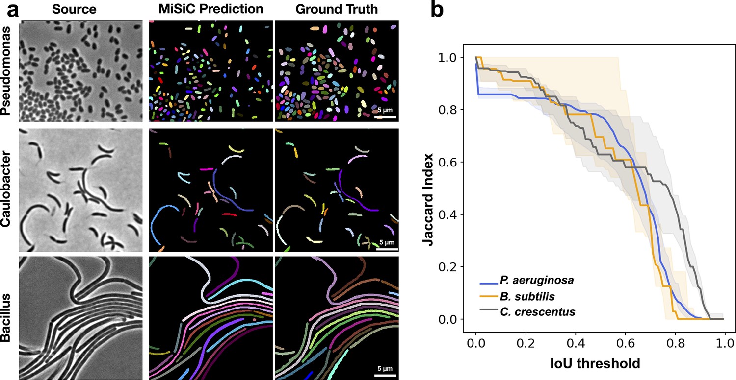
MiSiC predictions in various bacterial species and shapes.
(a) MiSiC masks and corresponding annotated masks of phase contrast images of another Pseudomonas aeruginosa (rod-shape), Caulobacter crescentus (crescent shape) and Bacillus subtilis (filamentous shape). (b) Jaccard index as a function of IoU threshold for each species determined by comparing the MiSiC masks to the ground truth (see Materials and methods). The obtained Jaccard score curves are the average of analyses conducted over three biological replicates and n = 1149,101, 216 total cells for P. aeruginosa, B. subtilis and C. crescentus, respectively (bands are the maximum range, solid line the median). Note that the B. subtilis filaments are well predicted but edge information is missing for optimal detection of the cell separations.
-
Figure 3—source data 1
IoU over threshold -Bacillus subtilis.
- https://cdn.elifesciences.org/articles/65151/elife-65151-fig3-data1-v2.csv
-
Figure 3—source data 2
IoU over threshold -Caulobacter crescentus.
- https://cdn.elifesciences.org/articles/65151/elife-65151-fig3-data2-v2.csv
-
Figure 3—source data 3
IoU over threshold – Pseudomonas aeruginosa.
Thresholds are the same in Figure 2.
- https://cdn.elifesciences.org/articles/65151/elife-65151-fig3-data3-v2.csv
Figure 3—figure supplement 1
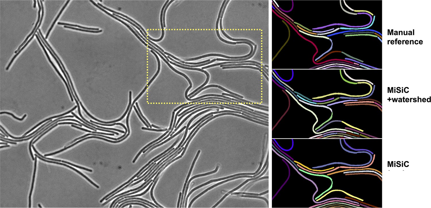
Refining cell separations with watershed.
Watershed methods may be used to obtain a more accurate segmentation of septate filaments such as Bacillus subtilis. In this example, applying this method to the MiSiC mask effectively resolves cell boundaries that are not captured in the prediction but are visible by eye (arrows).
Figure 4 with 1 supplement
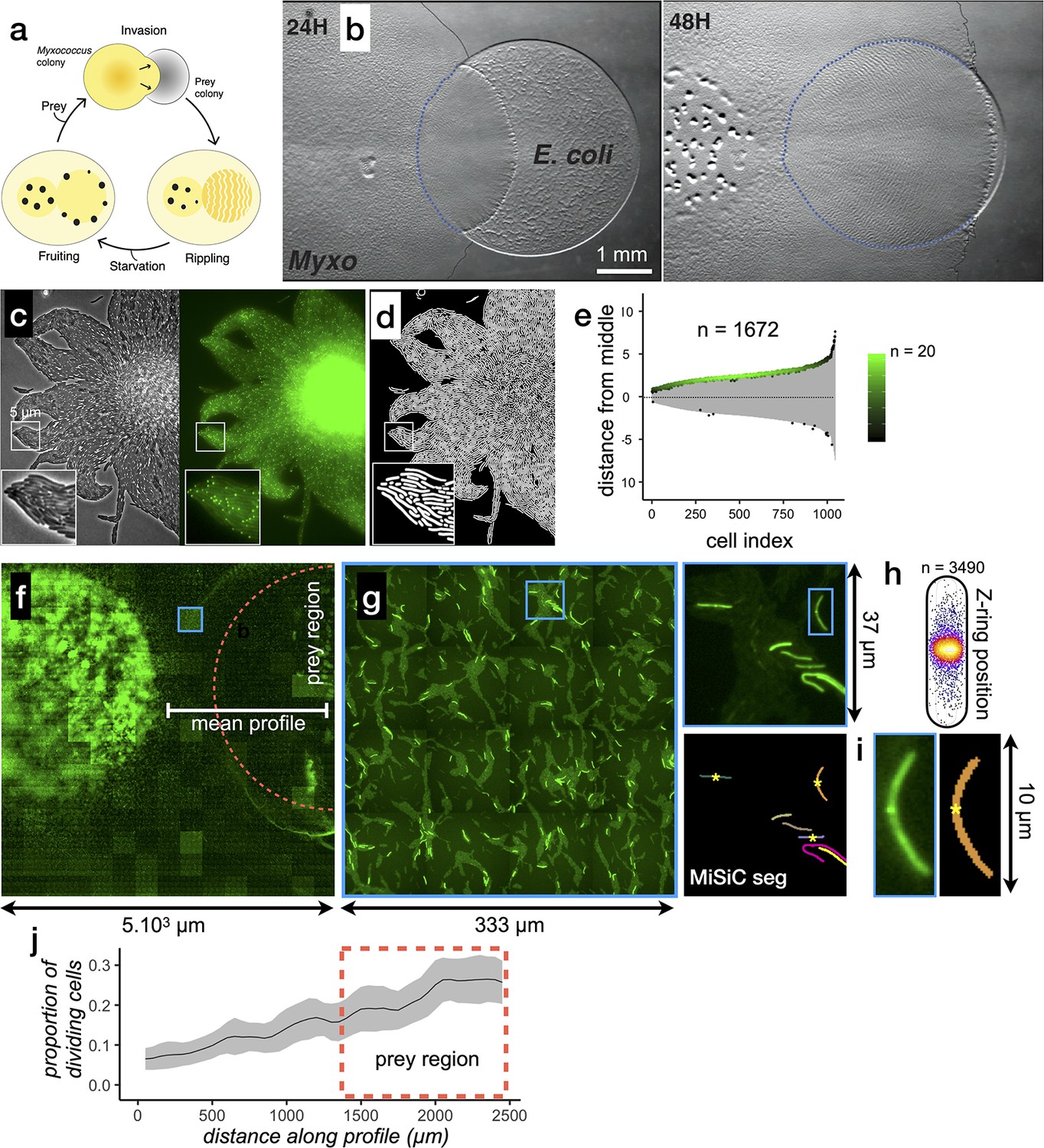
MiSiC can be applied to the study of cellular processes at the mesoscale.
(a) The Myxococcus xanthus predation cycle. Myxococcus cells use motility (yellow colony) to form so-called rippling waves to invade and consume prey colonies (gray). When encountering starvation (outside the prey) or after the prey is consumed, the Myxcococcus cells form aggregate that matures into fruiting bodies (black dots) where the cells differentiate into spores. These spores remain dormant until another prey is encountered which provokes the cycle to resume (see Pérez et al., 2016 for details about the cycle).(b) The Myxococcus xanthus cycle can be observed directly on a Petri dish. Shown are 24 H and 48 H time points. At 48 H, spore-filled fruiting bodies are observed forming in the nutrient depleted area but not in the former prey area where the Myxococcus cells are actively growing. This stage corresponds to the rippling stage shown in (a). Scale bar = 0.5 mm. (c–e) MiSiC can segment dense bacterial swarms.(c) An M. xanthus swarm expressing SgmX-GFP, observed at colony edges and captured under phase contrast, fluorescence and corresponding magnified images.(d) MiSiC prediction mask obtained on the phase contrast image shown in b (e) Demograph representation of the segmented cells in the MiSiC mask (d) and corresponding localization of the SgmX-GFP fluorescent clusters. The horizontal axis represents the number of cells ordered by cell length. The vertical axis represents cell coordinates in µm and aligned such that polar fluorescence clusters have positive values (with respect to the position of the cell middle set to 0). The color of the clusters reflects the number of cells for each given cell length (bins = 0.05 µm, maximum = 20 cells for [3.9–3.95] µm). n = 1672 detected cells after filtering the MiSiC mask. (f–j) Mapping of M. xanthus cell division in the M. xanthus-E. coli community. (f–g) Bacto-Hubble image of a predatory field containing FtsZ-NG labeled Myxococcus xanthus cells and unlabeled Escherichia coli prey cells. The composite image results from the assembly of 15 × 15 Tile images. The dotted circle marks the limits of the original prey colony. The white line (mean profile) indicates the axis used for the analysis shown in (i). (f), a single image tile showing a representative density of fluorescent cells. (h) Detection of dividing cells. FtsZ-NG fluorescent clusters are detected at midcell. The FtsZ clusters can be detected as fluorescence intensity maxima. Shown is a projection of the position of fluorescence intensity on a mean cell contour for a subset of n = 3490 cells (representing 14 % of the total detected cells with a cluster), revealing that as expected, the clusters form at mid-cell. The blue square marks the cell shown as an example in (h). (i) Counting dividing cells. The example shows segmentation of the field shown in (h). The position of Z-ring foci detected as fluorescent maxima was linked to all fluorescent cells segmented in the MiSiC mask. (j) Myxococcus cells divide in the prey colony. The spatial density of dividing cells, the total fluorescent cells (Materials and methods) and the proportion of dividing cells (density of dividing cells/density of total cells, Materials and methods) were determined all across the prey area shown in (e) (dotted circle). The mean ratio and standard deviation are plotted along a spatial axis (distance along profile) corresponding to areas outside and inside (dotted rectangle) of the prey area (mean profile, white segment in (e)).
-
Figure 4—source data 1
Fluorescence maxima – Figure 4e.
- https://cdn.elifesciences.org/articles/65151/elife-65151-fig4-data1-v2.csv
-
Figure 4—source data 2
Cell length – Figure 4e.
- https://cdn.elifesciences.org/articles/65151/elife-65151-fig4-data2-v2.csv
-
Figure 4—source data 3
Z-ring positioning for Figure 4h.
- https://cdn.elifesciences.org/articles/65151/elife-65151-fig4-data3-v2.csv
Figure 4—figure supplement 1

Bacto-Hubble captures millimeter size images of bacterial communities which can be segmented with MiSiC.
(a) Bacto-hubble microscope set-up. The inverted microscope and the sample holder have been optimized to increase the speed of tile acquisition and the stability of focus. The key point is to replace as many moving parts as possible, such as shutters, and replace them with diode sources. The agar pad is blocked by a flat coverslip that, combined with the continuous focus control (in our case a Nikon PFS system), makes it possible to maintain the focus over millimeter and up to centimeter distances. The motorized stage is equipped with optical encoders, allowing precise x, y movements across the specimen. (b) Bacto-Hubble image of an entire predator-prey colony. The area shows an M. xanthus community 96 hours after it started invading an E. coli prey colony. At this stage, the prey has been entirely consumed. Following growth and starvation, M. xanthus cells aggregate (phase-bright dots in the image, top panels) and form fruiting bodies. The entire image corresponds to the assembly of 40 × 40 tiles for a total surface of 9 mm2. Top right panel is a close up of the region framed in light blue in the top left panel. Bottom left panel is a close up of the region framed in yellow in the top right panel. Bottom right panel is a close up of the region framed in red in the bottom left panel showing individual M. xanthus cells. (c–d) Robustness of MiSiC to noise and comparison with SuperSegger. (d) Resulting images with added noise and corresponding segmentation with MiSiC and SuperSegger for comparison. An E. coli dataset was processed with SuperSegger and MiSiC in the presence of increasing amounts of Gaussian noise added to the images while keeping segmentation parameters constant (Materials and methods). (e) Relative performance of SuperSegger and MiSiC to increasing noise. For each amount of noise, the complete datasets (141 images) were processed and the Dice index (Materials and method) was calculated with respect to the segmentation results (ie panel D). Each dot on the lines represents the mean Dice value while the shaded error bars represent its standard deviation across the dataset. Note that while Superseger and MiSiC perform equally well at low noise on this data set (a Supersegger optimized dataset, Materials and methods), MiSiC remains robust in the presence of noise, showing that it is especially adequate for the segmentation of multi-tile images here noise varies significantly between tiles.
-
Figure 4—figure supplement 1—source data 1
DICE index as a function of noise for panel d.
- https://cdn.elifesciences.org/articles/65151/elife-65151-fig4-figsupp1-data1-v2.xlsx
Figure 5
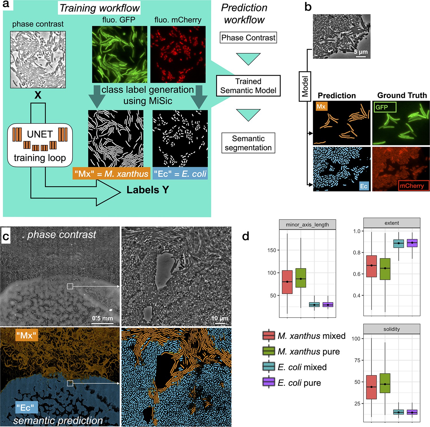
Semantic segmentation of M. xanthus and E. coli from single phase contrast images.
(a) Semantic classification network. A U-Net was trained to discriminate M. xanthus cells from E. coli cells. The training dataset consisted of GFP+ M. xanthus cells mixed with mCherry+ E. coli cells, which were imaged in distinct fluorescent channels (GFP and mCherry) and segmented using MiSiC to produce ground truth data for each species. The network uses unlabeled phase contrast images as input (X) and produces one output for each labeled species (Y, Mx or Ec). (b) Semantic classification of intermixed Myxococcus and E. coli cells. Shown is a mixed population of GFP+ Myxococcus and mCherry+ E. coli cells. The classification (Myxococcus, Mx) and E. coli (Ec) were obtained directly from the phase contrast image. Corresponding fluorescence images of GFP+ and mCherry+ are shown for comparison and were used to estimate the accuracy of the classification. (c–d) Direct semantic classification of M. xanthus interacting with E. coli in a Bacto-Hubble image. (c) Bacto-Hubble image of M. xanthus cells invading an E. coli colony after 24 hours. The composite image corresponds to 20 × 42 image tiles captured by phase contrast and segmented tile-by-tile to produce the resulting classification. Inset: zoom of an area where M. xanthus cells interact tightly with E. coli cells within the E. coli colony. Phase Contrast and corresponding predictions (M. xanthus in orange and E. coli in blue) are shown. (d) Morphological analyses of the classified cell population and comparison with the ground truth data. Morphological parameters (Extent, Solidity and minor axis length) were determined for the cells predicted in the M. xanthus (Mx mixed) and E. coli masks (E. coli mixed) in the context of a mixed colony and compared to the same parameters obtained from MiSiC segmented from images of pure cultures (Mx/E. coli pure).
-
Figure 5—source data 1
E. coli only for Figure 5d.
- https://cdn.elifesciences.org/articles/65151/elife-65151-fig5-data1-v2.csv
-
Figure 5—source data 2
E. coli in mixed colony for Figure 5d.
- https://cdn.elifesciences.org/articles/65151/elife-65151-fig5-data2-v2.csv
-
Figure 5—source data 3
M.xanthus only for Figure 5d.
- https://cdn.elifesciences.org/articles/65151/elife-65151-fig5-data3-v2.csv
-
Figure 5—source data 4
M.xanthus in mixed colony for Figure 5d.
- https://cdn.elifesciences.org/articles/65151/elife-65151-fig5-data4-v2.csv
Author response image 1
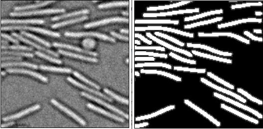
Note the presence of a round object (perhaps a round cell) in the PC image.
MiSiC excludes this object because it deviates too much from the training data set only to retain the rod shape objects.
Additional files
-
Transparent reporting form
- https://cdn.elifesciences.org/articles/65151/elife-65151-transrepform1-v2.docx
-
Supplementary file 1
Table S1 - Bacterial strains used in this study.
- https://cdn.elifesciences.org/articles/65151/elife-65151-supp1-v2.pdf
-
Supplementary file 2
Table S2 - Primers.
- https://cdn.elifesciences.org/articles/65151/elife-65151-supp2-v2.pdf
-
Supplementary file 3
Table S3 - Plasmids.
- https://cdn.elifesciences.org/articles/65151/elife-65151-supp3-v2.pdf
Download links
A two-part list of links to download the article, or parts of the article, in various formats.
Downloads (link to download the article as PDF)
Open citations (links to open the citations from this article in various online reference manager services)
Cite this article (links to download the citations from this article in formats compatible with various reference manager tools)
Misic, a general deep learning-based method for the high-throughput cell segmentation of complex bacterial communities
eLife 10:e65151.
https://doi.org/10.7554/eLife.65151


