Competition between parallel sensorimotor learning systems
- Department of Biomedical Engineering, Johns Hopkins School of Medicine, United States
- Neuroscience Center, University of North Carolina, United States
- Vanderbilt University School of Medicine, United States
- Department of Kinesiology and Health Science, York University, Canada
- IFIBIO Houssay, Deparamento de Fisiología y Biofísia, Facultad de Medicina, Universidad de Buenos Aires, Argentina
- Department of Neurology, Johns Hopkins School of Medicine, United States
- Department of Neuroscience, Johns Hopkins School of Medicine, United States
- The Santa Fe Institute, United States
Figures
Figure 1 with 4 supplements
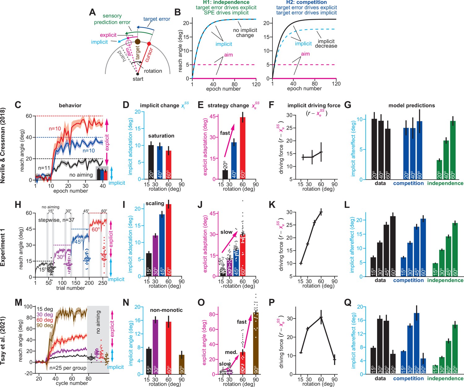
Total implicit learning is shaped by competition with explicit strategy.
(A). Schematic of visuomotor rotation. Participants move from start to target. Hand path is composed of explicit (aim) and implicit corrections. Cursor path is perturbed by rotation. We explored two hypotheses: prediction error (H1, aim vs. cursor) vs. target error (H2, target vs. cursor) drives implicit learning. (B) Prediction error hypothesis predicts that enhancing aiming (dashed magenta) will not change implicit learning (black vs. dashed cyan) according to the independence equation. Target error hypothesis predicts that enhancing aiming (dashed magenta) will decrease implicit adaptation (black vs. dashed cyan). (C) Data reported by Neville and Cressman, 2018. Participants were exposed to either a 20°, 40°, or 60° rotation. Learning curves are shown. The “no aiming” inset shows implicit learning measured via exclusion trials at the end of adaptation. Explicit strategy was calculated as the voluntary reduction in reach angle during the no aiming period. (D) Implicit learning measured during no aiming period in Neville and Cressman yielded a ‘saturation’ phenotype. (E) Explicit strategies calculated in Neville & Cressman dataset by subtracting exclusion trial reach angles from the total adapted reach angle. (F) The implicit learning driving force in the competition theory: difference between rotation and explicit learning in Neville and Cressman. (G) Implicit learning predicted by the competition and independence models in Neville and Cressman. Models were fit assuming that the implicit learning gain was identical across rotation sizes. (H) Experiment 1. Subjects in the stepwise group (n = 37) experienced a 60° rotation gradually in four steps: 15°, 30°, 45°, and 60°. Implicit learning was measured via exclusion trials (points) twice in each rotation period (gray ‘no aiming’). (I) Total implicit learning calculated during each rotation period in the stepwise group yielded a ‘scaling’ phenotype. (J) Explicit strategies were calculated in the stepwise group by subtracting exclusion trial reach angles from the total adapted reach angle. (K) The implicit learning driving force in the competition theory: difference between rotation and explicit learning in the stepwise group. (L) Implicit learning predicted by the competition and independence models in the stepwise group. Models were fit assuming that implicit learning gain was constant across rotation size. (M) Data reported by Tsay et al., 2021a. Participants were exposed to either a 15°, 30°, 60°, or 90° rotation. Learning curves are shown. The “no aiming” inset shows implicit learning measured via exclusion trials at the end of adaptation. (N) Implicit learning measured during no aiming period in Tsay et al. yielded a ‘non-monotonic’ phenotype. (O) Explicit strategies calculated in Tsay et al. dataset by subtracting exclusion trial reach angles from the total adapted reach angle. (P) Implicit learning driving force in the competition theory: difference between rotation and explicit learning in Tsay et al. (Q) Total implicit learning predicted by the competition and independence models in Tsay et al. Models were fit assuming that the implicit learning gain was identical across rotation sizes. Error bars show mean ± SEM, except in the independence predictions in G, L, and Q; independence predictions show mean and standard deviation across 10,000 bootstrapped samples. Points in H, J, M, and O show individual participants.
-
Figure 1—source code 1
Figure 1 data and analysis code.
- https://cdn.elifesciences.org/articles/65361/elife-65361-fig1-code1-v2.zip
Figure 1—figure supplement 1
Implicit learning can exhibit various phenotypes in the competition theory.
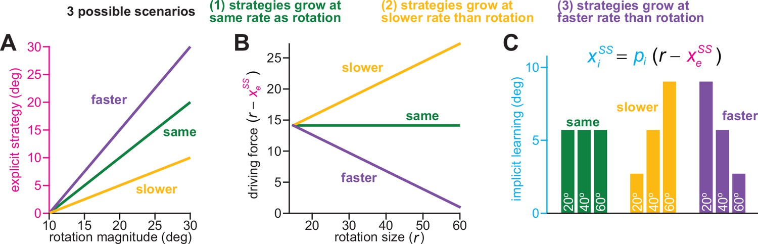
Here we consider how implicit learning can respond to changes in rotation size in the competition theory. (A) Total implicit learning in the competition theory is altered by explicit strategy. We show three cases: (1) strategy increases at the same rate as rotation size (‘same’, gain = 1), (2) strategy increases more slowly than rotation size (‘slower’, gain <1), (3) strategy increases faster than rotation size (‘faster’, gain >1). Gain here is equal to each line’s slope (it is not dependent on the intercept, which is non-zero). (B) In the competition theory, the driving input to the implicit system is the error (i.e. difference) between the rotation and steady-state explicit strategy. Thus, when explicit strategy and rotation size grow by the same amount (‘same’), the implicit driving force remains constant. When explicit strategy grows more than the rotation (“faster”), the implicit driving force decreases as the rotation gets larger. When explicit strategy grows less than the rotation (“slower”), the implicit driving force increases as the rotation gets larger. (C) In the competition theory (equation at top), implicit learning is proportional to the implicit driving forces depicted in B. The proportionality constant, pi, depends on implicit error sensitivity and retention (see Equation 4). Thus, in the ‘same’ scenario in A and B, implicit learning will remain the same across rotation sizes. In the ‘slower’ scenario in A and B, implicit learning will increase with the rotation. In the ‘faster’ scenario in A and B, implicit learning with decrease as the rotation increases.
Figure 1—figure supplement 2
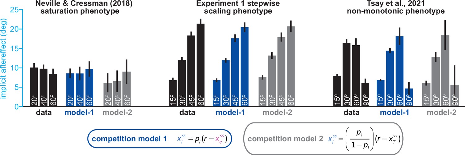
Variations between total learning and implicit learning are consistent with the competition model.
In Figure 1, we evaluate how well the competition equations matches data across three distinct implicit learning phenotypes: saturation, scaling, and non-monotonic responses. These three implicit learning phenotypes are shown again here (data, black bars; each group from left to right shows a different phenotype). The competition model is intuitively stated as a relationship between implicit learning and explicit strategy. This equation is denoted in blue: ‘competition model 1’. Blue bars show how much implicit learning was predicted in each experiment, using explicit strategy and ‘competition model 1’ (‘model-1’ under each set of bars). The competition model can be stated another way. Noting that total adaptation is equal to the sum of implicit and explicit learning, we can replace explicit learning in ‘competition model 1’, with total adaptation minus implicit learning. Algebraic simplification yields ‘competition model 2’, shown in gray. This is an equivalent competition model, only this time, it is stated as a relationship between implicit learning and total adaptation (which were measured on separate trials). The gray bars (‘model-2’) show how much implicit learning was predicted by ‘competition model 2’, using measured total adaptation. Competition models 1 (implicit predicted using explicit) and 2 (implicit predicted using total adaptation) yielded nearly identical predictions. More detail on these comparisons is provided in Appendix 3.
-
Figure 1—figure supplement 2—source code 1
Figure 1—figure supplement 2 data and analysis code.
- https://cdn.elifesciences.org/articles/65361/elife-65361-fig1-figsupp2-code1-v2.zip
Figure 1—figure supplement 3
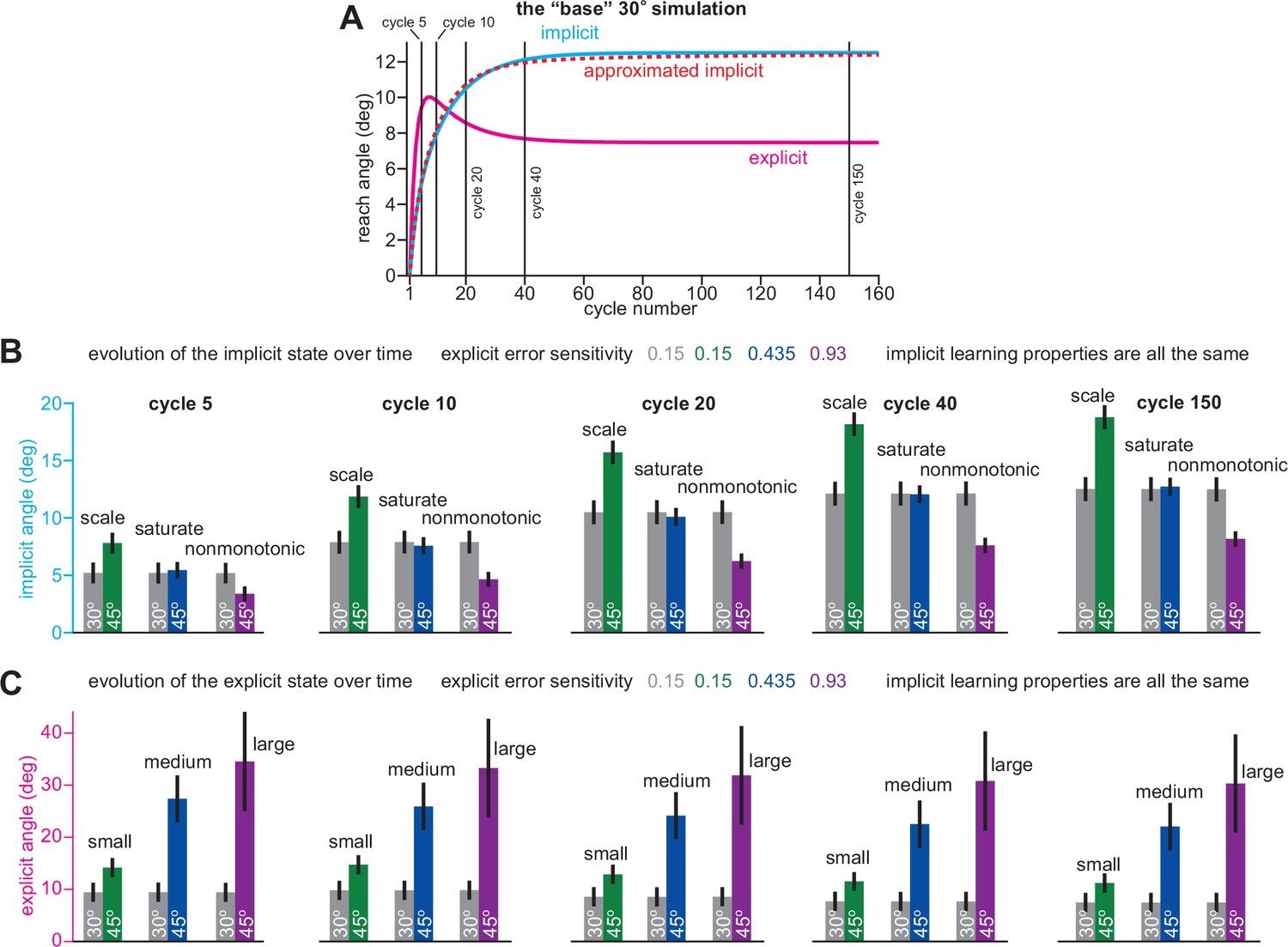
Scaling, saturation, and non-monotonic phenotypes across the implicit learning timecourse.
(A) A ‘base’ simulation where implicit and explicit systems adapt to target error. A response to a 30° rotation is shown. This response matches the gray bars in B and C. Note the vertical lines. These indicate moments in time where the implicit and explicit responses were calculated in B and C: from left to right, 5, 10, 20, 40, and 150 rotation cycles. Also note the red dashed ‘approximated implicit’ line. This shows the implicit approximation detailed in Appendix 1.1, where xe is replaced with the average explicit strategy up until that cycle number. In B and C we show implicit and explicit responses measured at each vertical bar in A. Left to right shows the early-to-late evolution of each adaptive process. (B) shows implicit learning. (C) shows explicit learning. Green, blue, and purple bars correspond to a 45° rotation response. In addition to changing the rotation magnitude, explicit error sensitivity was also modulated to create the scaling, saturation, and nonmonotonic implicit learning modes. In green, be remained at 0.15 (the same as the gray ‘base’ simulation). In blue, be was increased to 0.435. In purple, be was increased dramatically to 0.93. The scale, saturate, and nonmonotonic phenotypes can be seen at all timepoints in B.
-
Figure 1—figure supplement 3—source code 1
Figure 1—figure supplement 3 analysis code.
- https://cdn.elifesciences.org/articles/65361/elife-65361-fig1-figsupp3-code1-v2.zip
Figure 1—figure supplement 4
Changes in implicit learning across blocks.
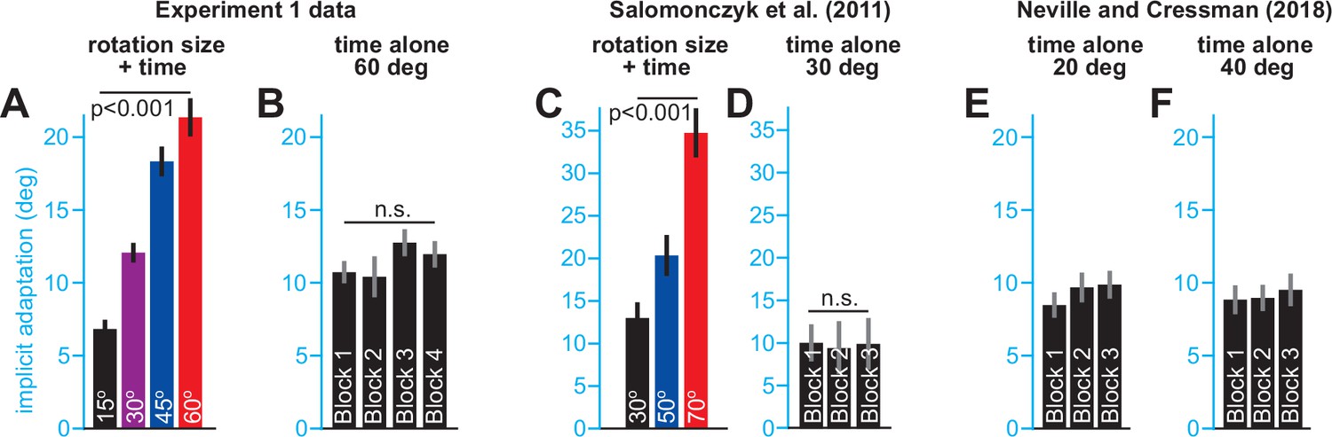
(A) Implicit learning measured during each block in the stepwise group in Exp. 1. (B) Implicit learning measured during each block in the abrupt group in Exp. 1. (C) Implicit learning measured in a stepwise condition in Salomonczyk et al., 2011. (D) Implicit learning measured in a 30° group over three learning blocks in Salomonczyk et al., 2011. (E) Implicit learning measured in a 20° group over three learning blocks in Neville and Cressman, 2018. (F) Same as E, but for a 40° group.
-
Figure 1—figure supplement 4—source code 1
Figure 1—figure supplement 4 data and analysis code.
- https://cdn.elifesciences.org/articles/65361/elife-65361-fig1-figsupp4-code1-v2.zip
Figure 2 with 4 supplements
Increases or decreases in explicit strategy oppositely impact implicit adaptation.
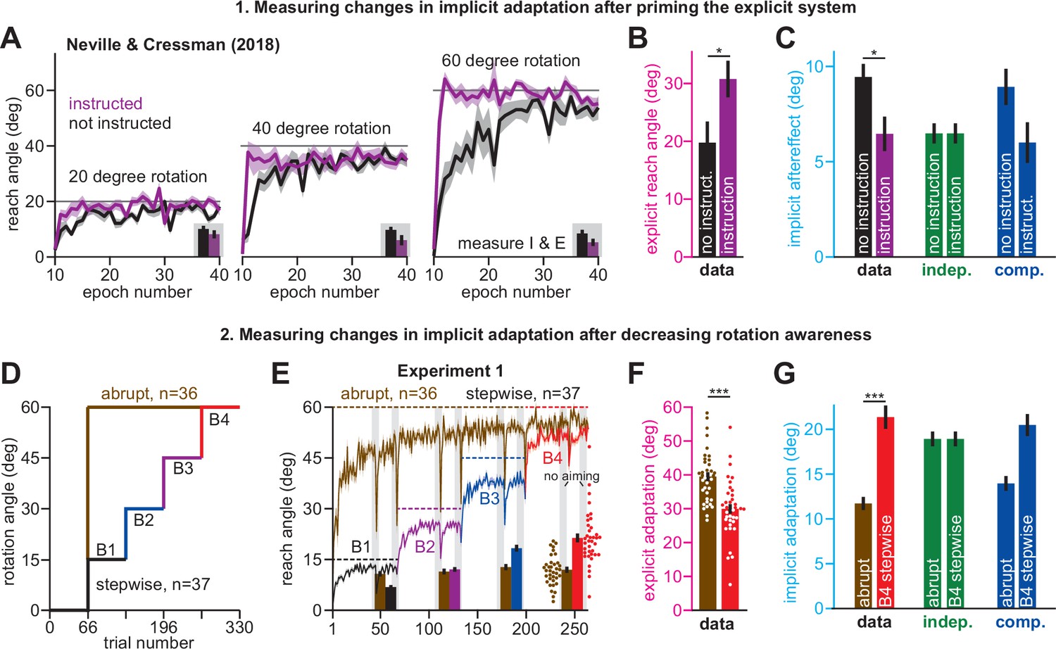
(A) Neville and Cressman, 2018 tested participants in two conditions: an uninstructed condition (black) and an instructed condition (purple) where subjects were briefed about the upcoming rotation and its solution. Instruction increased the adaptation rate across three rotation sizes: 20°, 40°, and 60°. Insets in gray shaded area show implicit adaptation measured via exclusion trials at the end of adaptation. (B) Here, we show the average strategy across all rotation sizes in the instructed (black) and uninstructed (purple) conditions. Explicit strategy was calculated by subtracting implicit learning (exclusion trials) from total adaptation. Instruction increased explicit strategy use. (C) The data show implicit adaptation averaged across all three rotation sizes. The independent (SPE learning) and competition (target error learning) models were fit to these data assuming that implicit error sensitivity and retention were identical across rotation sizes and instruction conditions (i.e. identical ai and bi across all six groups). Error bars for model predictions refer to mean and standard deviation across 10,000 bootstrapped samples. (D) In Experiment 1 we tested participants in either an abrupt condition or a stepwise (gradual) condition. Here, we show the rotation schedule. (E) Here, we show learning curves in the abrupt and stepwise conditions in Experiment 1. Bars show implicit adaptation measured during each rotation period (four blocks total) via exclusion trials. Individual learning measures are shown in the terminal 60° learning period for both groups (points at bottom-right). (F) We calculated explicit strategies during the terminal 60° learning period by subtracting implicit learning measures from total adaptation (mean over last 20 trials). Gradual onset reduced explicit strategy use. (G) The data show total implicit learning measured in the 60° rotation period. The competition (blue) and independence (green) models were fit to the data assuming that the implicit learning parameters were the same across the abrupt and stepwise groups. Error bars for the model show the mean and standard deviation across 1,000 bootstrapped samples. Statistics in B, F, and G denote a two-sample t-test: *p < 0.05, ***p < 0.001. Error bars in A, B, C (data), E, F, and G (data) denote mean ± SEM. Points in E and F show individual participants.
-
Figure 2—source code 1
Figure 2 data and analysis code.
- https://cdn.elifesciences.org/articles/65361/elife-65361-fig2-code1-v2.zip
Figure 2—figure supplement 1
Changes in implicit adaptation in response to awareness and rotation size.
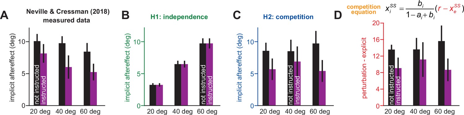
Data reported from Neville and Cressman, 2018. (A) Participants were separated into 1 of 6 groups. Groups differed based on verbal instruction (instructed purple; non-instructed black) and rotation magnitude (20° left; 40° middle; 60° right). Here, we show implicit learning measured using exclusion trials (reach without re-aiming) at the end of adaptation. (B) Here, we show implicit aftereffects predicted by a model where implicit system learns from SPE only. (C) Here we show implicit aftereffects predicted by a model where implicit system learns from target error only. (D). The competition theory (target error learning) predicts that implicit learning will be proportional to the difference between the rotation size and the total explicit strategy. Here we show this quantity for all six experimental groups. Note that model predictions in B and C assume that the implicit learning gain is the same across all six experimental groups. Error bars for data show mean ± SEM. Error bars for model predictions refer to mean and standard deviation across 10,000 bootstrapped samples.
-
Figure 2—figure supplement 1—source code 1
Figure 2—figure supplement 1 data and analysis code.
- https://cdn.elifesciences.org/articles/65361/elife-65361-fig2-figsupp1-code1-v2.zip
Figure 2—figure supplement 2
Total implicit adaptation varies slowly with changes in implicit error sensitivity.
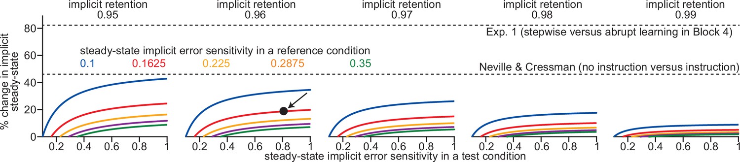
We used a sensitivity analysis to explore whether changes in error sensitivity could explain the variations in implicit learning in Exp. 1 (abrupt vs. stepwise) and Neville and Cressman (instruction vs. no instruction). Above we compare a ‘reference’ and a ‘test’ condition. We chose several possible implicit error sensitivity and retention levels in our ‘reference’. From left to right, we test implicit retention factors between 0.95 and 0.99. The colors in each inset, denote different reference error sensitivities: from 0.1 to 0.35. Each curve shows how much implicit learning will increase in a ‘test’ condition (i.e. the y-axis) over the reference condition; y-axis denotes the percent change in total implicit learning and x-axis denotes error sensitivity in the test condition. For example, for the point highlighted by the black arrow in the second column: this point shows that total implicit learning will increase by about 20% (y-axis) in a scenario where implicit retention = 0.96, and implicit error sensitivity increases from 0.1625 (i.e. it is on the red line) in the reference condition to 0.8 (i.e. the x-axis value) in the test condition.
-
Figure 2—figure supplement 2—source code 1
Figure 2—figure supplement 2 analysis code.
- https://cdn.elifesciences.org/articles/65361/elife-65361-fig2-figsupp2-code1-v2.zip
Figure 2—figure supplement 3
Suppressing explicit strategy increases total implicit adaptation.
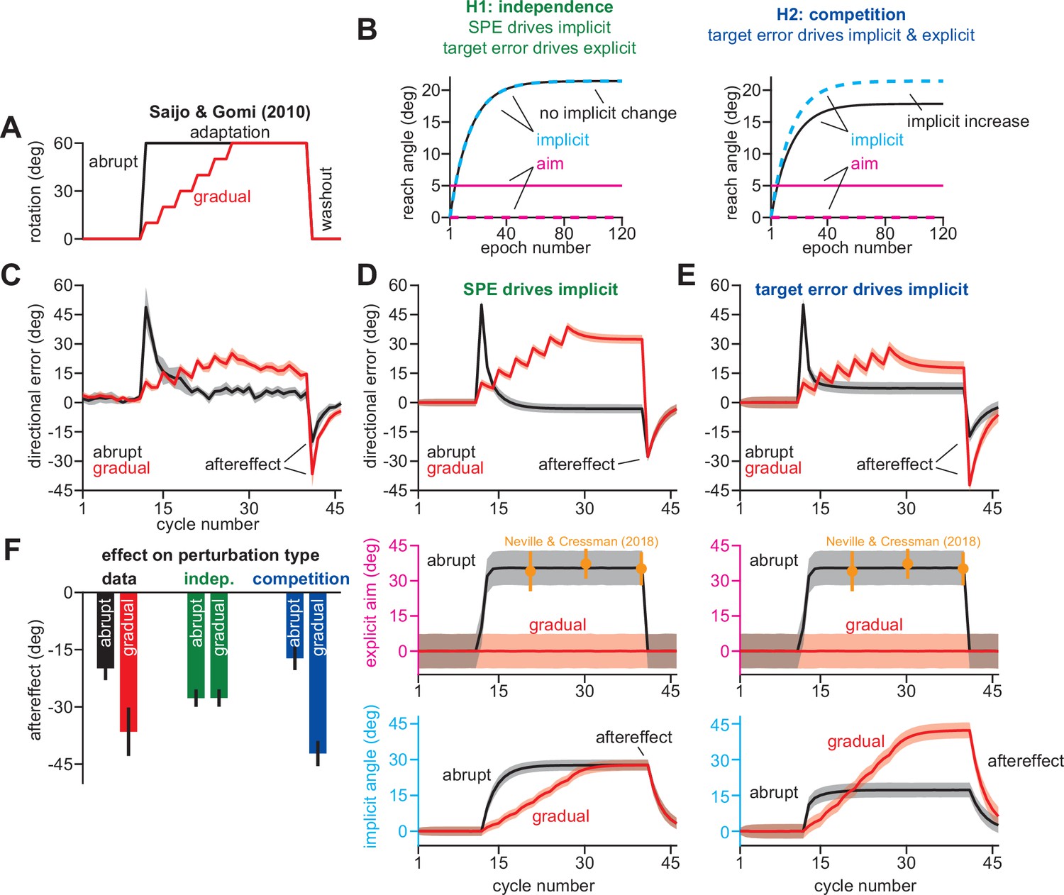
Data reported from Saijo and Gomi, 2010. (A) Participants experienced an abrupt or gradual 60° rotation (followed by washout). (B) We explored two hypotheses: prediction error (H1, aim vs. cursor) vs. target error (H2, target vs. cursor) drives implicit learning. Prediction error hypothesis predicts that suppressing aiming (dashed magenta) through gradual perturbation onset will not change implicit learning (black vs. dashed cyan). Target error hypothesis predicts that suppressing aiming (dashed magenta) will increase implicit adaptation (black vs. dashed cyan). (C) Directional error during adaptation. Note that while the abrupt group exhibited greater adaptation during the rotation, they also showed a smaller aftereffect suggesting less implicit adaptation. (D) We simulated a state-space model where the implicit system learned from SPE. The model parameters were selected to best fit the data in C. In the middle row, hypothetical abrupt explicit strategy was simulated based on data reported by Neville and Cressman, 2018 (yellow points). The gradual explicit strategy was assumed to be zero because participants were less aware. At bottom, we show implicit learning predicted by an SPE error source. Note the identical saturation levels. (E) Same as in D, but for implicit adaptation based on target error. Note greater implicit learning in gradual condition at the bottom row. Models in D and E were fit assuming that implicit error sensitivity and retention are identical across abrupt and gradual conditions. (F) Here, we show the implicit aftereffect on the first washout cycle (12 total trials). Model predictions for SPE learning (indep.) and target error learning (competition) are shown. Data show mean ± SEM across participants. Error bars for model are mean and standard deviation across 20,000 bootstrapped samples.
-
Figure 2—figure supplement 3—source code 1
Figure 2—figure supplement 3 data and analysis code.
- https://cdn.elifesciences.org/articles/65361/elife-65361-fig2-figsupp3-code1-v2.zip
Figure 2—figure supplement 4

The competition model is compatible with various explicit strategy levels in Saijo and Gomi, 2010.
In Appendix 5, we analyzed the Saijo and Gomi, 2010 abrupt and gradual learning conditions with both the competition and independence models. We measured whether each model could predict total implicit learning, with the assumption that the initial washout reach angle primarily reflected implicit adaptation. These analyses assumed that participants in the gradual condition did not use explicit strategy. In the right column, we reproduce the competition model’s predictions under this zero strategy assumption, as in Figure 2—figure supplement 2E and F. Next, we repeated these analyses in an alternate scenario, where explicit strategy was assumed to be 10° during the rotation period. This new control analysis is shown in the left column. We observed that model predictions were qualitatively similar whether gradual learning was simulated with 0° strategy, or 10° strategy. (A) shows directional errors predicted by competition. (B) shows the explicit strategies used as input in these simulations. (C) shows the implicit response to the rotation and explicit strategies predicted by the competition model. (D) shows the aftereffect predicted by the competition model (blue), independence model (green), and that observed in the actual experiment (data). For the model predictions, we used the implicit angle on the initial washout cycle.
-
Figure 2—figure supplement 4—source code 1
Figure 2—figure supplement 4 data and analysis code.
- https://cdn.elifesciences.org/articles/65361/elife-65361-fig2-figsupp4-code1-v2.zip
Figure 3 with 3 supplements
Strategy suppresses implicit learning across individual participants.
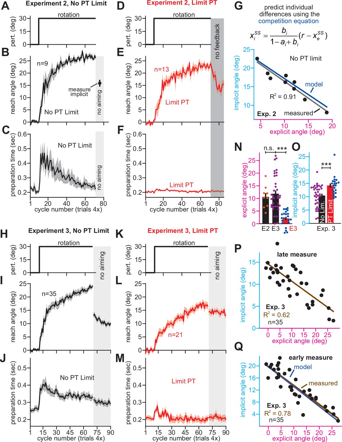
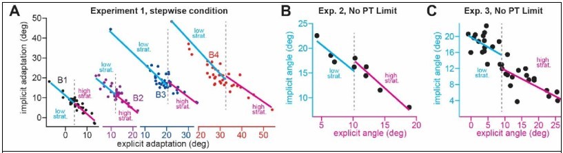
(A–C) In Experiment 2, participants in the No PT Limit (no preparation time limit) group adapted to a 30° rotation. The paradigm is shown in A. The learning curve is shown in B. Implicit learning was measured via exclusion trials (no aiming). Preparation time is shown in C (movement start minus target onset). (D–F) Same as in A–C, but in a limited preparation time condition (Limit PT). Participants in the Limit PT group had to execute movements with restricted preparation time (F). The task ended with a prolonged no visual feedback period where memory retention was measured (E, gray region). (G) Total implicit and explicit adaptation in each participant in the No PT Limit condition (points). Implicit learning measured during the terminal no aiming probe. Explicit learning represents difference between total adaptation (last 10 rotation cycles) and implicit probe. The black line shows a linear regression. The blue line shows the theoretical relationship predicted by the competition equation which assumes implicit system adapts to target error. The parameters for this model prediction (implicit error sensitivity and retention) were measured in the Limit PT group. (H–J) In Experiment 3, participants adapted to a 30° rotation using a personal computer in the No PT Limit condition. The paradigm is shown in H. The learning curve is shown in I. Implicit learning was measured at the end of adaptation over a 20-cycle period where participants were instructed to reach straight to the target without aiming and without feedback (no aiming seen in I). We measured explicit adaptation as difference between total adaptation and reach angle on first no aiming cycle. We measured ‘early’ implicit aftereffect as reach angle on first no aiming cycle. We measured ‘late’ implicit aftereffect as mean reach angle over last 15 no aiming cycles. (K–M) Same as in H–J, but for a Limit PT condition. (N) Explicit adaptation measured in the No PT Limit condition in Experiment 2 (E2), No PT Limit condition in Experiment (E3, black), and Limit PT condition in Experiment 3 (E3, red). (O) Late implicit learning in the Experiment 3 No PT Limit group (No Lim.) and Experiment 3 Limit PT group (PT Limit). (P) Correspondence between late implicit learning and explicit strategy in the Experiment 3 No PT Limit group. (Q) Same as in G but where model parameters are obtained from the Limit PT group in Experiment 3, and points represent subjects in the No PT Limit group in Experiment 3. Early implicit learning is used. Throughout all insets, error bars indicate mean ± SEM across participants. Statistics in N and O are two-sample t-tests: n.s. means p > 0.05, ***p < 0.001.
-
Figure 3—source code 1
Figure 3 data and analysis code.
- https://cdn.elifesciences.org/articles/65361/elife-65361-fig3-code1-v2.zip
Figure 3—figure supplement 1
Implicit error sensitivity varies with error.
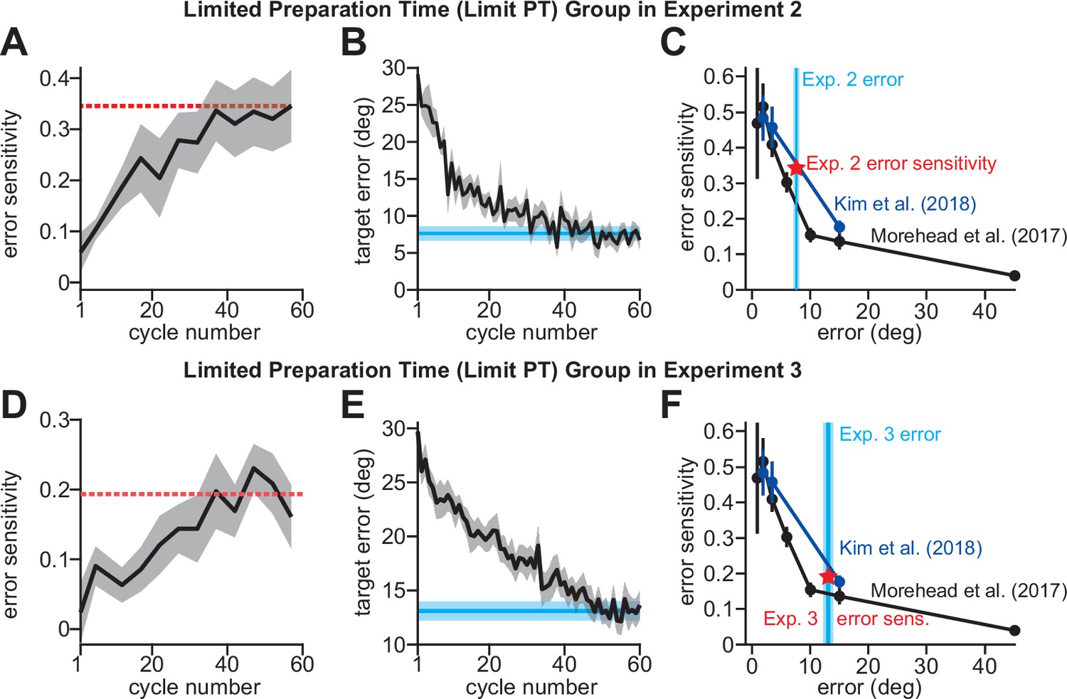
(A) We empirically estimated error sensitivity on each trial in the limited preparation time (Limit PT) group in Experiment 2. The dashed horizontal line indicates the steady-state error sensitivity used in our competition theory predictions in Figure 3G. (B) Here we show error on each trial in the Limit PT group in Experiment 3. The horizontal cyan line shows the terminal error over the last 10 cycles. (C) Error sensitivity curves reported in Kim et al., 2018 denoted E1 (Morehead et al., 2017 results) and E2 (Kim et al., 2018 results). These two studies used invariant error-clamp tasks to isolate implicit learning. We compared our implicit learning measure in the Limit PT condition in Exp. 2 to these values. The vertical blue line shows the terminal error in B. The red star shows the terminal error sensitivity measured in A. In panels D–F, we show the same data as in A–C, except for the Limit PT condition in Experiment three where participants were tested on a personal laptop. Shaded error bars denote mean ± SEM across participants.
-
Figure 3—figure supplement 1—source code 1
Figure 3—figure supplement 1 data and analysis code.
- https://cdn.elifesciences.org/articles/65361/elife-65361-fig3-figsupp1-code1-v2.zip
Figure 3—figure supplement 2

Comparing implicit and explicit adaptation via reported strategies.
In Figure 3, when analyzing the No PT Limit group (no preparation time limit) in Experiment 2, we measured implicit learning using exclusion trials at the end of adaptation. Next, we estimated explicit strategies by subtracting this reach-based implicit learning measure from the total adaptation measured over the last 10 cycles of adaptation (reach-based explicit measure). In addition, we also asked participants to report their explicit strategies after the probe period. Participants were shown a ring of circles surrounding each target and asked to indicate which circle best represented their aiming direction at the end of the experiment. We averaged this report-based explicit measure across all four adaptation targets, taking the absolute value for any misreported strategies (25% of all reports in opposite direction). We estimated report-based implicit learning by subtracting the reported explicit strategy from the total adaptation measured over the last 10 rotation cycles. (A) Here, we compare report-based explicit strategy with reach-based explicit strategy. Each point represents an individual participant. The solid line is the unity line. The bars at right show the mean value for each explicit measure. (B) Similar to A except here we compare report-based implicit learning with reach-based implicit learning. (C) Here we compared report-based implicit and report-based explicit learning measures. We also show the relationship predicted by the competition theory in blue (same as in Figure 3G). Error bars show mean ± SEM across participants. Statistics in A and B show paired t-tests: *p < 0.05.
-
Figure 3—figure supplement 2—source code 1
Figure 3—figure supplement 2 data and analysis code.
- https://cdn.elifesciences.org/articles/65361/elife-65361-fig3-figsupp2-code1-v2.zip
Figure 3—figure supplement 3

Movement paths in Experiment 3 were straight and brisk.
In Exp. 3, we tested participants remotely in a laptop-based rotation study. Here, we show movement paths recorded by the computer in two example subjects: one in the Limit PT group (top row) and one in the No PT Limit group (bottom row). The left column shows trajectories during the baseline period. Note the four different groupings reflect the four different targets used in the task. The middle column shows trajectories during the rotation period. The color indicates the rotation trial number (blue is early in the rotation period, red is late in the rotation period). The data show a clear rotation in participant movement angle. Reach trajectories remained straight. Finally, the right column shows movement paths during the terminal period where participants were instructed to move straight to each target, without any cursor feedback.
-
Figure 3—figure supplement 3—source code 1
Figure 3—figure supplement 3 data and analysis code.
- https://cdn.elifesciences.org/articles/65361/elife-65361-fig3-figsupp3-code1-v2.zip
Figure 4 with 2 supplements
Correlations between implicit and explicit learning are consistent with competition, not SPE generalization.
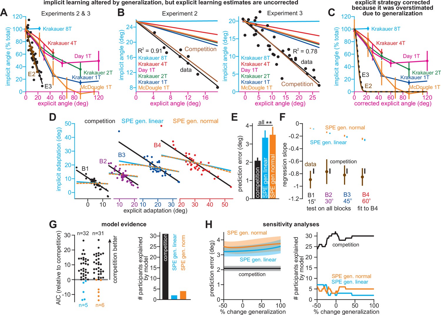
(A) Aim-centered generalization could create the illusion that implicit and explicit systems compete. To evaluate this possibility, we compared the implicit-explicit relationship in Exps. 2 and 3 to generalization curves reported in Krakauer et al., 2000, Day et al., 2016, and McDougle et al., 2017. The 1T, 2T, 4T, and 8T labels correspond to the number of adaptation targets in Krakauer et al. The gold McDougle et al. curve is particularly relevant because the authors controlled aiming direction on generalization trials and counterbalanced CW and CCW rotations. Data in Exps. 2 and 3 are shown overlaid in the inset. Implicit learning declined about 300% more rapidly with increases in re-aiming than that observed by Day et al. The solid black and brown lines show the competition theory predictions. Implicit learning in Experiments 2 and 3 was normalized to its theoretical maximum, reached when re-aiming is equal to zero. The value used to normalize was determined via linear regression (25.5° in Exp. 2, 19.7° in Exp. 3). (B) Same as in A, but without normalizing implicit learning. Generalization curves were converted to degrees by multiplying the curves in A by the max. implicit learning value in Exp. 2 (25.5°) or Exp. 3 (19.7°). (C) The comparisons in A and B are not correct. Under the generalization hypothesis, each data point’s explicit strategy needs to be corrected according to generalization. This inset shows the true implicit-explicit generalization curve that would be required to produce the data in A and B. The E2 and E3 lines show the Exp. 2 and Exp. 3 curves. (D) Points show implicit and explicit learning measured in the stepwise individual participants studied in Exp. 1 (B1 is 15° period, B2 is 30° period, B3 is 45° period, and B4 is 60° period). Three models were fit to participant data in the 60° period. Competition model fit is shown in black. A linear generalization (SPE gen. linear) with slope set by McDougle et al. is shown in cyan. A Gaussian generalization (SPE gen. normal) with width set by McDougle et al. is shown in gold. Since models were fit to B4 data, the B1, B2, and B3 lines represent predicted behavior. (E) The prediction error (RMSE) in each model’s implicit learning curve across the held-out 15°, 30°, and 45° periods in D. (F) Linear regressions fit to each rotation block in (D). Brown points and lines (data) show the regression slope and 95% CI. The black (competition), cyan (SPE gen. linear), and gold (SPE gen. normal) are model predictions where lines are 95% CIs estimated via bootstrapping. (G) All three models in D–F were fit to individual participant behavior in the stepwise group. At left, the AIC for each model is compared to that of the competition model. At right, the total number of subjects best captured by each model is shown. (H) Same as E and G but where the generalization width was varied in a sensitivity analysis. We tested values between one-half the McDougle et al. generalization curve (–50%) and twice the McDougle et al. generalization curve (+100%). Error bars in E show mean ± SEM. Statistics in E are post-hoc tests following one-way rm-ANOVA: **p < 0.01.
-
Figure 4—source code 1
Figure 4 data and analysis code.
- https://cdn.elifesciences.org/articles/65361/elife-65361-fig4-code1-v2.zip
Figure 4—figure supplement 1
Implicit variations are inconsistent with generalization.
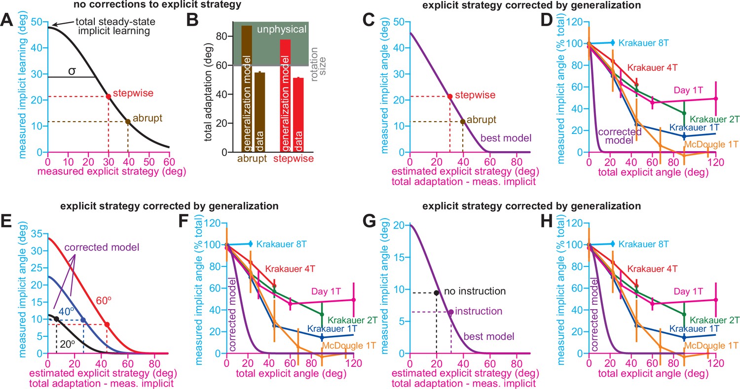
(A) We fit a Gaussian generalization curve to the implicit and explicit learning measures in the stepwise (red) and abrupt (brown) groups in Exp. 1. The curve’s peak indicates total steady-state implicit learning. For both stepwise and abrupt groups to have the same total implicit learning, this would require total implicit learning to equal 47.8° (total steady-state implicit learning in the graph) and a standard deviation equal to 23.6° (σ in the graph). (B) The analysis in A does not yield physiological results. Total adaptation would be calculated by adding the total steady-state implicit learning to the explicit strategy (x-axis in A). This would yield total learning equal to 87.3° and 77.7° in the abrupt and stepwise groups, respectively (bars labeled generalization model). Yet the rotation was only 60°: gray line (rotation size). Thus, total learning must exceed the rotation to yield the measurements in A. Total learning in both the stepwise and abrupt groups is also provided in the inset (bars labeled data). (C&D) The violation in A&B is that measured explicit strategy is estimated as total adaptation minus measured implicit learning. Explicit strategy estimate will greatly overestimate true explicit strategy. In these insets, we corrected this in the model. In (C), we show the model when implicit learning decrements due to generalization, and strategy is estimated as total adaptation minus generalized implicit learning (best model). In D, we show the true underlying generalization curve that produces the implicit-explicit measures in C. The curve is shown in the corrected model. Note that such a curve is physiologically inconsistent with previously measured implicit learning properties. In E and F, we conduct a similar analysis, but this time analyze the response to the 20°, 40°, and 60° no-instruction rotations in Neville and Cressman, 2018. (E) shows the model’s behavior when implicit and explicit learning are both biased by generalization. The three curves correspond to each rotation size (total implicit learning scales because it is equal to pir). In F, we show the true Gaussian generalization curve (corrected model) that is needed to produce the data in C. Last, in G and H, we analyzed the response to instruction in Neville and Cressman. These insets are analogous to C and D.
-
Figure 4—figure supplement 1—source code 1
Figure 4—figure supplement 1 data and analysis code.
- https://cdn.elifesciences.org/articles/65361/elife-65361-fig4-figsupp1-code1-v2.zip
Figure 4—figure supplement 2

Differences in generalization across visuomotor rotation tasks.
(A) Data collected by Day et al., 2016, reported in Figure 2 of the original manuscript (Figure 4 in current manuscript). Here, participants were exposed to a 45° rotation while reaching to a single target. On each trial they were asked to report their aiming direction, using a ring of visual landmarks. In the ‘target’ group, implicit aftereffects were measured at the trained target location. In the ‘aim’ group, implicit aftereffects were probed at a target location 30° away from the trained target, consistent with the direction of the most frequently reported aim. Here we show data from the first aftereffect cycle after the rotation period. (B) Similar to A except for data reported by McDougle et al., 2017; Figure 3A of their manuscript. Participants were also exposed to a 45° rotation while reaching to a single target. At the end of the experiment, participants were exposed to an aftereffect block where participants were told to move straight to the target without re-aiming. Here we take two relevant points from the generalization curve measured at the end of learning. The ‘target’ condition represents aftereffects probed at the training target. The ‘aim’ condition shows the aftereffect measured at 22.5° away from the primary target, which was the target closest to the mean reported explicit re-aiming strategy of 26.2°. (C) Data again from Day et al. The ‘probe’ implicit learning measure is the same as A. The ‘report’ condition shows the amount of implicit learning estimated by subtracting the reported explicit strategy from the reported reach angle on the last cycle of the rotation. (D) Similar to C, but for the intermittent reporting (IR-E) group reported by Maresch et al. (Figure 4b of their manuscript). In this group aim was only intermittently reported (four trials for every 80 normal adaptation trials). Thus, in most cases, participants only had to attend to a single target when reaching. The authors also used eight training targets (as opposed to one in A–C). The ‘probe’ condition corresponds to the total implicit learning measured at the end of adaptation by telling participants to reach without re-aiming. The ‘report’ condition corresponds to the total implicit learning estimated at the end of adaptation by subtracting the reported aim direction from the measured reach angle. (E) Here, we report implicit learning measured using the ‘probe’ and ‘report’ conditions in Experiment 2, analogous to the measures described in D. Error bars show mean ± SEM.
-
Figure 4—figure supplement 2—source code 1
Figure 4—figure supplement 2 data and analysis code.
- https://cdn.elifesciences.org/articles/65361/elife-65361-fig4-figsupp2-code1-v2.zip
Figure 5 with 4 supplements
Implicit-explicit correlations with total adaptation match the competition theory.
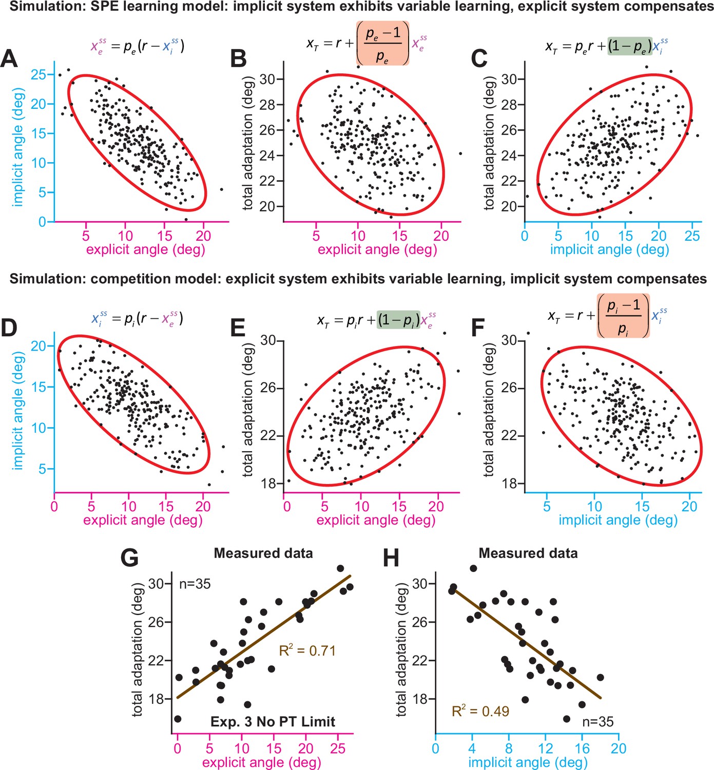
The competition equation states that xiss = pi(r – xess), where pi is a scalar learning gain depending on ai and bi. The competition between steady-state implicit (xiss) and explicit (xess) adaptation predicted by this model is simulated in D across 250 hypothetical participants. The model pi is fit to data in Experiment 3. Total learning is given by xTss = xiss + xess. These two equations can be used to derive expressions relating total learning (xTss) to steady-state implicit (xiss) and explicit (xess) learning. In E, we show that the competition theory predicts a positive relationship between explicit learning and total adaptation (equation at top derived in Appendix 7, green denotes a positive gain). In F, we show that the competition theory predicts a negative relationship between implicit learning and total adaptation (equation at top derived in Appendix 7, red shading denotes negative gain). In (A–C), we consider an alternative model. Suppose that implicit learning is immune to explicit strategy and varies independently across participants. This is equivalent to the SPE learning model. But in this case, the explicit system could respond to variability in implicit learning via another competition equation: xess = pe(r – xiss). Here, pe is an explicit learning gain (must be less than one to yield a stable system). In A, we show the negative relationship between implicit and explicit adaptation predicted by this alternate SPE learning model. In B, we show that when the explicit system responds to implicit variability (SPE learning) there is a negative relationship between total adaptation and explicit strategy. The equation at top is derived in Appendix 7. In C, we show that the SPE learning model will yield a positive relationship between implicit learning and total adaptation. Equation at top derived in Appendix 7. (G) We measured the relationship between explicit strategy and total adaptation in Exp. 3 (No PT Limit group). Total learning exhibits a positive correlation with explicit strategy. (H) Same concept as in G, but here we show the relationship between total learning and implicit adaptation. The patterns in G and H are consistent with the competition theory (compare with E and F).
-
Figure 5—source code 1
Figure 5 data and analysis code.
- https://cdn.elifesciences.org/articles/65361/elife-65361-fig5-code1-v2.zip
Figure 5—figure supplement 1
Relationships between implicit, explicit, and total learning indicate competition.
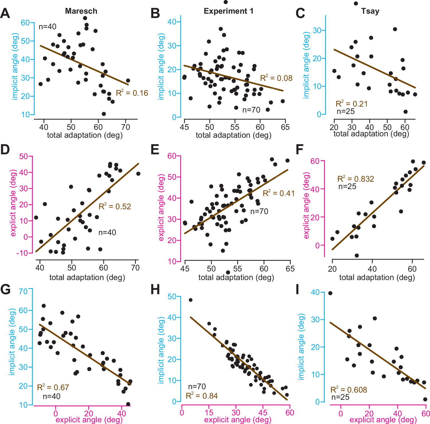
Data were analyzed across three experiments. In the left column, we report participants in the CR, IR-E, and IR-EI groups in Maresch et al., 2021 In the middle column, we report participants collapsed across the abrupt and stepwise 60° rotation period in Experiment 1. In the right column, we report participants in the 60° rotation group in Tsay et al., 2021a. In each experiment, we analyzed implicit learning, explicit learning, and total adaptation. Implicit and explicit learning were estimated with exclusion (‘no aiming’) trials. (A–C) The relationship between implicit learning and total adaptation. (D–F) The relationship between explicit learning and total adaptation. (G–I) Relationship between implicit and explicit learning. All lines in A–I denote a linear regression. The associated R2 statistic is shown in each inset. All relationships were statistically significant (p < 0.05). Dots in each inset denote individual participants.
-
Figure 5—figure supplement 1—source code 1
Figure 5—figure supplement 1 data and analysis code.
- https://cdn.elifesciences.org/articles/65361/elife-65361-fig5-figsupp1-code1-v2.zip
Figure 5—figure supplement 2
Factors that weaken the correlation between implicit learning and total adaptation.
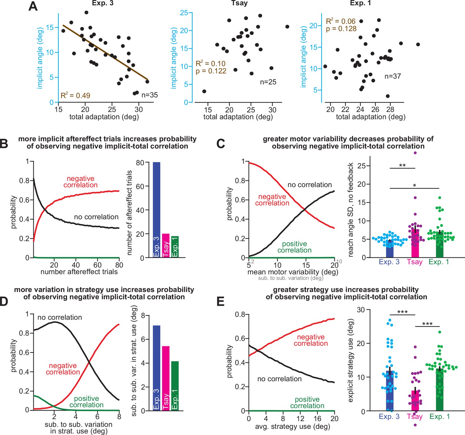
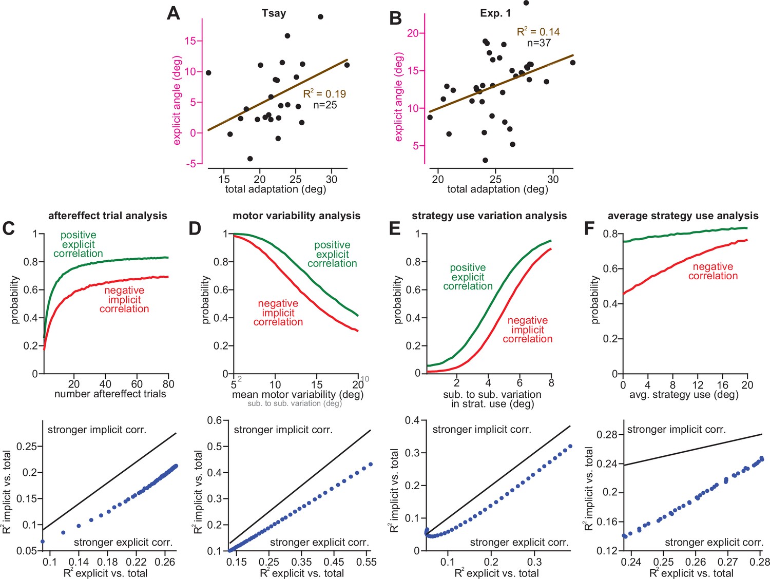
(A) At left, we reproduce the relationship between implicit learning and total adaptation in the No PT Limit group in Experiment 3. In the middle inset, the same analysis is shown for participants in the 30° group in Tsay et al., 2021a. At right, the same analysis is shown for participants in the stepwise 30° rotation period in Experiment 1. Relationships between implicit learning and total adaptation were not statistically significant (p > 0.05) at middle and right. In B–E we explore factors that can weaken the relationship between implicit learning and total adaptation in the competition theory. The four factors are: B, total number of aftereffect trials used to measure implicit learning, (C), motor variability in the reach, (D), between-subject variability in strategy use, and E, total strategy use in the subject population. At left in each inset we conducted a power analysis. In this power analysis, n = 30 participants were simulated. Explicit strategies were randomly sampled. Implicit learning was then obtained via the competition equation. Implicit, explicit, and total learning were calculated for each simulated participant, by averaging over a set number of trials. Simulations were repeated 40,000 times. The probability that a negative relationship (red line), positive relationship (green line), and no relationship (black line) occurred is shown in the left inset. In B, at left, we show that with fewer trials to measure implicit learning, the probability that an experiment will yield a statistically significant relationship between implicit learning and total adaptation decreases substantially. At right, we compare the total number of “no aiming” trials used to measure implicit learning in Exp. 3, Tsay et al., and Exp. 1 (stepwise). In C, at left, we show that increases in trial-to-trial reach variability (i.e. motor execution noise) dramatically reduce the probability than an experiment will produce a statistically significant relationship between implicit learning and total adaptation. At right, we analyze trial-to-trial variability during the no aiming period in each experiment. In D, at left, we show that little variability in strategy use across participants reduces the probability that an experiment will yield a negative relationship between implicit learning and total adaptation. At right, we show the standard deviation in explicit strategies across subjects in the three experiments. In (E), at left, we show that little overall strategy use in the subject population decreases the probability that an experiment will yield a negative relationship between implicit learning and total adaptation. At right, we compare explicit strategies across the three experiments. Statistics in C and E denote a one-way ANOVA.
-
Figure 5—figure supplement 2—source code 1
Figure 5—figure supplement 2 data and analysis code.
- https://cdn.elifesciences.org/articles/65361/elife-65361-fig5-figsupp2-code1-v2.zip
Figure 5—figure supplement 3
Correlations between explicit learning and total adaptation are more robust to between-subject implicit variability.
(A) Here, we show the correlation between explicit strategy and total adaptation in the 30° rotation group in Tsay et al., 2021a. (B) Same as A, but for the stepwise 30° rotation period in Experiment 1. In C–F, we show implicit and explicit correlations with total adaptation can be weakened by four factors: (C), total number of aftereffect trials used to measure implicit and explicit learning, (D), motor variability in the reach, (E), between-subject variability in strategy use, and (F), total strategy use in the subject population. At left in each inset we conducted a power analysis. In this power analysis, n = 30 participants were simulated. Explicit strategies were randomly sampled. Implicit learning was then obtained via the competition equation. Implicit, explicit, and total learning were calculated for each simulated participant, by averaging over a set number of trials. Simulations were repeated 40,000 times. At top we show the probability over these iterations that a statistically significant positive relationship between explicit strategy and total adaptation (green lines) and negative relationship between implicit learning and total adaptation (red lines) occur. At bottom, we calculated the average R2 value for the implicit-total and explicit-total regressions. Each point compares the two R2 values for each simulation condition above, with the unity line (black). In C, we show that more aftereffect trials improves the probability of obtaining statistically significant correlations, but the explicit-total correlation is stronger than the implicit-total correlation. In D, we show that less motor variability improves the probability of obtaining statistically significant correlations, but the explicit-total correlation is stronger than the implicit-total correlation. In E, we show that greater subject-to-subject variability in strategy improves the probability of obtaining statistically significant correlations, but the explicit-total correlation is stronger than the implicit-total correlation. In F, we show that greater overall strategy improves the probability of obtaining statistically significant correlations, but the explicit-total correlation is stronger than the implicit-total correlation.
-
Figure 5—figure supplement 3—source code 1
Figure 5—figure supplement 3 data and analysis code.
- https://cdn.elifesciences.org/articles/65361/elife-65361-fig5-figsupp3-code1-v2.zip
Figure 5—figure supplement 4
Variance in implicit learning properties weakens the relationship between implicit learning and total adaptation in the competition theory.
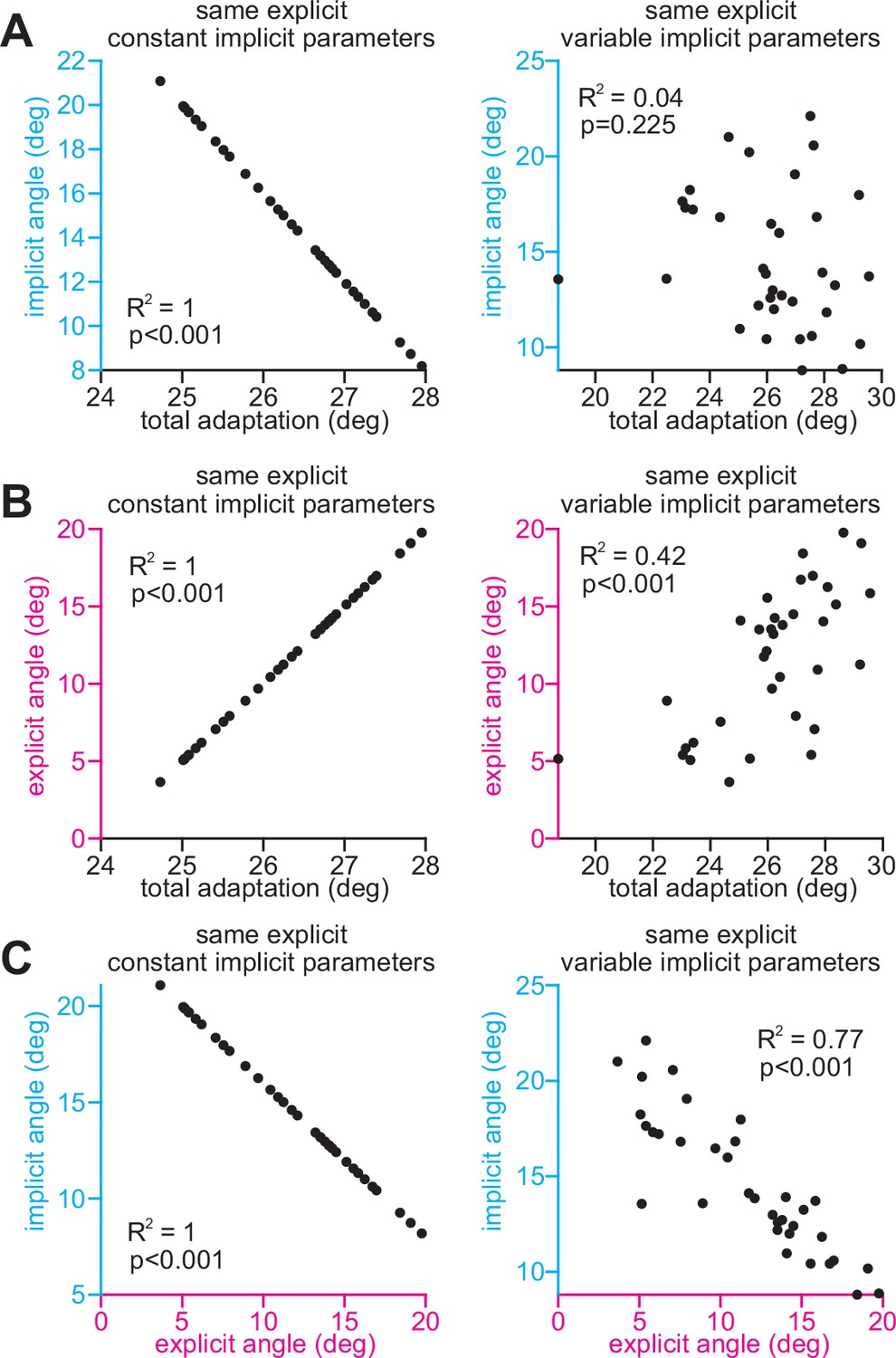
Here, we consider two sources of variability: (1) subject-to-subject variability in explicit strategy, and (2) subject-to-subject variability in implicit learning. We simulate explicit strategies across 35 participants. The explicit strategies are the same in the left column (same explicit) and the right column (same explicit). They are sampled from a normal distribution: mean = 12°, SD = 4°. However, the left and right columns differ in terms of implicit variability. In the left column, there is no implicit variability across subjects. Implicit learning was calculated using the competition theory, using the same implicit learning gain (pi = 0.8). In the right column, we added variability to this implicit learning gain. This represents the more realistic scenario, that implicit retention and error sensitivity vary across participants. The implicit learning gain was randomly sampled with a normal distribution, mean = 0.8, SD = 0.1. In A, we show the relationship between implicit learning and total adaptation in these toy cases. In B, we show the relationship between explicit learning and total adaptation in these toy cases. In C, we show the relationship between implicit learning and explicit learning in these toy cases. Note that the relationship between implicit learning and total adaptation (A, at right) was uniquely susceptible to variability (p = 0.225), whereas other correlations remained strong and statistically significant (B and C, at right).
-
Figure 5—figure supplement 4—source code 1
Figure 5—figure supplement 4 analysis code.
- https://cdn.elifesciences.org/articles/65361/elife-65361-fig5-figsupp4-code1-v2.zip
Figure 6
Competition predicts changes in implicit error sensitivity without changes in implicit learning rate.
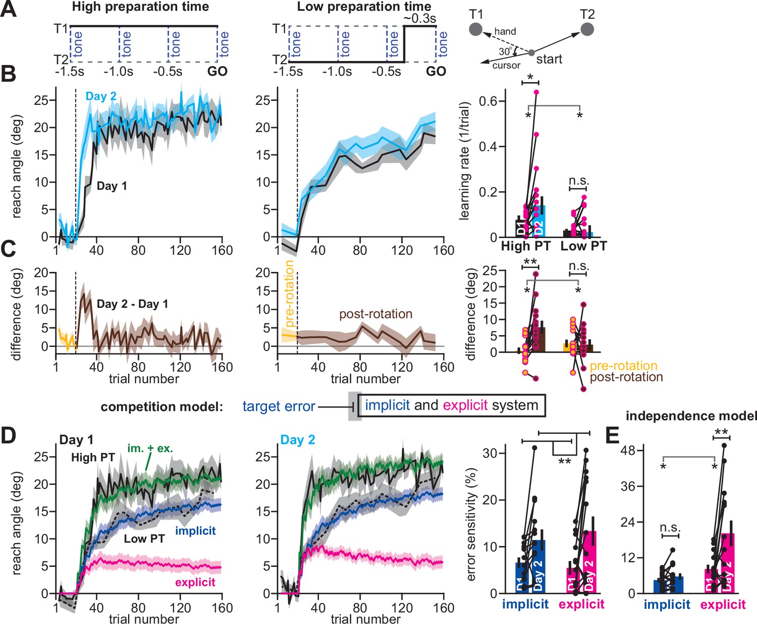
(A) Haith et al., 2015 instructed participants to reach to Targets T1 and T2 (right). Participants were exposed to a 30° visuomotor rotation at Target T1 only. Participants reached to the target coincident with a tone. Four tones were played with a 500ms inter-tone-interval. On most trials (80%) the same target was displayed during all four tones (left, High preparation time or High PT). On some trials (20%) the target switched approximately 300ms prior to the fourth tone (middle, Low preparation time or Low PT). (B) On Day 1, participants adapted to a 30° visuomotor rotation (Day 1, black) followed by a washout period. On Day 2, participants again experienced a 30° rotation (Day 2, blue). At left, we show the reach angle expressed on High PT trials during Days 1 and 2. Dashed vertical line shows perturbation onset. At middle, we show the same but for Low PT trials. At right, we show learning rate on High and Low PT trials, during each block. (C) As an alternative to the rate measure shown at right in B, we calculated the difference between reach angle on Days 1 and 2. At left and middle, we show the learning curve differences for High and Low PT trials, respectively. At right, we show difference in learning curves before and after the rotation. ‘Pre-rotation’ shows the average of Day 2 – Day 1 prior to rotation onset. ‘Post-rotation’ shows the average of Day 2 – Day 1 after rotation onset. (D) We fit a state-space model to the learning curves in Days 1 and 2 assuming that target errors drove implicit adaptation. Low PT trials captured the implicit system (blue). High PT trials captured the sum of implicit and explicit systems (green). Explicit trace (magenta) is the difference between the High and Low PT predictions. At right, we show error sensitivities predicted by the model. (E) Same as in D, but for a state-space model where implicit learning is driven by SPE, not target error. Model-predicted error sensitivities are shown. Error bars across all insets show mean ± SEM, except for the learning rate in B which displays the median. Two-way repeated-measures ANOVA were used in B, C, D, and E. For B and C, exposure number and preparation time condition were main effects. For D and E exposure number and learning system (implicit vs explicit) were main effects. Significant interactions in B, C, and E prompted follow-up one-way repeated-measures ANOVA (to test simple main effects). Statistical bars where two sets of asterisks appear (at left and right) indicate interactions. Statistical bars with one centered set show main effects or simple main effects. Statistics: n.s. means p > 0.05, *p < 0.05, **p < 0.01.
-
Figure 6—source code 1
Figure 6 data and analysis code.
- https://cdn.elifesciences.org/articles/65361/elife-65361-fig6-code1-v2.zip
Figure 7
Changes in implicit adaptation depend on both implicit and explicit error sensitivity.
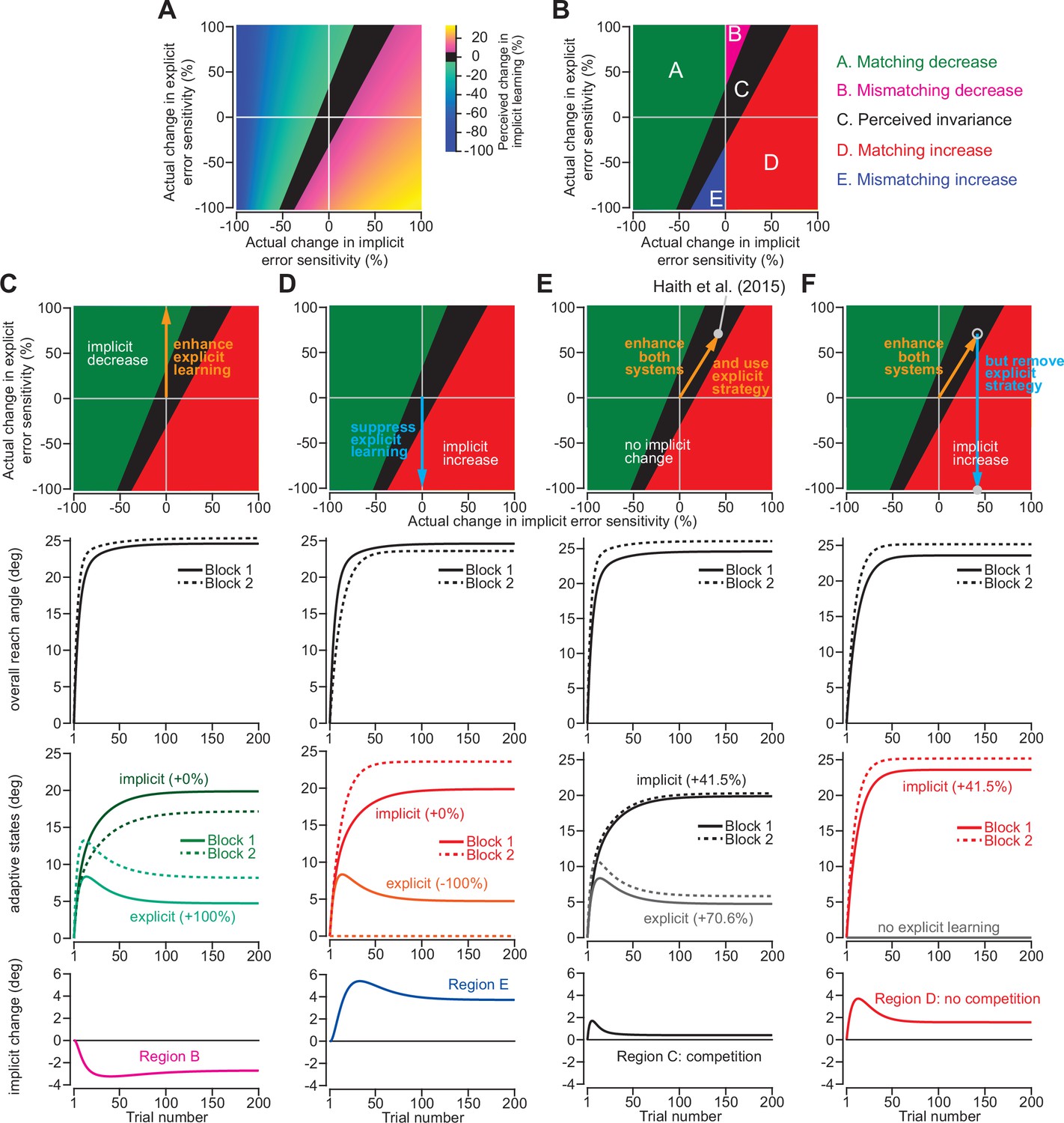
(A) Here we depict the competition map. The x-axis shows change in implicit error sensitivity between reference and test conditions. The y-axis shows change in explicit error sensitivity. Colors indicate the percent change in implicit adaptation (measured at steady-state) from the reference to test conditions. Black region denotes an absolute change less than 5%. The map was constructed with Equation 8. (B) The map can be described in terms of five different regions. In Region A (matching increase), implicit error sensitivity and total implicit adaption both increase in test condition. Region D is same, but for decreases in error sensitivity and total adaptation. In Region B (mismatching decrease), implicit learning decreases though its error sensitivity is higher or same. In Region E (mismatching increase), implicit learning increases though its error sensitivity is lower or same. Region C shows a perceived invariance where implicit adaptation changes less than 5%. (C) Row 1: effect of enhancing explicit learning. Row 2: total learning increases. Row 3: implicit and explicit learning shown in Blocks 1 and 2, where only difference is 100% increase in explicit error sensitivity. Row 4: change in implicit learning (Block 2–1). (D) Row 1: effect of suppressing explicit learning. Row 2: total learning decreases. Row 3: implicit and explicit learning shown in Blocks 1 and 2, where explicit error sensitivity decreases 100%. Row 4: implicit learning change (Block 2–1). (E) Row 1: model simulation for Haith et al., 2015. Row 2: Total learning increases. Row 3: implicit and explicit learning during Blocks 1 and 2 where implicit error sensitivity increases by 41.5% and explicit error sensitivity increases by 70.6%. Row 4: negligible change in implicit learning (Block 2–1). (F) Same as in E except here explicit strategy is suppressed during Blocks 1 and 2.
-
Figure 7—source code 1
Figure 7 analysis code.
- https://cdn.elifesciences.org/articles/65361/elife-65361-fig7-code1-v2.zip
Figure 8 with 1 supplement
Removing explicit strategy reveals savings in implicit adaptation.
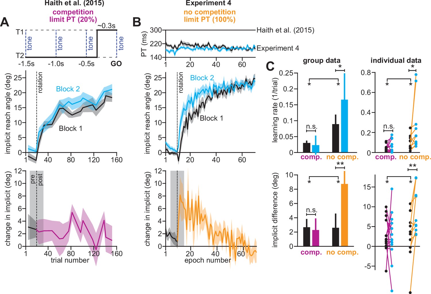
(A) Top: Low preparation time (Low PT) trials in Haith et al., 2015 used to isolate implicit learning. Middle: learning during Low PT in Blocks 1 and 2. Bottom: difference in Low PT learning between Blocks 1 and 2. (B) Similar to A, but here (Experiment 4) explicit learning was suppressed on every trial, as opposed to only 20% of trials. To suppress explicit strategy, we restricted reaction time on every trial. The reaction time during Blocks 1 and 2 is shown at top. At middle, we show how participants adapted to the rotation under constrained reaction time. At bottom, we show the difference between the learning curves in Blocks 1 and 2. These two periods were separated by washout cycles with veridical feedback (not shown). (C) Here, we measured savings in Haith et al. (20% of trials had reaction time limit) and Experiment 3 (100% of trials had reaction time limit). Top row: we quantify savings by fitting an exponential curve to each learning curve. Data are the rate parameter associated with the exponential. Left column shows group-level data (median). Right column shows individual participants. Bottom row: we quantify savings by comparing how Blocks 1 and 2 differed before perturbation onset (black), and after perturbation onset (purple and yellow). At left, error bars show mean ± SEM. At right, individual participants are shown. Error bars in A and B indicate mean ± SEM. Statistics in C show mixed-ANOVA (exposure number is within-subject factor, experiment type is between-subject factor). Significant interactions were observed both in rate (top) and angular (bottom) savings measure. Follow-up simple main effects were assessed via one-way repeated-measures ANOVA. Statistical bars where two sets of asterisks appear (at left and right) indicate interactions. Statistical bars with a centered set show simple main effects. Statistics: n.s. means p > 0.05, *p < 0.05, **p < 0.01.
-
Figure 8—source code 1
Figure 8 data and analysis code.
- https://cdn.elifesciences.org/articles/65361/elife-65361-fig8-code1-v2.zip
Figure 8—figure supplement 1

Limiting preparation time eliminates explicit strategy use.
(A) Participants were exposed to a 30° rotation. The perturbation schedule is shown at top. The reach angle on each cycle is shown in the middle. The preparation time on each cycle is shown at bottom. On each trial, we imposed a strict upper limit on reaction time in an attempt to suppress explicit strategy. Participants were separated into two groups. These groups had an identical perturbation schedule but received different instructions prior to the terminal no feedback period. In the Limit PT group (n = 21, red), participants were instructed to aim directly at the target without re-aiming. In the decay-only group (n = 12, black), participants were instructed to imagine the rotation was still present, and to continue trying to move the “imagined cursor” through the target. Change in reach angle in the Limit PT no feedback condition could be due to abandoning explicit strategy and also decay in a temporally-labile implicit process (instruction period was about 30 s in duration). Change in reach angle in the decay-only no feedback condition was intended to isolate any decay in a temporally-labile implicit process. (B) Change in reach angle due to instruction. Here, we subtracted the initial reach angle during the no feedback period from the total adaptation measured prior to instruction. We observed no statistically significant difference between the two groups (two-sample t-test) suggesting that change in reach angle during the no feedback period was almost entirely due to involuntary decay in a temporally-labile implicit process. Error bars indicate mean ± SEM.
-
Figure 8—figure supplement 1—source code 1
Figure 8—figure supplement 1 data and analysis code.
- https://cdn.elifesciences.org/articles/65361/elife-65361-fig8-figsupp1-code1-v2.zip
Figure 9

Removing explicit strategy reveals anterograde interference in implicit adaptation.
(A) Top: participants were adapted to a 30° rotation (A). Following a 5-min break, participants were then exposed to a –30° rotation (B). This A-B paradigm was similar to that of Lerner et al., 2020 Middle: to isolate implicit adaptation, we imposed strict reaction time constraints on every trial. Under these constraints, reaction time (blue) was reduced by approximately 50% over that observed in the self-paced condition (green) studied by Lerner et al., 2020. Bottom: learning curves during A and B in Experiment 5; under reaction time constraints, the interference paradigm produced a strong impairment in the rate of implicit adaptation. To compare learning during A and B, B period learning was reflected across y-axis. Furthermore, the curves were temporally aligned such that an exponential fit to the A period and exponential fit to the B period intersected when the reach angle crossed 0°. This alignment visually highlights differences in the learning rate during the A and B periods. (B) Here, we show the same analysis as in A but when exposures A and B were separated by 24 hr. (C) To measure the amount of anterograde interference on the implicit learning system, we fit an exponential to the A and B period behavior. Here, we show the B period exponential rate parameter divided by the A period rate parameter (values less than one indicate a slowing of adaptation). At left, group-level statistics are shown. At right, individual participants are shown. Data in the Limit PT (limited preparation time) condition in Experiment 5 are shown in blue. Data from Lerner & Albert et al. (no preparation time limit) are shown in green. A two-way ANOVA was used to test for differences in interference (preparation time condition (i.e. experiment type) was one between-subject factor, time-elapsed between exposures (5 min vs 24 hr) was the other between-subject factor). Statistical bars indicate each main effect. Statistics: *p < 0.05, **p < 0.01. Error bars in each inset show mean ± SEM.
-
Figure 9—source code 1
Figure 9 data and analysis code.
- https://cdn.elifesciences.org/articles/65361/elife-65361-fig9-code1-v2.zip
Figure 10
Two visual targets create two implicit error sources.
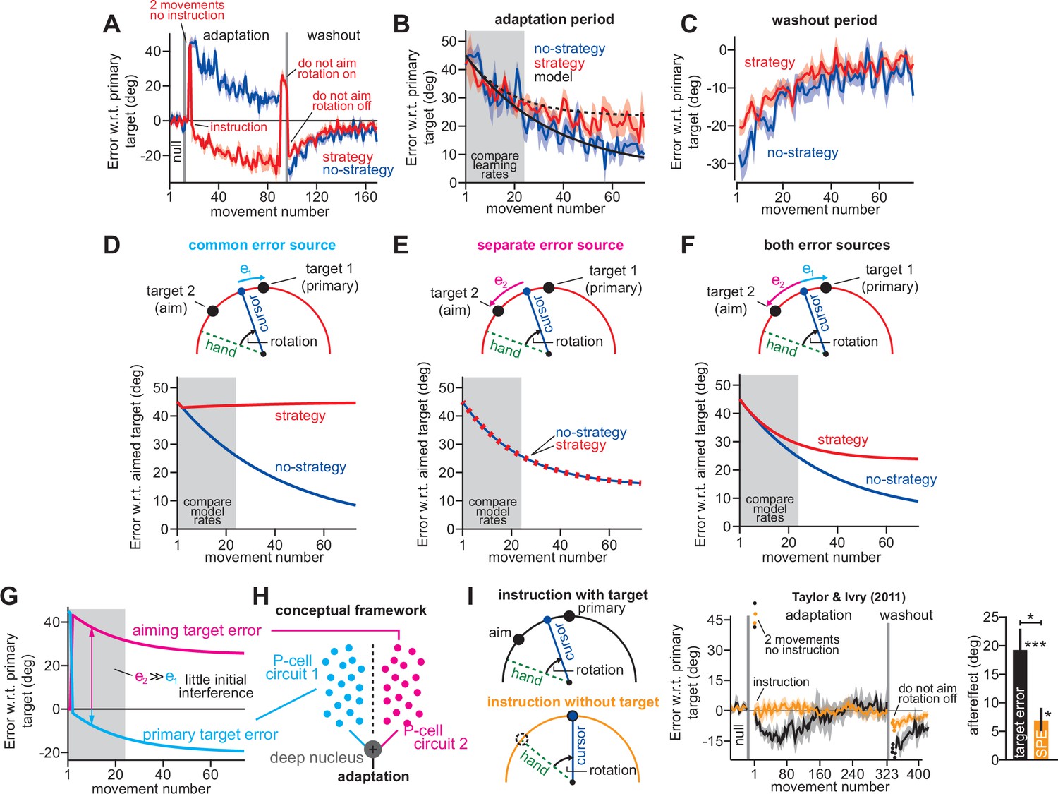
(A) Data reported in Mazzoni and Krakauer, 2006. Blue shows error between primary target and cursor during adaptation and washout. Red shows the same, but in a strategy group that was instructed to aim to a neighboring target (instruction) to eliminate target errors, once participants experienced two large errors (two cycles no instruction). (B) The error between the cursor and the aimed target during the adaptation period. These curves are the same as in A except we use the aimed target rather than primary target, so as to better compare learning curves across groups. (C) The washout period reported in A. Here, error is relative to primary target, though in this case aimed and primary targets are the same. (D) We modeled behavior when implicit learning adapts to primary target errors e1. Note that the no-strategy learning group resembles data. However, strategy learning exhibits no drift because the implicit system has zero error. Note here that the primary target error of 0° is a 45° aimed target error in the strategy group. (E) Similar to D, except here the implicit system adapts to errors between the cursor and aimed target, termed e2. (F) In this model, the strategy group adapts to both the primary target error and the aimed target error (e1 and e2 at top). The no-strategy group adapts only to the primary target error. Learning parameters are identical across groups. (G) We show how aiming target and primary target errors evolve in the strategy group in F. (H) A potential neural substrate for implicit learning. The primary target error and aiming target error engage two different sub-populations of Purkinje cells in the cerebellar cortex. These two implicit learning modules combine at the deep nucleus. (I) Data reported in Taylor and Ivry, 2011. Before adaptation, subjects were taught to re-aim their reach angles. In the ‘nstruction with target’ group, participants re-aimed during adaptation with the aid of neighboring aiming targets (top-left). In the ‘instruction without target’ group, participants re-aimed during adaptation without any aiming targets, solely based on the remembered instruction from the baseline period. The middle shows learning curves. In both groups, the first two movements were uninstructed, resulting in large errors (two movements no instruction). Note in the ‘instruction with target’ group, there is an implicit drift as in A, but participants eventually reverse this by changing explicit strategy. There is no drift in the ‘instruction without target’ group. At right, we show the implicit aftereffect measured by telling participants not to aim (first no feedback, no aiming cycle post-adaptation). Greater implicit adaptation resulted from physical target. Error bars show mean ± SEM. Statistics: *p < 0.05, ***p < 0.001.
-
Figure 10—source code 1
Figure 10 data and analysis code.
- https://cdn.elifesciences.org/articles/65361/elife-65361-fig10-code1-v2.zip
Author response image 1
Measuring the aftereffect on the last 10 washout trials in Mazzoni and Krakauer, 2006.
Author response image 2
Here we split the data in Experiments 1-3 into low and high strategy groups (based on the median strategy).
We fit a regression to the ‘low-strategy’ group (blue line) and the ‘high-strategy’ group (magenta line). We compared the slope and intercept to see if there was a systematic difference in the regression’s gain and bias for low and high strategy cases.
Author response image 3

Model fits to Saijo and Gomi (2010).
Author response image 4
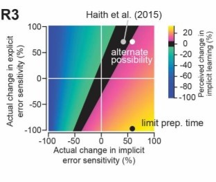
Shows the hypothetical scenario described by Reviewer 3.
Additional files
Download links
A two-part list of links to download the article, or parts of the article, in various formats.
Downloads (link to download the article as PDF)
Open citations (links to open the citations from this article in various online reference manager services)
Cite this article (links to download the citations from this article in formats compatible with various reference manager tools)
Competition between parallel sensorimotor learning systems
eLife 11:e65361.
https://doi.org/10.7554/eLife.65361


