Organ geometry channels reproductive cell fate in the Arabidopsis ovule primordium
- DIADE, University of Montpellier, CIRAD, IRD, France
- Department of Plant and Microbial Biology and Zurich-Basel Plant Science Center, University of Zürich, Switzerland
- Laboratoire Reproduction et Développement des Plantes, University of Lyon, ENS Lyon, UCB Lyon 1, CNRS, INRAE, INRIA, France
Figures
Figure 1 with 1 supplement
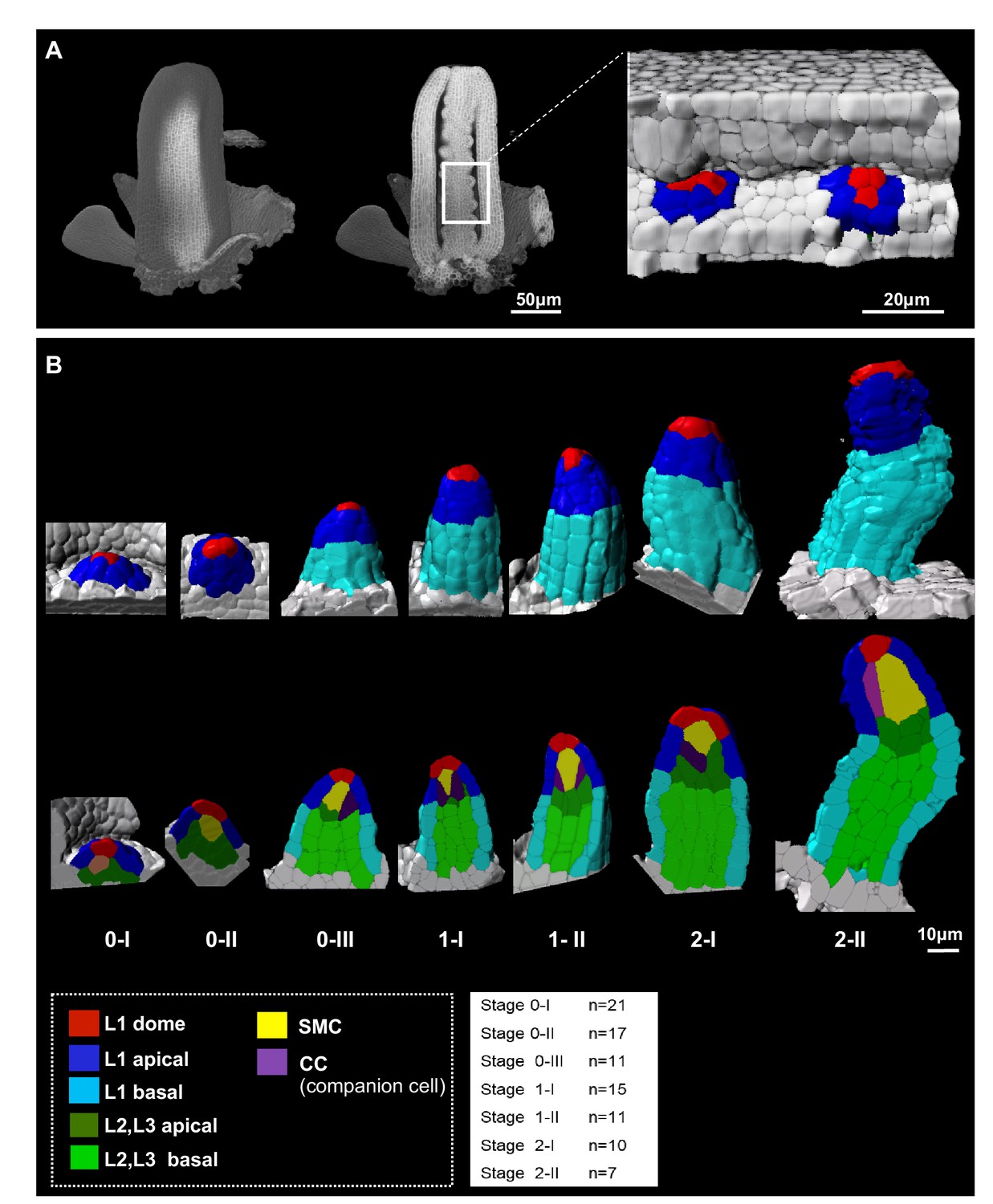
Reference set of 3D segmented images capturing Arabidopsis ovule primordium growth at cellular resolution.
(A) 3D reconstruction of a whole gynoecium stained with PS-PI (cell wall dye) and visualized by CSLM. The cross-section shows nascent ovule primordia attached to the placenta. (B) Ovule primordium developmental stages (0-I to 2-II) and organ viewpoints (domains) defined for 3D quantitative analyses. All segmented data can be analyzed by an interactive interface named OvuleViz. See also Figure 1—figure supplement 1A–C. n = number of ovules analyzed. Segmented images for all developmental stages are provided in Figure 1—source data 1. See also Figure 1—figure supplement 1D–E, Materials and methods.
-
Figure 1—source data 1
Image gallery.
- https://cdn.elifesciences.org/articles/66031/elife-66031-fig1-data1-v2.pdf
Figure 1—figure supplement 1
Approaches for morphodynamic analyses of ovule primordium development using a reference set of 3D segmented images.
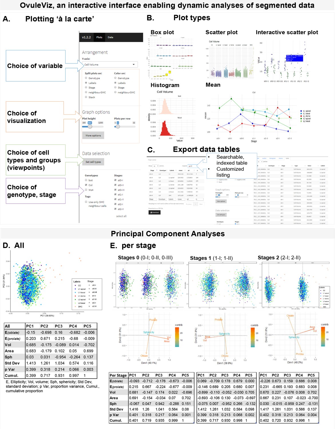
(A) OvuleViz, an interactive interface enabling the analysis of segmented data based on exported cell statistics. The different snapshots display several features of OvuleViz, enabling the generation of plots from chosen cell statistics for chosen ovule primordium stage, genotype, cell labels or groups thereof (viewpoints). (B) Examples of plot types that can be generated by OvuleViz. (C) Possibility to export all or a subset of data as summary table or raw dataframe for further analyses external to OvuleViz. (D) PCA of cell descriptors from the wild-type reference dataset (Arabidopsis Col-0) (see Figure 1—source data 1), for all cell types and all stages. PCA was performed on a dataset containing Sphericity, Ellipticity oblate, Ellipticity prolate, Area, and Volume. Only the first and the second Principal Components (PCs) are shown. The loading plot and table indicate the variables’ contribution to each component. (E) Same as (D) for all cell types grouped by stage: stage 0 (0-I; 0-II), stage 1 (1-I; 1-II), and stage 2 (2-I; 2-II). Variables’ contributions are presented by loading plots for each PC and summary table.
Figure 2 with 2 supplements
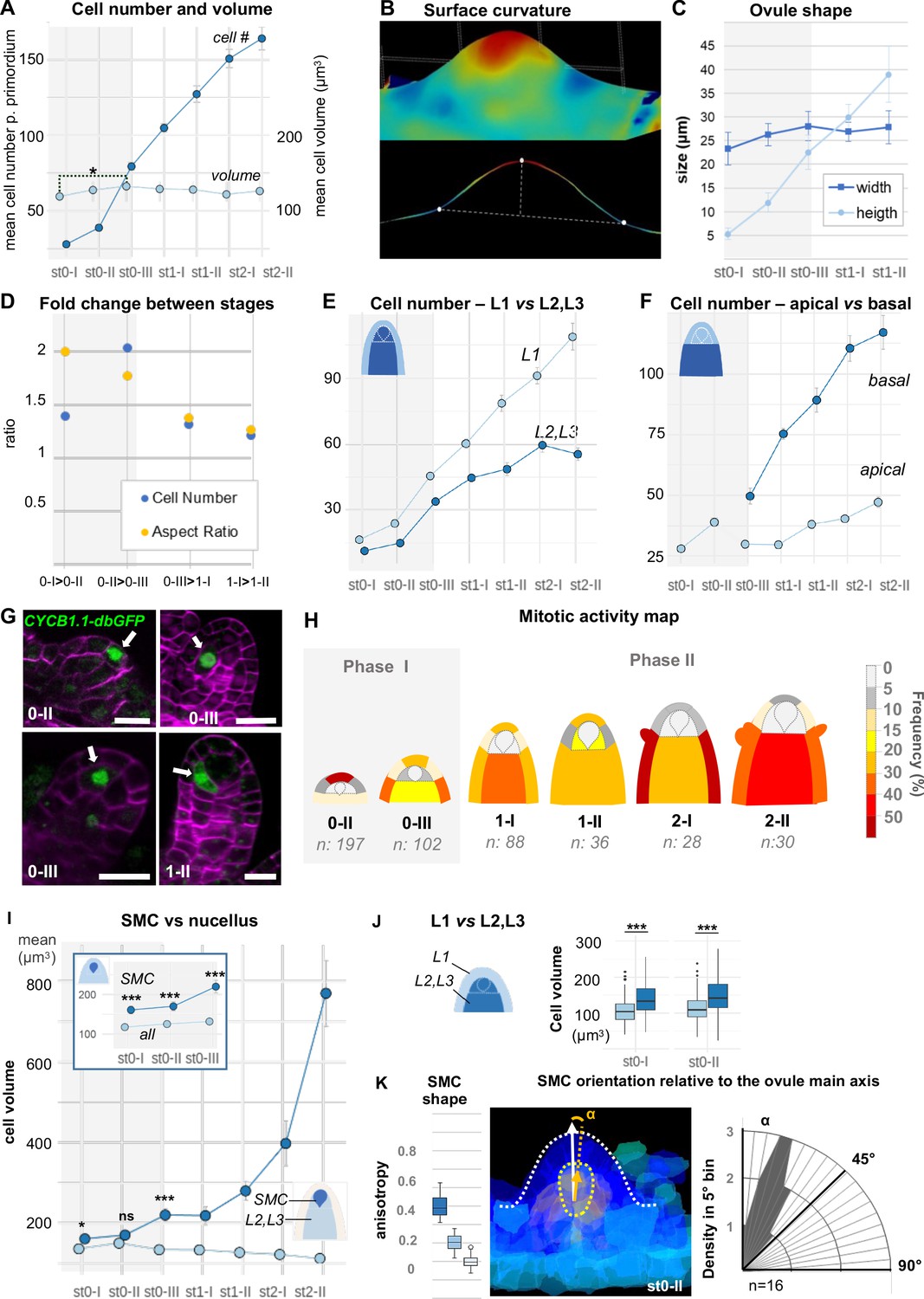
Ovule primordium morphogenesis involves domain-specific cell division and anisotropic cell growth.
(A) Mean cell number per ovule increases mainly during stages 0-I to 0-III (Phase I), whereas cell volume per ovule remains constant on average across primordium development (stages 0-I to 2-II). (B) Representative image of a continuous surface of an ovule primordium mesh and its projected median plane. Dashed lines indicate the minimal and maximal curvature points used to measure organ height and width. Color scale: minimal curvature mm-1 (see also Figure 2—figure supplement 1B). (C) Anisotropic organ growth during Phase I and until stage 1-II. Mean width and height were quantified per stage. (D) Phase I shows distinct growth dynamics compared to Phase II. Fold-change of cell number and aspect ratio between stages are plotted. (E) Mean cell number is increased at the L1 vs. L2,L3 layers across developmental stages. (F) Mean cell number is increased in the basal vs. apical domain across developmental stages. (G) Representative images of ovule primordia expressing the M-phase reporter promCYCB1.1::CYCB1.1db-GFP (CYCB1.1db-GFP). White arrows indicate dividing cells. Magenta signal: Renaissance SR2200 cell-wall label. Scale bar: 10 µm. (H) Domain-specific map of mitotic activity during ovule primordium development, scored using the CYCB1.1db-GFP reporter. The frequency of mitoses was calculated per ovule domain at each developmental stage and color-coded as indicated in the bar (right). n: total number of scored ovules. (I) Mean SMC candidate volume (dark blue) is significantly increased as compared to L2,L3 cells (pale blue) from stage 0-III onward, on even at earlier stages as compared to all other cells (inset). (J) Mean cell volume is increased in L2,L3 cells as compared to L1 cells, at the two early developmental stages (0-I, 0-II). (K) The SMC consistently displays anisotropic shape with main axis of elongation aligned with ovule growth axis. The SMC anisotropy index (boxplot, left; stage 0-II, n = 16 ovules) was calculated from the Maximum (dark blue), Minimum (light blue), and Medium (medium blue) covariance matrix eigenvalues, computed from 3D segmented cells (see Figure 2—figure supplement 1G). Image (middle): illustration of the SMC main anisotropy axis (orange arrow) related by an angle ‘alpha’ to the main axis of the ovule primordium (white arrow), stage 0-II. Radar plot (right): ‘alpha’ angle measured on z projections for n = 16 ovule primordia at stage 0-II. See also Materials and methods. Error bars: Standard errors to the mean. Differences between cell types or primordium domains were assessed using a two-tailed Man Whitney U test in (A) and (I); a two-tailed Wilcoxon signed rank test in (J). *p≤0.05, **p≤0.01, ***p≤0.001. See also Figure 2—figure supplement 1, Figure 2—source data 1, Materials and methods.
-
Figure 2—source data 1
Raw data for quantitative analysis.
- https://cdn.elifesciences.org/articles/66031/elife-66031-fig2-data1-v2.xlsx
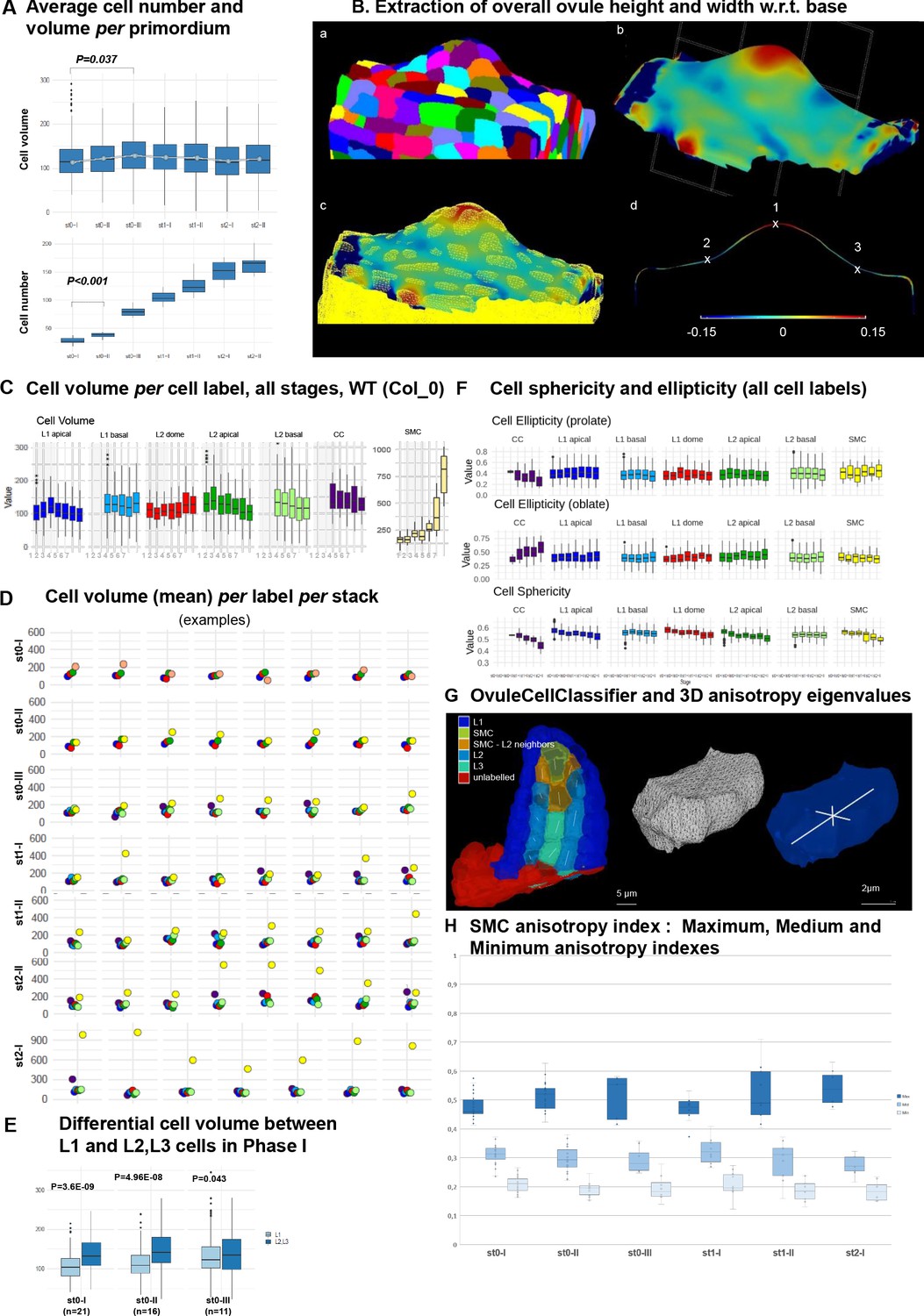
Figure 2—figure supplement 1
Ovule primordium morphogenesis involves domain-specific cell division and anisotropic cell growth patterns.
(A) Average cell number and cell volume in wild-type (Col) ovule primordium during development. Mann Whitney U test was used to assess the difference of each stage relative to the previous stage. Related to Figure 2A. (B) Extraction of overall ovule height and width used in Figure 2B,C. (a) Segmented stack imported in MorphoGraphX, (b) continuous surface mesh created in MorphoGraphX with the minimal curvature projected, the clipping plane is shown (dashed grid), (c) comparison between cell-mesh and continuous mesh, (d) longitudinal section of the mesh showing maximal (1) and minimal (2 and 3) curvature points. Heatmap: minimal curvature mm−1. Related to Figure 2B–C. (C) Box plots and line plot (error bar is standard error of the mean) showing the mean cell volume in each ovule domain during all developmental time points. Mann Whitney U test was used to assess the difference between stages (L1 apical). Related to Figure 2I. (D) Scatter plots comparing the cell volume of SMC (yellow) to the average cell volume of other cells types (same color code as in Figure 1) per ovule primordium, per stage. Related to Figure 2I. The color code follows that of the cell label in panel C. (E) Comparison of cell volume between L1 and L2L3 cells in Phase I ovule primordia (stages 0-I to 0-III). Wilcoxon Signed Rank test was used to assess the difference between domains. Related to Figure 2J. (F) Quantification of cell sphericity and ellipticity (prolate and oblate, see Materials and methods) at all ovule primordium domains during development. (G) Computation of covariance matrix eigenvalues for cell anisotropy analysis: Left: semi-automated cell type classification showing labeled cells along a longitudinal cut of an ovule. L2 SMC neighbors (orange) stands for all L2 cells sharing a portion of their wall with the SMC (yellow). Unlabeled cells (red) are not considered in the analysis. For the inner cells, the main anisotropy axis (the eigenvector of the covariance matrix corresponding to the biggest eigenvalue) is shown with a white line. Right: representation of eigenvectors of the covariance matrix (white lines) used for the PCA analysis on cell anisotropy on a random cell. The eigenvectors are scaled by their own eigenvalue normalized over the sum of the three eigenvalues. The longest eigenvector is aligned with the longest cell axis, the shortest with the shortest cell axis and the mid eigenvector with the cell axis orthogonal to the other two (and of intermediate length). Related to Figure 2K. See also movie in Figure 2—video 1 and Appendix 1. (H) SMC anisotropy index calculated from Maximal (dark blue), Mid (mid blue) and Minimal (pale blue) eigenvalues, normalized by the sum of all, from stage 0-I to stage 2-I. Related to Figure 2K. p values: *p≤0.05, **p≤0.01, ***p≤0.001. See also Figure 2—source data 1.
Figure 2—video 1
Semi-automated cell-type classification and anisotropy quantification with MorphoMechanX.
Figure 3 with 3 supplements
Mechanical and cell-based 2D simulation models of ovule primordium development predict that ovule shape depends on cell growth anisotropy.
(A–B) Schematic representation of the main parameters as described in Table 2 used for the reference model and variation models shown in C and Figure 3—figure supplement 1. The L1 and underlying L2,L3 layers are represented, arrows of different size indicate anisotropy, the bulged dotted lines represent the ability of the tissue to (passively) grow under strain, the gray fields represent the initial domain of the growth signal (pale gray) and the domain of fixed, high concentration (dark gray square), *, for FEM-simulations only. Deviations of these parameters are shown in red. (C–D) Tissue-based FEM simulations of ovule primordium growth. (C) Growth stability is reached at T = 24 in the reference FEM Model 1. (D) Simulations omitting the anisotropic growth parameter (FEM-Model 3) show abnormal ovule dome shape at the same simulation time. The magnitude of accumulated strain is indicated by the background color (according to the heatmap), while the principal strain directions are shown as fine lines (white: positive strain, corresponding to stretch, red: negative strain, corresponding to compression). (E–H) Cell-based MS simulations of ovule primordium growth showing growth signal distribution and anisotropy index at the indicated simulation times (T). (E) Reference Model (MS-Model 2) showing a realistic primordium shape with straight flanks, sharp curvature at the apex, and a narrow base at T = 190. (G) The reference model shows the emergence of a large, anisotropic cell with trapezoidal shape in the L2 at T = 58, confirmed at T = 132. (F) Simulation with isotropic cell growth in inner L2,L3 layers (MS-Model 3) produces a primordium with enlarged apex and basis and flatter dome at the same simulation time as in the Reference Model. (H) L2 cells in MS-Model 3 show reduced anisotropy as compared to the Reference Model. See also Figure 3—figure supplement 1, Table 2, Appendix 1 for modeling hypotheses and methods.
Figure 3—figure supplement 1
FEM- and MS-based simulations, reference models, and additional variations.
(A) Time series of the FEM reference simulation: FEM-Model 1 and its preparation. Left: reference simulation progression; the lines represent the in-plane principal strains: white for extensive, red for compressive. The heatmap represents the trace of the Green-Lagrange strain tensor. Tables (middle): preparation of the reference template (a–c) and initial parameters (d). (a–c) the starting template is a flat tissue representation distinguishing L1 and inner layers on which anisotropic material (a, Young’s modulus E2), material stiffness (b, Young’s modulus E1E3), and the growth signal (c, Kpar) domain are set. The white lines in the images left indicate the direction of fiber reinforcement for the anisotropic material (a), the intensity of the stiffness in the isotropic component of the material (b), the direction of signal-based growth, which is orthogonal to the fiber reinforcement direction (c). In addition, all lateral boundaries of the simulation template (except the top one) were fixed in all degrees of freedom. The table (d) integrates the visual information with global parameters. See additional explanations in the Materials and Methods. Schematic representation (right) of the main parameters modulated in the models shown in B and compared to the reference model for the L1 and underlying (L2,L3) layers. Arrows of different size indicate anisotropy, the bulged dotted line represent the ability of the tissue to (passively) grow under strain, the gray fields represent the initial domain distribution of the growth signal (pale gray) and the domain of fixed, high concentration (dark gray square). Deviations of these parameters are shown in red in the panel B. (B) Variation of the signal-based growth distribution with respect to the FEM- and MS-based reference models. For all model variations, the result is shown for the continuous FEM-based simulations (top) and the MS-based simulations (middle) at the simulation time point indicated (T), a schematic representation of the altered parameter is shown in red following the scheme template in A (bottom). color scale: same as in panels A and D for FEM- and MS-models, respectively. (a) Model 4: the signal is allowed to diffuse broadly. In both FEM- and MS-based simulations, the primordium is broader and the flanks are not orthogonal to the surface (arrow) as in the reference models. (b) Models 5: L1-driven growth hypothesis (1). Here, the growth-specifying signal is set at a high and fixed (i.e. non-diffusing) concentration only in the L1. In both simulations, these conditions allow the formation of a protrusion but not a realistic primordium. For both simulations, the growth time went beyond the reference time to reach the same final height as in the reference models and to compensate for the prescribed reduced growth intensity. Specific observations are made for the different simulations: FEM-Model 5 shows high compression forces below the L1 (arrow: compressive areas are marked by the blue color and red lines). One interpretation is that these compressions may arise because the L1 ‘collapses’ toward the center in the absence of inner tissue growth. Note the narrower apical, subepidermal domain than in the reference model. Furthermore, in the periclinal direction the L1 experiences significant compressions (indicated by the red lines). MS-Model 5: the growth is not balanced and generated an unstable apex (arrow, winding in different directions during growth, see Figure 3—video 1). (c) Models 6: L1-driven growth hypothesis (2). Here, the growth signal is restricted solely to the L1. In this case, the difference is striking for both FEM- and MS-based simulations: the models are not able to create a significant buckle and, even if strain-based growth is permitted, the inner tissue is not pulled upwards. The growing part of the L1 ends being compressed by the non-growing counterpart (as shown by the compressive strain marked in blue in the image for the FEM-based simulation), causing the simulation to numerically fail earlier than the reference (FEM) or in any case not forming a primordium (MS). (d) Models 7: exclusive inner-tissue growth hypothesis. Here, the growth signal is absent in the L1. The L1 performs exclusively passive strain-based relaxation. In this model, we test whether it is plausible that growth can be entirely initiated by the inner tissues, provided the L1 has a higher ability to relax (compared to the remaining tissue) due to induced strain. In such a scenario, the inner layer, which is prescribed to grow as in the reference model, pushes the L1, causing accumulation of tensile strains in the periclinal direction that get released due to passive strain-based relaxation. Both FEM- and MS-based simulations are able to produce a digit-shaped protrusion, even if, in the FEM-based simulation, it is shorter with less straight flanks (i.e. smoother transition from the placenta to the flanks; dotted arrow). This can be explained by the absence of compressive strains at the base of the ovule (plain arrow) in comparison with the reference model. The MS-based model displays a primordium with increased width at the apex. A possible explanation for this may be the absence of growth constraints generated by the L1. In both cases, the passive strain-based relaxation coefficient of the L1 was higher than in the reference model. Whether this is biologically relevant remains to be addressed experimentally. (C) Models varying passive strain-based relaxation and material properties. Results are shown for the continuous FEM-based simulations (top) and the MS-based simulations (bottom) at the simulation time point indicated (T). (a) Models 8: absence of passive strain-based relaxation in all the tissue. In both simulations, this results in a poorly developed primordium (and numerically the simulation fail earlier than the reference time), likely due to the accumulation of high strains (and stresses), particularly visible in the FEM-based model (high accumulation of compressive and tensile strains near each other in the inner tissue as well as in the L1, arrows). (b) Model 8a: variation of the previous model with absence of passive strain-based relaxation only in the L1. In both simulations, the primordium is shorter than in the reference case, although less severe in the FEM-based simulation. Specifically, in the L1 there is a high accumulation of tensile stresses on the outer walls in the apical portion and in the inner walls at the base (arrows). (c) FEM-Model 2: absence of anisotropic material properties in all tissues. Although the simulation produced a well-shaped primordium, the L1 is slightly thicker (double sided arrow, 1.2-fold compared to reference Model 1) and there is a larger L2,L3 apical domain characterized by a principal strain oriented 90° to that in the reference model (insets). These morphological differences with the reference model can be explained by the fact that passive strain-based relaxation in an isotropic material has an equal effect in the periclinal and the anticlinal direction, producing a thicker L1 and a rounder dome. In (d) FEM-based Model 2b: variation of previous Model 2. Here, only the L1 has anisotropic material properties. This restores the L1 thickness control but the abnormally high intensity and modified direction of compressive strains are similar to that in Model 2. (D) Mass spring reference model and initial template preparation, comparison with data from real ovules. Top left: MS-Model 2 simulation at four different time points. The heatmap indicates the intensity of the growth-specifying signal. Bottom left: reference simulation performed on a template obtained from a real ovule placenta (see also Materials and Methods). Top right: Initial parameters at simulation start. Field values as indicated (a–g) used to set up the reference configuration shown on the placenta at simulation time 0 and MS global parameters (h). More details can be found in the Materials and Methods. Bottom right: comparison between simulation and real primordia. Image: 3D, segmented ovule primordia stage 0-II from the wild-type reference set (see main text), longitudinal view: the SMC (orange) is outlined in a white triangular mesh (color-code refers to cell volume). Its morphology is to be compared to SMC candidates produced in the reference Model MS-Model 2 (e.g. T = 134 for grid-based simulation and T = 108 for real-image template-based simulation): the cell is elongated, centrally located in the apical dome and presents a broader upper periclinal wall surface compared to the bottom one. Plot: comparison of height-width ratio along simulation progression in MS-Model 2 and developmental progression in real (from segmented images of the wild-type reference set, see main text). For the simulation, two equi-distanced time-points between the first (T = 0) and the last simulation time step (T = 190) have been used to compute the values for intermediate phases. (E) Variation of MS-Model 3 - Higher target area in central, L2 apical cell (MS-Model 3a). This model is based on the same hypotheses as in MS-Model 3. The only difference being that the central L2 cell, which in the other models has a target area of 100 um2 , has now a bigger target area prior to division (200 um2). The aim was to test whether longer cell growth influences anisotropy. The heatmap code represents the anisotropy index as defined in Appendix 1 and is scaled up to 1.2, hence with a narrower range than in Figure 3, to allow to appreciate the mild anisotropy level in the candidate SMC (index 1.18, a fully isotropic cell has index equal to 1, the fact that surrounding cells reach the maximum anisotropy index on this limited scale is not informative here). Furthermore, one can qualitatively appreciate that the cell shape is rather trapezoidal. This shows that if the SMC candidate grows longer than neighbouring cells, tissue geometrical constraints can confer cell anisotropy and a trapezoidal shape even in the context of isotropic specified growth, to reach a certain amount of anisotropy. (F) Model lacking cell growth anisotropy specifically in the L1 layer (MS-Model 3b). Strong alterations of ovule dome growth and shape were observed when isotropic cell growth was assigned exclusively to the L1 layer (complementary to growth anisotropy hypothesis in MS-Model 3). The ovule overall shape alterations are likely due to the fact that the same amount of signal-based growth has to be redistributed in the anticlinal and periclinal direction, limiting, though, the amount by which cells are prescribed to elongate. This, in turn, has a constraining effect on the inner layers. By comparing MS-Model 7 (B), where the L1 performs exclusively strain-based growth and MS-Model 3b, where selectively the L1 grows isotropically, it is possible to infer that the anticlinal component of growth in the L1 actively constraints the inner layer expansion. This constriction, in turn, causes a lack of tension build up at the interface between the L1 and L2 which limits then further periclinal strain-based growth in the L1, producing an ovule with a shorter dome and narrower apical domain. (G) Model intervening on SMC division. In the reference MS-Model 2, there is no explicit rule preventing division of the SMC candidate. To analyze the consequence of SMC growth on primordium growth in our models, we prevented the SMC candidate to divide at simulation time T = 110. Under the reference conditions where the turgor pressure is the same among all subepidermal cells, this generates a gigantic cell exerting a considerable tensile stretch on the surrounding cells, deforming the whole domain. This suggests that, in real ovules, SMC growth might be compensated by a reduction in turgor pressure, a hypothesis that needs to be tested. Note that the two direct adjacent cells have an elongated shape reminiscent of companion cells.
Figure 3—video 1
Mass Spring Model 2 (reference model) compared against Mass Spring Model 5 (epidermal driven growth).
Figure 3—video 2
Mass Spring Model 2 (reference model) compared against Mass Spring Model 3 (isotropic growth).
Figure 4 with 2 supplements
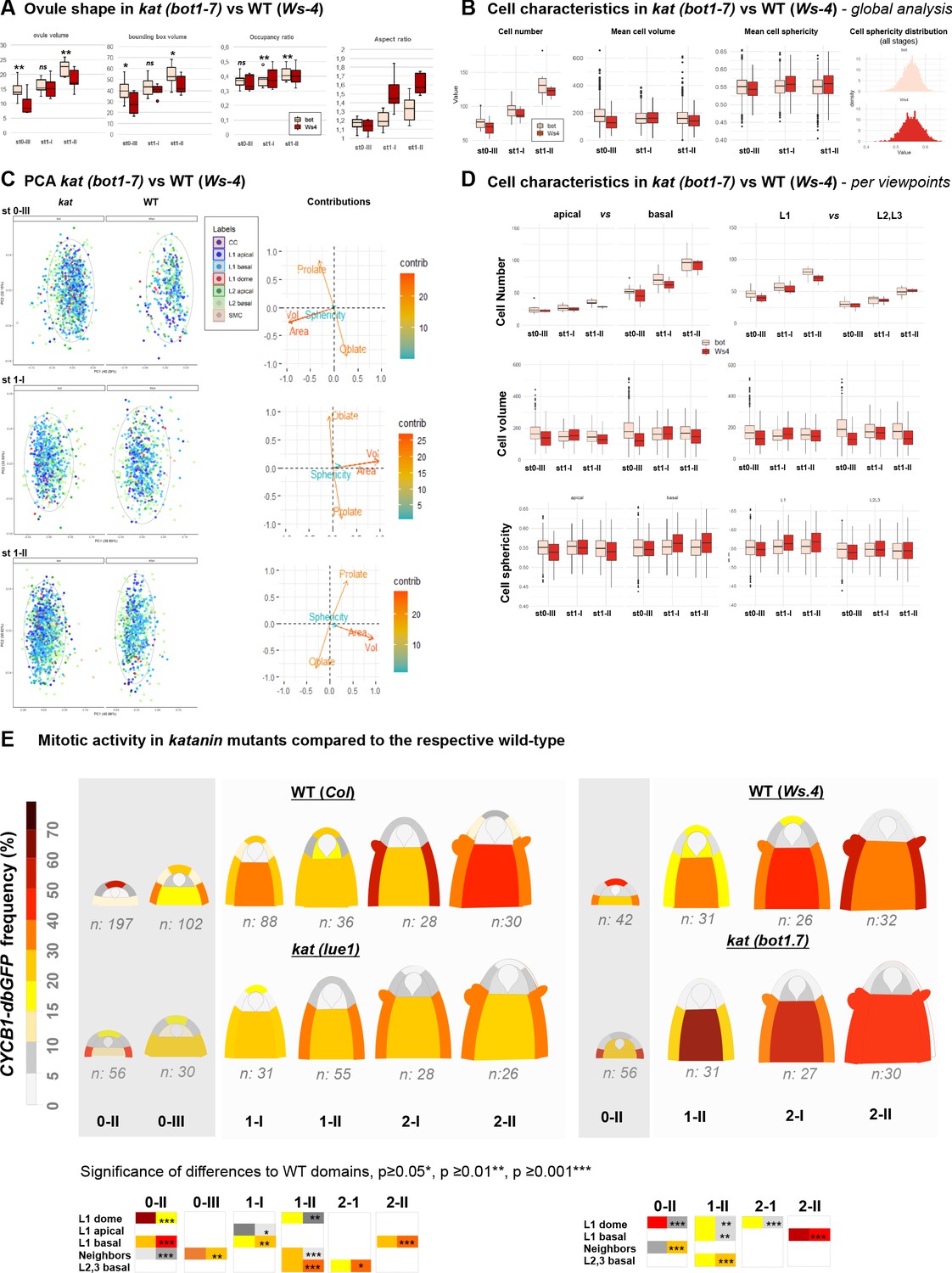
katanin mutants show a distinct ovule primordium geometry.
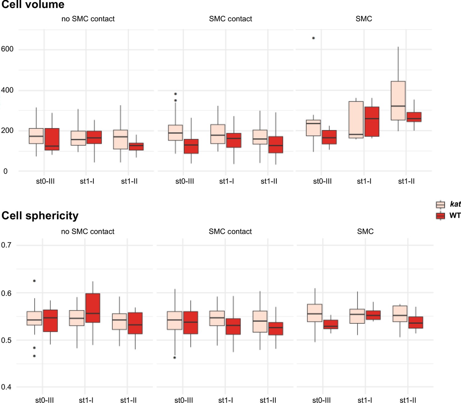
Comparison between wild-type (WT, Ws-4 accession) and katanin (kat, bot1-7 allele) ovule primordia. (A) 3D segmented images at stage 1-II. External organ view (top) and longitudinal sections (bottom) are shown. Scale bar 10 µm. See Figure 4—source data 1 for full datasets. (B–D) Morphological difference between WT and kat primordia measured by their volume (B), the aspect ratio (C), and aspect ratio to bounding box occupancy relationship (D). (D), Left: scheme representing the bounding box capturing the primordium’s 3D surface. See also Figure 4—figure supplement 2A. (E) Quantification of cell number, cell volume, and sphericity in comparisons of L1 vs. L2,L3 and apical vs. basal domains at stage 0-III. See also Figure 4—figure supplement 2C. (F) Mitotic activity domains are altered in kat primordia. Top: Heatmap of Log2 fold change of mitotic activity in the kat mutant (lue1 allele) vs. WT (Col-0) per domain, at two developmental stages. The frequency of mitoses was measured as in Figure 2. Full maps of mitotic activity in different mutant alleles are shown in Figure 4—figure supplement 2E. Bottom: representative images of kat primordia (lue1 allele) expressing CYCB1.1db-GFP. Dashed lines mark L2 apical cells. Magenta signal: Renaissance SR2200 cell wall label. Scale bar 10 µm. (G) Mean cell volume and sphericity are increased in kat L2 apical cells in contact with the SMC. SMC, cells in contact with the SMC, and cells not in direct contact with the SMC, are compared at stage 0-III. Color code in all plots: Dark red: WT; Salmon: kat mutant. Error bars: standard error of the mean. Differences between WT and kat mutants in (B), (C), (E), and (G) were assessed using a Mann Whitney U test; a two-tailed Fischer’s exact test was used in (F). p values: *p≤0.05, **p≤0.01, ***p≤0.001. See also Figure 4—figure supplements 1 and 2; and Figure 4—source data 2.
-
Figure 4—source data 1
Image gallery.
- https://cdn.elifesciences.org/articles/66031/elife-66031-fig4-data1-v2.pdf
-
Figure 4—source data 2
Raw data for quantitative analysis.
- https://cdn.elifesciences.org/articles/66031/elife-66031-fig4-data2-v2.xlsx
Figure 4—figure supplement 1
KATANIN localization pattern in ovule primordium.
(A) Localization of GFP:KTN1 (complementing ktn1-2 null mutant background), in the L1 outer wall of ovule primordium, detected by Airyscan super-resolution microscopy. KATANIN protein is detected as small foci frequently aligned with cellulose fibers. Insets are close up of the sectors outlined with white square on the image. GFP channel is displayed in green (two first ovules from the left), or in green and as heatmap (FIRE scale) of fluorescence intensity (third ovule at right). Cell wall cellulose fibers were stained with Renaissance SR2200 (grayscale signal). Scale bars: 10 µm. (B) Localization of GFP:KTN1 in median longitudinal section passing through the SMC (left) or adjacent section passing through the frontal SMC wall (SMC wall plane, right). SMC wall was located thanks to the cellulose dye Renaissance SR2200 (grayscale signal). Ovule primordia at stages 0 (top), 1 (middle) or 2 (bottom) were observed. KATANIN protein is detected more frequently in the L1 layer as indicated by relative fluorescence intensity heatmap visualization (FIRE scale). However, KATANIN signal is present also in internal layers, and notably in the SMC (white arrows) and its neighbors’ cells (yellow arrows). n: number of ovules observed (from nine independent plants). Scale bars: 10 µm.
Figure 4—figure supplement 2
katanin ovule growth defects.
(A) Ovule size, aspect ratio, bounding box, and bounding box occupancy. Ovule volume was calculated as the sum of cell volumes for individual ovules (OvuleViz data). For each ovule, the volume of their fitting bounding box (represented Figure 4D) was calculated using box side lengths given in Imaris (Bitplane, AG) on ovule primordia treated as Surface objects (see Materials and methods). Bounding box occupancy was calculated as the ratio of the ovule volume relative to its bounding box volume. The aspect ratio was calculated as the height (C length of the bounding box) divided by the mean of the width and depth lengths (A and B lengths of the bounding box). Man Whitney U test was used to assess differences between genotypes. Related to Figure 4B–D. (B) Comparison of cell number, cell volume, and sphericity in wild-type (WT) (Ws-4) and katanin (kat) ovule primordia (bot1-7 allele). Man Whitney U test was used to assess the differences between genotypes. (C) Global PCA analyses of cell characteristics in kat vs. WT ovules (Ws-4). PCA was performed on a dataset containing Sphericity, Ellipticity oblate, Ellipticity prolate, Area, and Volume measurements of WT and kat cells from ovules at the indicated stages (0-III, 1-I, 1-II). Cell types are labeled according to color code indicated. 95% confidence ellipses are indicated (dashed lines). Only the first and the second Principal Components (PCs) are shown. The loading plots indicate the contributions of the variables to each component. Related to Figure 4E. (D) Comparison of mean cell number, volume and sphericity in apical vs. basal domains, and in L1 versus L2,L3 layers between WT (Ws-4) and kat (bot1-7) ovule primordia. Man Whitney U test was used to assess differences between genotypes. Related to Figure 4E. (E) Mitotic activity in distinct domains of the ovule primordium of WT (Col, Ws-4) and kat (lue1, bot1.7) mutant plants. WT Col data are presented also in Figure 2 and shown here for better comparison only. The frequency of mitoses was scored using the CYCB1.1db-GFP reporter. Dark gray regions mark Phase I developmental stages. Two-tailed Fischer’s exact test was used to assess differences between domains in the genotypes. Significant p values (*p≤0.05, **p≤0.01, ***p≤0.001) are indicated for the different domains in colored boxes below the heatmaps (first column: WT; second column: kat). Non-significant differences are not represented. See also Figure 2—source data 1 and Figure 4—source data 1. Related to Figure 4F.
Figure 5 with 2 supplements
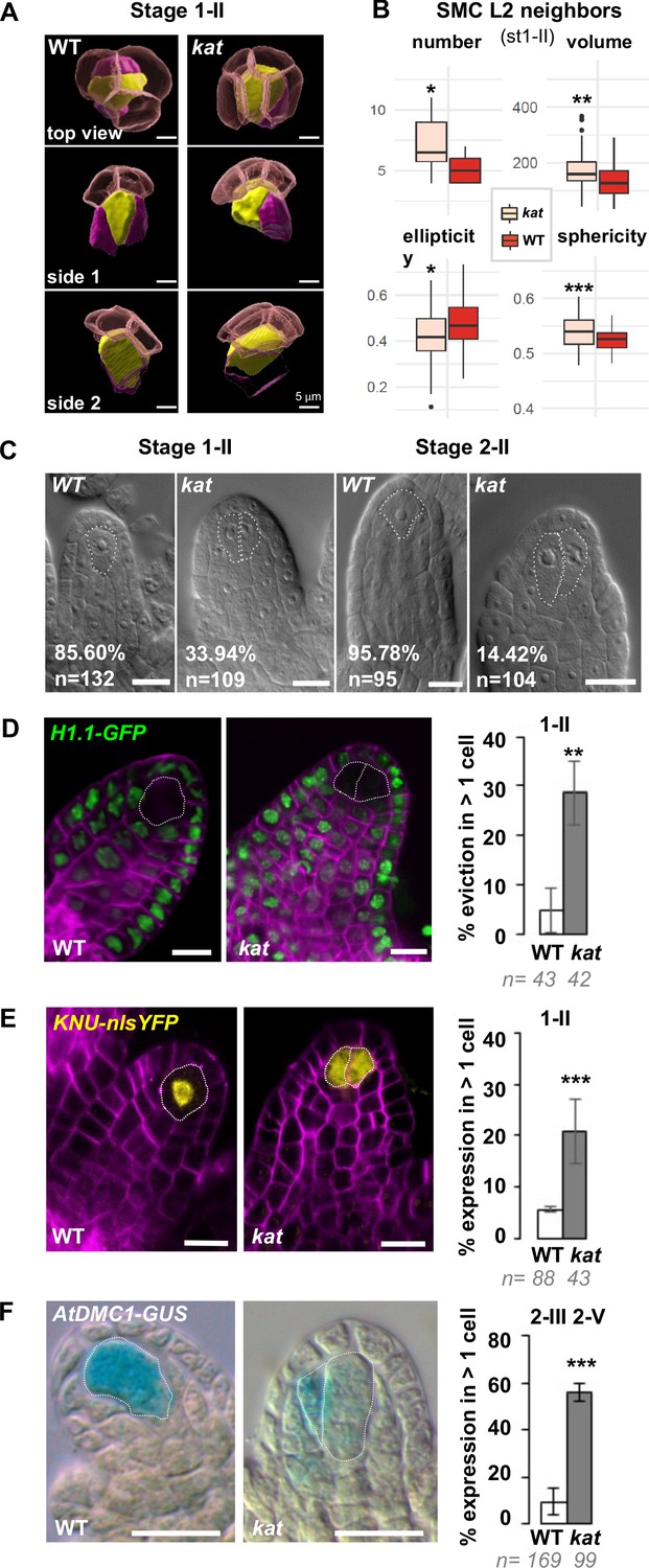
Altered ovule primordium geometry in katanin mutants is associated with multiple SMCs.
(A) SMCs lose their typical pear shape in kat mutants. 3D images of the apical-most cells in top and side view as indicated, showing the SMC (yellow), SMC neighbors (purple), and the L1 dome (transparent red). (B) Differential properties of L2,L3 apical domain cells (SMC and SMC neighbors) in terms of cell number, mean cell volume, ellipticity, and sphericity at stage 1-II. See also Figure 5—figure supplement 1 and Figure 4—source data 2. (C) Representative images of cleared wild-type (WT) and kat ovule primordia. The % indicate the frequency of ovules showing one SMC for WT primordia, or multiple SMC candidates (dashed lines) for kat primordia. (D–E) Representative images and quantification of SMC fate markers in WT and kat primordia: eviction of the H1.1::H1.1-GFP marker (green, D) and ectopic expression of KNU::nls-YFP (yellow, E) in more than one cell per primordia, are increased in kat primordia. See also Figure 5—figure supplement 2A. (F) The meiotic marker AtDMC1::GUS is ectopically expressed in kat ovules. Mutant alleles: bot1-7 (A–B), mad5 (C–E), lue1 (F). Additional kat alleles, stages, markers, and detailed quantifications are presented Figure 5—figure supplement 2 and Figure 5—source data 1. Magenta signal in (B) and (C): Renaissance SR2200 cell wall label. Scale bars for (A): 5 µm; for (C), (D), (E), (F): 10 µm. n: number of ovules scored. Error bar: standard error of the mean. Differences between WT and kat genotypes were assessed using a Mann Whitney U test in (B), and a two-tailed Fischer’s exact test in (C), (D), (E), and (F). p values: *p≤0.05, **p≤0.01, ***p≤0.001. See also Figure 5—figure supplements 1 and 2 and Figure 5—source data 1.
-
Figure 5—source data 1
Raw data for quantitative analysis.
- https://cdn.elifesciences.org/articles/66031/elife-66031-fig5-data1-v2.xlsx
Figure 5—figure supplement 1
Cell volume and sphericity of SMC and SMC neighbors in katanin.
Comparison of volume and sphericity of L2,L3 apical domain cells in wild-type (WT, Ws-4) and katanin (kat, bot1.7 allele). Mann Whitney U test was used to assess the differences between genotypes for the mean cell volume and sphericity visualized by boxplots. Related to Figure 5B.
Figure 5—figure supplement 2
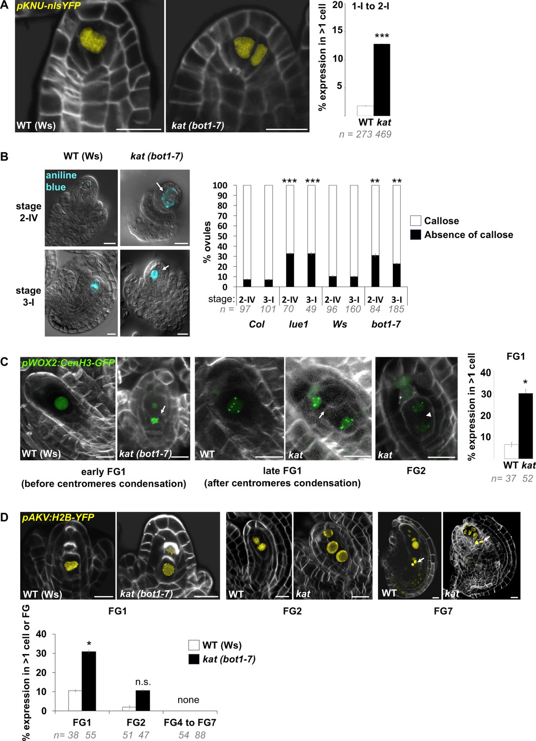
SMC and female gametophyte identity markers in katanin.
(A) Representative images and quantification of WT (Ws-4) and kat (bot1-7) ovule primordia expressing pKNU::nls-YFP (yellow signal), specifically expressed in the SMC. kat ovules show ectopic subepidermal cells with YFP signal, confirming SMC fate acquisition. Related to Figure 5E. (B) Representative images of WT (Ws-4) and kat (bot1-7) ovule primordia stained with aniline blue callose dye, and visualized with DIC and epifluorescence microscopy. Callose accumulates specifically in the SMC prior to meiosis (stage 2-IV) and in spore walls of a single tetrad (stage 3-I). In all ovules with callose-positive cells (blue signal), staining was observed in a single cell or tetrad, in both wild-type and katanin background. Representative kat ovules with ectopic enlarged cells which do not display callose are shown (white arrows). Quantification of the proportion of ovules at stages 2-IV and 3-I displaying or lacking callose accumulation, in WT (Col or Ws-4) and kat (lue1 or bot1-7), suggesting altered callose deposition in kat SMC. Related to Figure 5F. (C) Representative images (ca 10 um maximum intensity projections of image stacks) and quantification of WT (Ws-4) and kat (bot1-7) ovule primordia expressing pWOX2:CenH3-GFP (green signal), labeling centromeres from the functional megaspore stage (FG1) onward. Cells ectopically expressing the marker are detected in kat at both early (before centromeres condensation – left panel) and late (after centromeres condensation – middle panel) stages of functional megaspore formation. Ectopic spores were scored based on the presence of a cell wall (white arrows) separating the spores, by contrast to two-nuclei gametophyte stage (right image, shown as an example) where the two nuclei are separated by a vacuole (arrow head). Note that ectopic spores are aligned with the normal, most basal (chalazal) FM, suggesting that they belong to the same tetrad. They also display a similar number of centromeres (5) visible on the projections. Quantification was performed on pooled early and late FG1 stages. Related to Figure 5D–F. (D) Representative images and quantification of WT (Ws-4) and kat (bot1-7) ovule primordia expressing pAKV:H2B-GFP (yellow signal), labeling nucleus from the functional megaspore stage (FG1) to the mature female gametophyte stage (FG7). Spores ectopically expressing the marker are detected in kat at significant levels at FG1 stage (left panel and graph below), and non-significantly at stage FG2 (middle panel and graph below). From stage FG4 to stage FG7, katanin embryo sacs are often abnormal, however conspicuous expression of pAKV:H2B-GFP notably in antipodals cells (arrows, right panel) marked always a single embryo sac in kat ovules (noted as ‘none’ ectopic FG in the graph below). Related to Figure 5D–F. White signal: Renaissance SR2200 cell wall label. Scale bar: 10 µm. n: number of ovules scored. Error bar: standard error of the mean. Two-tailed Fischer’s exact test was used to assess differences between genotypes. p values: *p≤0.05, **p≤0.01, ***p≤0.001. See also Figure 5—source data 1.
Figure 6 with 1 supplement
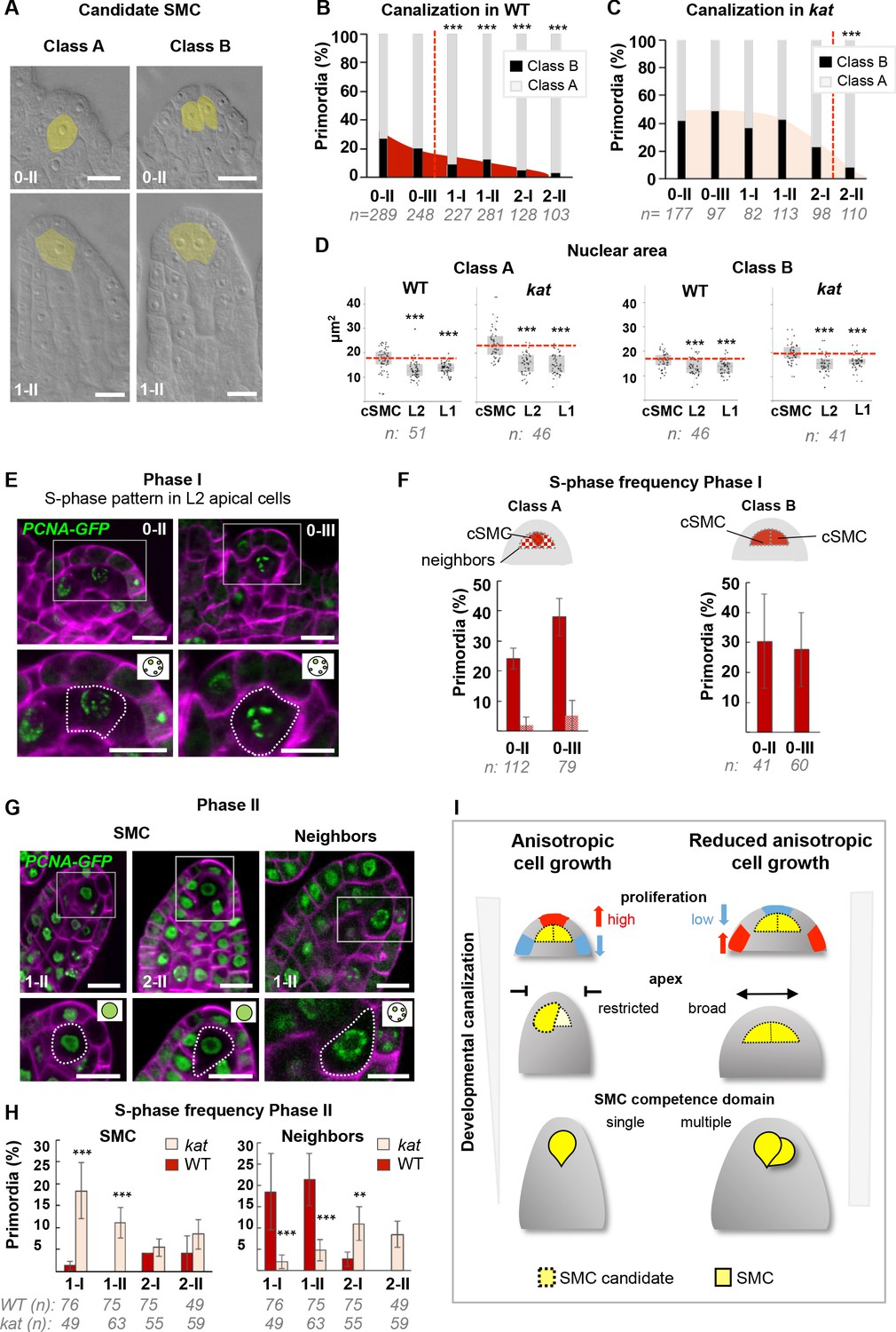
SMC singleness is progressively resolved during primordium growth.
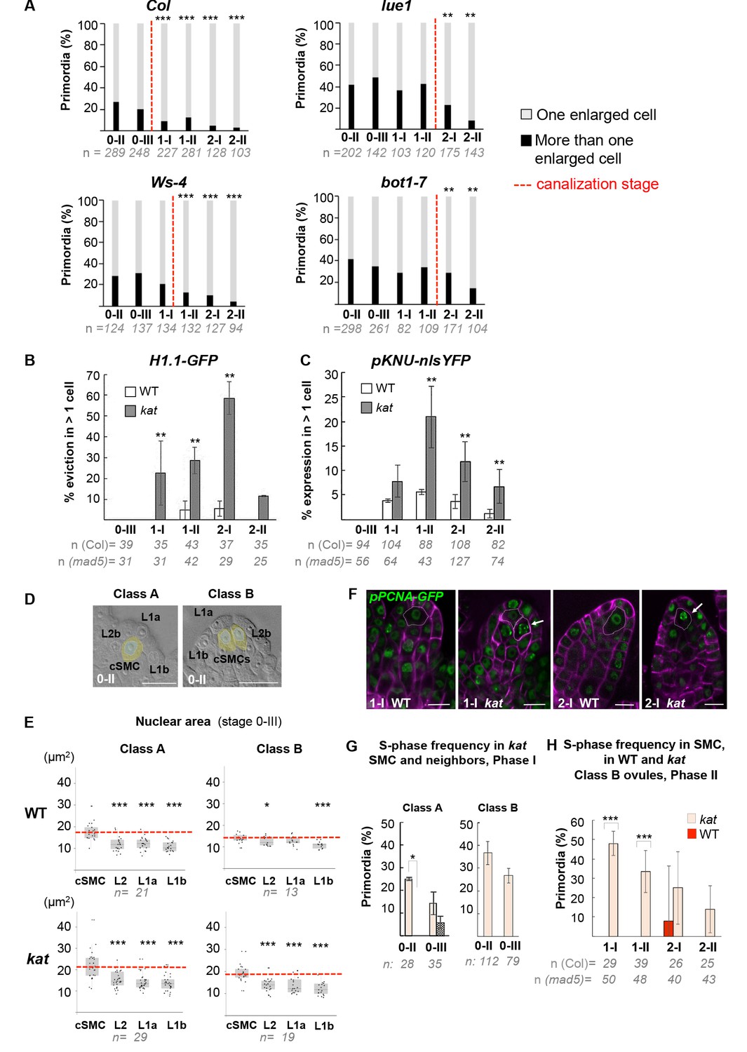
(A–B) In wild-type (WT) plants, ovule primordia harbor one (class A) or occasionally two (class B) SMC candidates with the frequency of class B gradually decreasing during development, reminiscent of developmental canalization. Typical images obtained by tissue clearing with SMC candidates highlighted in yellow (A) and plots showing the percentages of classes A and B (B). The frequency of class B ovules is significantly reduced from stage 1-I, suggesting that canalization (represented by the red dashed line) occurs before that stage. The plot coloration is a visual aid only. (C) Developmental canalization is delayed in kat mutants (mad5 allele). The proportion of class B ovules is significantly reduced from stage 2-II only. Quantifications for two additional kat alleles are presented Figure 6—figure supplement 1A. The plot coloration is a visual aid only. (D) The candidate SMCs initially identified as enlarged cells consistently show an enlarged nucleus in both class A and class B primordia. Nuclear area is compared between the candidate SMCs (cSMC) and surrounding L2 and L1 cells (see Figure 6—figure supplement 1D and Materials and methods for further details). Box plots include jittered data points to visualize data variability. Red lines represent the median of cSMC nuclear area for comparison with other cell types. Equivalent quantifications for stage 0-III are presented in Figure 6—figure supplement 1E. (E–F) During Phase I (stages 0-II, 0-III), S-phase is detected in candidate SMCs at higher frequency than in neighbor cells in Class A ovules, and in both SMC candidates in Class B ovules. Representative images of ovule primordia showing the speckled S-phase pattern of the pPCNA1::PCNA1:sGFP reporter (green) (E). Magenta signal: Renaissance SR2200 cell wall label. Scale bar 10 µm. Quantification of speckled S-phase pattern in the SMC candidate and L2 neighbors (class A ovules) or in both SMC candidates (class B) (F). (G–H) During Phase II (stages 1-I to 2-II), in Class A wild-type ovule primordium, SMC exits S-phase, and neighbor cells undergo S-phase; while kat primordia show the opposite pattern. Representative images of Class A ovule primordia primarily showing the nucleoplasmic pattern of pPCNA1::PCNA1:sGFP in SMCs at stages 1-II (left panel) and 2-II (middle panel); and of the speckled S-phase pattern in neighbor cells (right panel). Quantification of speckled S-phase pattern in SMC candidates and neighbors in Phase II wild-type and kat primordia (I). Representative images and quantifications of Phase I kat primordia and of class B primodia are presented in Figure 6—figure supplement 1F–H. See also Figure 2H. (I) Model for the role of KAT in primordium growth and SMC differentiation (graphical abstract). In WT primordia, SMC differentiation follows a developmental canalization process influenced by cell growth anisotropy that shapes the primordium apex. In kat mutants, reduced anisotropy modifies the cell proliferation pattern, enlarges the apex and the L2,L3 apical domain, leading to multiple SMC candidates (delayed canalization). We propose that ovule primordium shape, controlled by anisotropic cell growth, determines SMC singleness. Images: scale bars: 10 um. Graphs: n = total number of ovules. Error bar: standard error of the mean (F, I). Differences between cell types, domains, or genotypes as indicated in the graphs were assessed using Wilcoxon signed rank test in (D), and a two-tailed Fischer’s exact test in B, C, F, and I. p values: *p≤0.05, **p≤0.01, ***p≤0.001. Quantifications for additional alleles and detailed quantifications are provided in Figure 6—figure supplement 1 and Figure 6—source data 1.
-
Figure 6—source data 1
Raw data for quantitative analysis.
- https://cdn.elifesciences.org/articles/66031/elife-66031-fig6-data1-v2.xlsx
Figure 6—figure supplement 1
SMC singleness is progressively resolved during primordium growth.
(A) Canalization of SMC fate in different katanin (kat) alleles (lue1, bot1-7) and respective wild-type (WT) backgrounds (Col, Ws-4). Percentages of classes A and B primordia based on cleared tissue preparations as shown Figure 6A. The proportion of primordia with several SMC candidates at stage 0-II gradually decreases with developmental progression while the proportion of ovules with a single SMC increases, suggesting canalization. A significant delay in canalization (dashed red line) in kat mutants was confirmed by a two-tailed Fischer’s exact test (see also Figure 2—source data 1). Related to Figure 6B–C. (B–C) Ectopic expression of SMC fate in kat primordia (mad5 allele) compared to WT (Col). Percentage of ovule primordia showing H1.1-GFP eviction (B) and KNU-nlsYFP expression (C) in more than one SMC candidate at all developmental stages. Two-tailed Fischer’s exact test was used to assess differences between genotypes. Related to Figure 6B–C and Figure 6D–E. (D–E) Nuclear area as a marker of SMC candidates. Illustration of the cells selected for nuclear area measurements in representative class A and B ovules (D). Nuclei areas were measured in two L1 cells types (L1a, apical position and L1b, closer to the placenta), in cSMC: candidate SMC; L2b: a neighboring L2 cell. Dashed circles mark the nuclei of these cells used in the measurements. Related to Figure 6D. Quantification of nuclear area as shown in (D) for class A and B in WT (Col) and kat (mad5 allele) ovule primordia at stage 0-III (E). Box plot representations include jittered points to visualize data variability. Red lines represent the median of cSMC nuclear area for comparison with the other cells. Wilcoxon signed rank test was used to assess difference between SMC and the other cell types. Related to Figure 6D. (F–H) Frequency of SMCs showing an S-phase pattern in kat and Class B primordia. (F) Representative images; green, PCNA-GFP, magenta: Renaissance SR2200 cell wall label. Scale bar 10 µm. Related to Figure 6F and H. (G) Quantification of S-phase occurrence in SMCs (salmon bars) and neighbor cells (dashed bars) of class A and class B katanin (mad5) ovule primordia in Phase I (stages 0-II and 0-III). (H) Quantification of S-phase occurrence within the L2 apical domain of class B WT (Col) and kat (mad5 allele) ovule primordia in Phase II (stages 1-I to 2-II). The plotted frequencies refer to the number of primordia showing a speckled PCNA-GFP pattern in SMC candidates. Two-tailed Fischer’s exact test was used to assess differences between genotypes. Related to Figure 6H. All graphs: n = number of ovules scored. Error bar: standard error of the mean. p values: *p≤0.05, **p≤0.01, ***p≤0.001. See also Figure 6—source data 1.
Tables
Table 1
Classification criteria of Arabidopsis ovule primordia.
The table summarizes general characteristics of ovule primordia per stage: cell ‘layers’ above the placenta scored as the number of L1 cells in a cell file drawn from the basis to the top, range thereof, total cell number, ovule shape including height, width, aspect ratio. See also Figure 1—source data 1.
| 0-I | 0-II | 0-III | |||||||
|---|---|---|---|---|---|---|---|---|---|
| Cells above placenta* | 2.5 | (±3.5) | (n = 21) | 3.6 | (±0.5) | (n = 17) | 5.9 | (±1.0) | (n = 11) |
| Range (min-max) | 2 | - | 3 | 3 | - | 4 | 5 | - | 8 |
| Total # cells | 28 | (±5.7) | (n = 21) | 38 | (±8.0) | (n = 17) | 80 | (±8.4) | (n = 11) |
| Width (µm) (W) | 23 | (±3.5) | 26.3 | (±2.4) | 28.0 | (±3.1) | |||
| Height (µm) (H) | 5.3 | (±1.2) | 11.9 | (±2.1) | 22.5 | (±3.6) | |||
| H:W ratio | 0.2 | (±0.04) | (n = 13) | 0.45 | (±0.06) | (n = 14) | 0.8 | (±0.12) | (n = 8) |
| 1-I | 1-II | 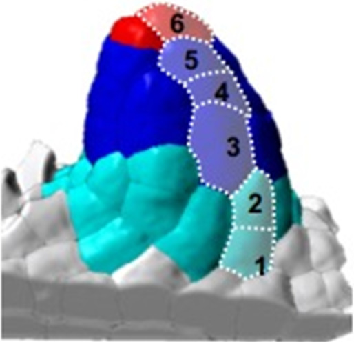 * scoring the length of L1 cell file above placenta | |||||||
| Cells above placenta* | 7.3 | (±1.3) | (n = 15) | 9.7 | (±1.0) | (n = 11) | |||
| Range (min-max) | 6 | - | 10 | 8 | - | 11 | |||
| Total # cells | 105 | (±10.6) | (n = 15) | 128 | (±18.0) | (n = 11) | |||
| Width (µm) (W) | 27 | (±2.0) | 27.8 | (±3.5) | |||||
| Height (µm) (H) | 30 | (±2.8) | 39 | (±5.9) | |||||
| H:W ratio | 1.1 | (±0.10) | (n = 6) | 1.4 | (±0.22) | (n = 8) | |||
| 2-I | 2-II | ||||||||
| Cells above placenta* | 10 | (±1.1) | (n = 10) | 12.6 | (±1.0) | (n = 7) | |||
| Range (min-max) | 9 | - | 12 | 11 | - | 14 | |||
| Total # cells | 151 | (±18.9) | (n = 10) | 165 | (±19.8) | (n = 7) | |||
Table 2
Hypotheses used to generate the mass-spring (MS)- and continuous Finite Element Method (FEM)-based simulations.
Several growth and mechanical hypotheses were listed at start of modeling. To evaluate their effect on primordium growth, each hypothesis was excluded (-) in at least one scenario. The FEM- and MS-based models presented in Figure 3 and Figure 3—figure supplement 1 are numbered according to scenarios 1–8 in the table. Since it is not possible for MS models to simulate material anisotropy, Model 1 was only tested with FEM models. The hypothesis of growth anisotropy is always active for the L1 layer in the models as reported in the table. Empty dots for ‘material anisotropy’ were considered only for the FEM models. See also Figure 3—figure supplement 1 and Appendix 1 for modeling principles, results, and detailed computational methods.
| Modeling hypotheses | Models | ||||||||
|---|---|---|---|---|---|---|---|---|---|
| 1 | 2 | 3 | 4 | 5 | 6 | 7 | 8 | ||
| Growth anisotropy | ● | ● | - | ● | ● | ● | ● | ● | |
| Material anisotropy | ● | - | ○ | ○ | ○ | ○ | ○ | ○ | |
| Strain-based growth | ● | ● | ● | ● | ● | ● | ● | - | |
| Signal-based growth | |||||||||
| Distribution | L1 only | - | - | - | - | - | ● | - | - |
| Inner L2,L3 tissue only (pit-shape) | - | - | - | - | - | - | ● | - | |
| L1 + inner L2,L3 tissue (pit-shape) | ● | ● | ● | - | ● | - | - | ● | |
| L1 + inner L2,L3 tissue (broad distribution) | - | - | - | ● | - | - | - | - | |
| Fixed high concentration | L1 only | - | - | - | - | ● | ● | - | - |
| Inner L2,L3 tissue only | - | - | - | - | - | - | ● | - | |
| L1 + inner L2,L3 tissue | ● | ● | ● | ● | - | - | - | ● | |
Key resources table
| Reagent type (species) or resource | Designation | Source or reference | Identifiers | Additional information |
|---|---|---|---|---|
| Chemical compound, drug | Renaissance SR2200 | Renaissance Chemicals | SCRI Renaissance Stain 2200 | https://www.renchem.co.uk/index.php/specialty-chemicals-division/item/48-selected-fluorescent-dyes-and-brighteners-for-microscopists |
| Chemical compound, drug | PI stain | Sigma- Aldrich | Catalog # P4170 | Propidium Iodide |
| Chemical compound, drug | Na-metabisulphite | Sigma- Aldrich | Catalog # S9000/PubChem: 329824616 | Sodium metabisulphite |
| Chemical compound, drug | Aniline Blue | Sigma- Aldrich | Catalog # 415049 | |
| Other | 3D digital atlas ovule primordium | This paper | https://doi.org/10.5061/dryad.02v6wwq2c | Data resource. 3D segmented images (.ims files) wild-type (Col-0, Ws-4) and katanin (bot1-7) as shown in Figure 1—source data 1 and Figure 4—source data 1 |
| Genetic reagent (Arabidopsis thaliana) | Col-0 | NASC | NASC (RRID:SCR_004576) Stock ID: N22625 | Wild-type ecotype Col-0 |
| Genetic reagent (Arabidopsis thaliana) | Ws-4 | NASC | NASC (RRID:SCR_004576) stock ID: N5390 | Wild-type ecotype Ws-4 |
| Genetic reagent (Arabidopsis thaliana) | bot1-7 | doi:10.1046/j.1365-313x.2001.00946.x | bot1-7 mutant. H.Höfte. | |
| Genetic reagent (Arabidopsis thaliana) | mad5 | doi:10.1126/science.1159151 | mad5 mutant. O.Voinnet. | |
| Genetic reagent (Arabidopsis thaliana) | lue1 | NASC | NASC (RRID:SCR_004576) Stock ID: N57954 | lue1 mutant |
| Genetic reagent (Arabidopsis thaliana) | CYCB1db-GFP | doi:10.1016/j.cub.2009.06.023 | promCYCB1.1::CYCB1.1db-GFP. M.Bennett. | |
| Genetic reagent (Arabidopsis thaliana) | H1.1-GFP | doi:10.1242/dev.095034 | promH1.1::H1.1-GFP. | |
| Genetic reagent (Arabidopsis thaliana) | KNU-nlsYFP | doi:10.1242/dev.075390 | promKNU::nls-YFP. M.Tucker. | |
| Genetic reagent (Arabidopsis thaliana) | DMC1-GUS | doi:10.1046/j.1365-313x.1997.11010001.x | promAtDMC1::GUS. I.Siddiqi. | |
| Genetic reagent (Arabidopsis thaliana) | pWOX2:CENH3-GFP | doi:10.1186/s12870-015-0700-5 | promWOX2::CenH3-GFP. N.DeStorme. | |
| Genetic reagent (Arabidopsis thaliana) | PCNA-GFP | doi:10.1038/srep29657 | promPCNA1::PCNA1-GFP. S. Matsunaga. | |
| Genetic reagent (Arabidopsis thaliana) | pAKV:H2B-GFP | doi:10.1371/journal.pbio.1001155 | promAKV::H2B-GFP. W.C. Yang. | |
| Genetic reagent (Arabidopsis thaliana) | GFP:KTN1 | doi:10.1126/science.1245533 | promKTN1::GFP-KTN1. D.W. Ehrhardt. | |
| Software, algorithm | IMARIS | http://www.bitplane.com/imaris/imaris | RRID:SCR_007370 | 3D image processing software Bitplane AG, Switzerland |
| Software, algorithm | ExportImarisCells, | This paper. | plugin for IMARIS to export segmented cells in meshes for MorphographX. https://github.com/barouxlab/ExportImarisCells (copy archived at swh:1:rev:50badce519f07cf529c3abef765b58972fff70e6); Mosca, 2021a. | |
| Software, algorithm | MorphoGraphX | https://morphographx.org/ | Software to perform 2D/3D segmentation and image analysis | |
| Software, algorithm | MorphoMechanX | https://morphographx.org/morphomechanx/ | Software to perform 2D/3D biomechanical simulations | |
| Software, algorithm | MassSpring Models_ovuleGrowth2D | This paper. | DOI:10.5281/zenodo.4681169 | plugin for MorphoMechanX, 2D MS-models simulation tool. https://github.com/GabriellaMosca/MassSpring_2DovuleGrowthModel (copy archived at swh:1:rev:a66b0496ba51ca7674f0020ace723aa0b850470f); Mosca, 2021b. |
| Software, algorithm | FEM_2DOvule GrowthModel | This paper. | DOI:10.5281/zenodo.4681167 | plugin for MorphoMechanX, 2D FEM-models simulation tool. https://github.com/GabriellaMosca/FEM_2DOvuleGrowthModel (copy archived at swh:1:rev:6b6c09f6039ce3e9d55686d6b6e9dadf28b53e2f); Mosca, 2021c. |
| Software, algorithm | 3DAutoLabeling-ShapeQuant | This paper. | DOI:10.5281/zenodo.4681165 | plugin for MorphoMechanX, automatic labeling of L1, L2, L3 layers and cell shape quantifier. https://github.com/GabriellaMosca/3DAutoLabeling-ShapeQuant (copy archived at swh:1:rev:3138c3fb10891afbc1d48d35395dc00ee58ce199); Mosca, 2021d. |
| Software, algorithm | OvuleViz | This paper. | R-based, shiny interface for interactive plotting of Imaris data. https://github.com/barouxlab/OvuleViz (copy archived at swh:1:rev:fd614aa1e80258928ee036191f26c3dd703d3141); Pires, 2021. | |
| Software, algorithm | R Project for Statistical Computing/RStudio | https://www.r-project.org/ http://www.rstudio.com/ | RRID:SCR_001905 | R Core Team, 2013 |
| Software, algorithm | OMERO | http://www.openmicroscopy.org/site/products/omero | RRID:SCR_002629 | Besson et al., 2019 |
| Software, algorithm | FIJI | http://fiji.sc | RRID:SCR_002285 | Rueden et al., 2017 |
Additional files
Download links
A two-part list of links to download the article, or parts of the article, in various formats.
Downloads (link to download the article as PDF)
Open citations (links to open the citations from this article in various online reference manager services)
Cite this article (links to download the citations from this article in formats compatible with various reference manager tools)
Organ geometry channels reproductive cell fate in the Arabidopsis ovule primordium
eLife 10:e66031.
https://doi.org/10.7554/eLife.66031


