Highly localized intracellular Ca2+ signals promote optimal salivary gland fluid secretion
- Department of Pharmacology and Physiology, University of Rochester, United States
- Department of Veterinary Medicine, College of Bioresource Sciences, Nihon University, Japan
- Department of Mathematics, University of Auckland, New Zealand
Figures
Figure 1
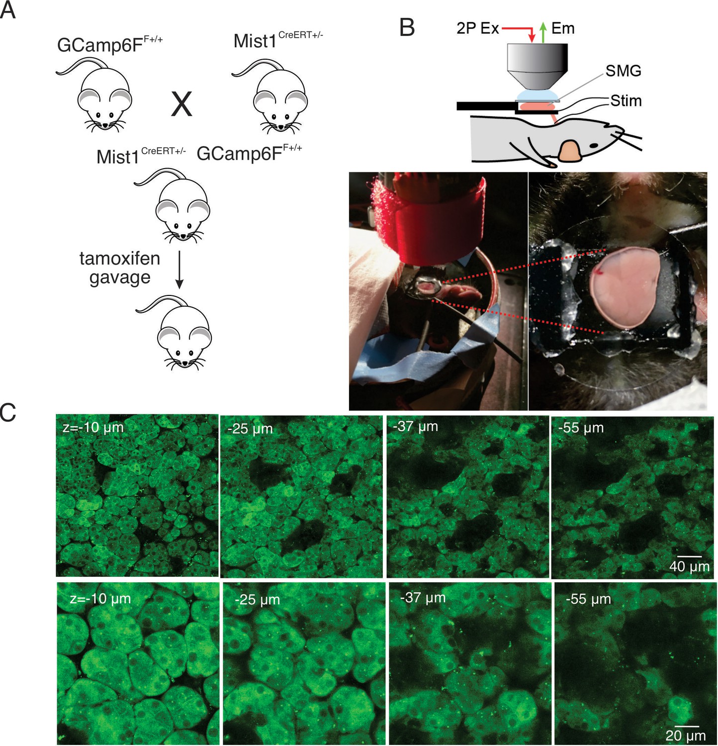
In vivo SMG Ca2+ imaging.
(A) Generation of transgenic mice expressing the GCaMP6f gene driven by Mist1 promotor. GCaMP6f is selectively expressed in acinar cells and appears uniformly through the cytoplasm but is largely excluded from the nucleus. (B) Animal preparation for in vivo imaging. A SMG was lifted and placed on a small platform, then held with a coverslip on top. Stimulation electrodes were inserted to a duct bundle that connect SMG to the body to stimulate nerves that innervate to SMG. (C) A series of z-projection images of SMG with GCaMP (green) expressed in acinar cells.
Figure 2
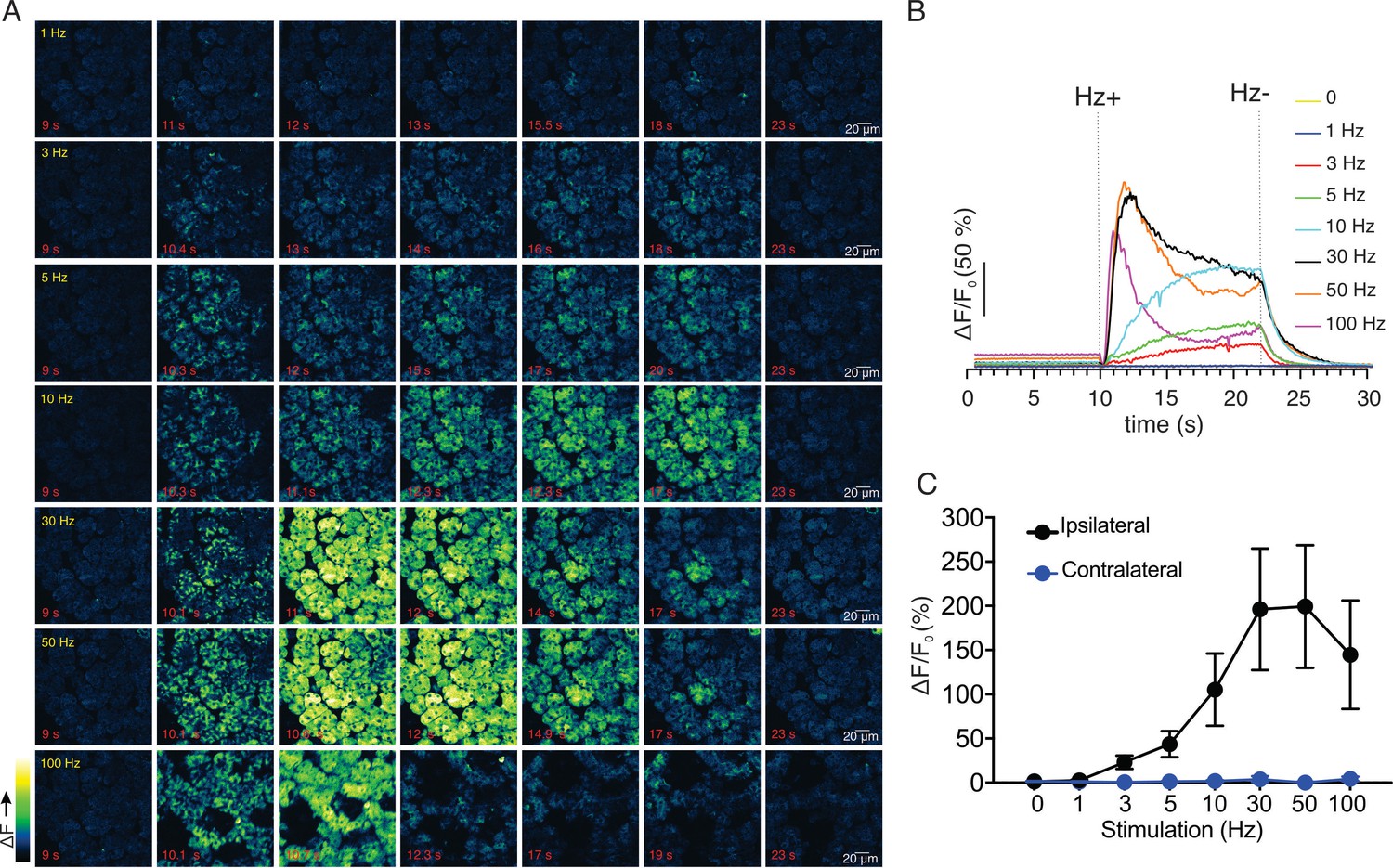
Ca2+ signals evoked in response to nerve stimulation.
(A) Time-course images of Ca2+ (baseline fluorescence was subtracted) in response to 1–100 Hz stimulations. (B) Mean response of the entire field of view to stimulation at the indicated frequency. N = four fields from, four animals. (C) A summary of peak Ca2+ increases during each stimulation. Stimulation was only to the ipsilateral SMG, as the contralateral SMG failed to respond. N = 4 fields from four animals. Mean ± sem. *p <0.05 vs. contralateral gland, t test.
-
Figure 2—source data 1
Source data associated with Figure 2B and C.
- https://cdn.elifesciences.org/articles/66170/elife-66170-fig2-data1-v2.csv
Figure 3
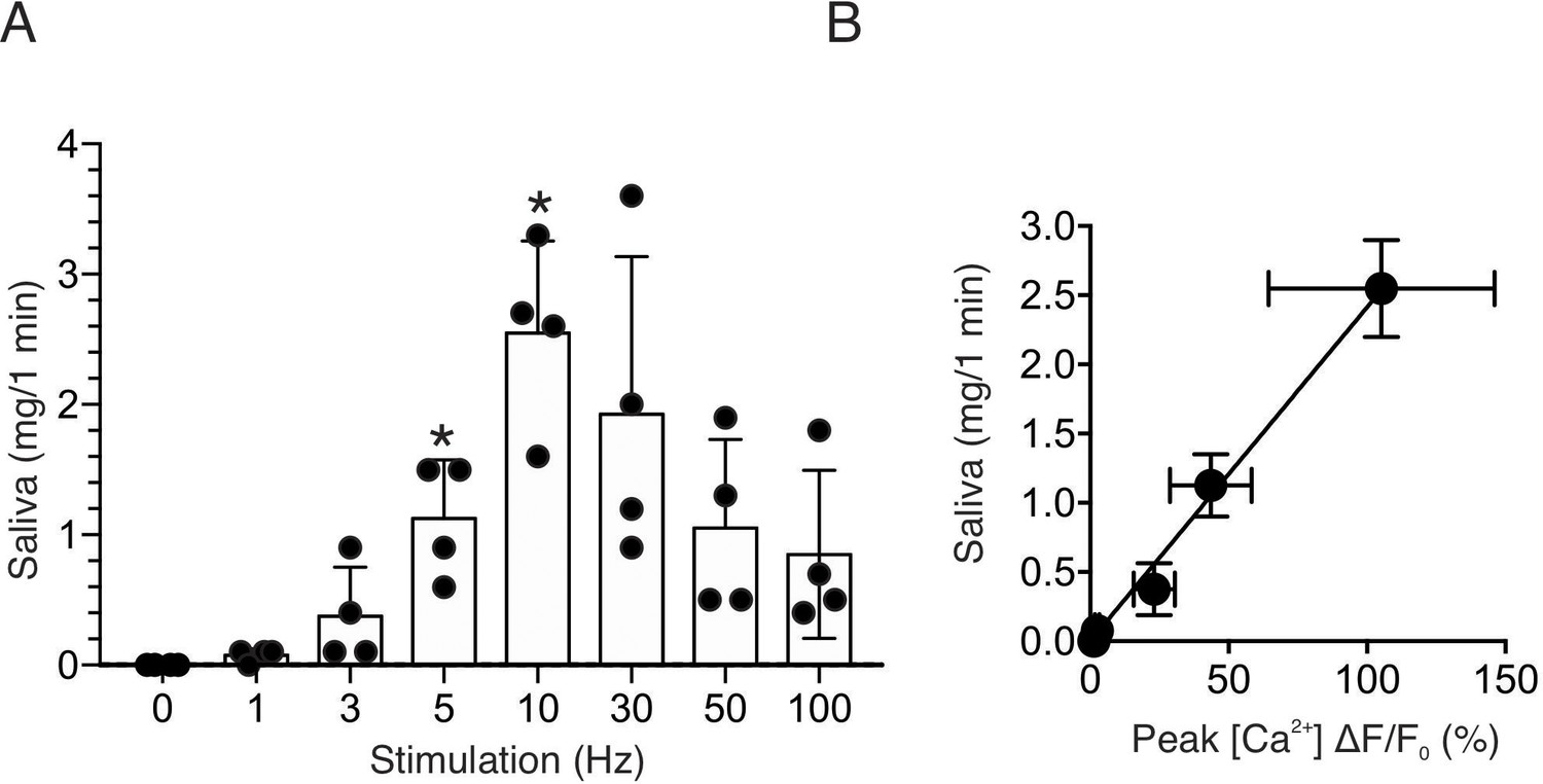
Saliva secretion following nerve stimulation.
(A) A summary histogram of total saliva secretion following 1 min stimulations at the indicated frequency. N = four animals. Mean ± sem. (B) A correlation plot of peak Ca2+ (shown in Figure 2C) vs. saliva secretion, which showed a linear regression of R2 = 0.995 (black line) for stimulation frequency 1–10 Hz. *p <0.05 vs. no stimulation ANOVA with Dunnett test.
-
Figure 3—source data 1
Source data associated with Figure 3A and B.
- https://cdn.elifesciences.org/articles/66170/elife-66170-fig3-data1-v2.csv
Figure 4

Sustained Ca2+ signals are dependent on Ca2+ influx through Orai channels.
(A) Continuous 10 Hz stimulation results in an initial peak followed by a sustained plateau. In animals injected with the Orai channel blocker GSK7975A following the initial stimulation, subsequent stimulation results in a substantial reduction in the sustained phase of the response monitored following 5 min of stimulation. (B/C) shows the pooled data showing the magnitude of [Ca2+] at initial peak (12 s after the initiation of stimulation, left) and sustained phase (5 min after the initiation, right) before and after 20–40 min of vehicle or GSK7975A administration. N = 3–5 from 3 to 5 animals. *p<0.05 paired t test.
Figure 5 with 1 supplement
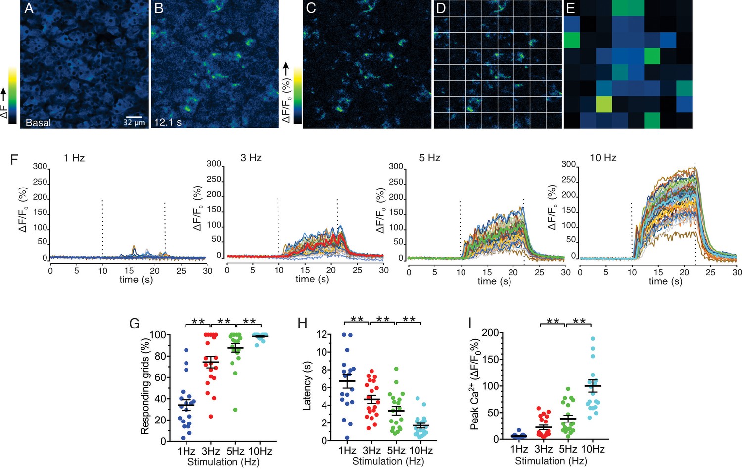
Spatial analysis of Ca2+ responses to various stimulations.
(A–B) An imaging field before (A) and during (B) a stimulation. (C–D) An imaging field was divided to grids of 32 x 32 µm, to yield 64 regions. (E) The average intensity per grid was obtained in each time frame. (F) Representative time-course plots of all 64 grids before, during, and after 1–10 Hz stimulations. Thick colored line represents the mean of the 64 grids for each stimulation. (G) A summary plot of average percent of responding grids in a field by the stimulations. N = 19 fields from eight animals. Mean ± sem. (H) A summary plot of average latencies to initiation of Ca2+ increases in all grids. Non-responding grids were excluded for the data. Mean ± sem. N = 19 from eight animals. (I) A summary plot of average peak Ca2+ increases in all grids. Mean ± sem. N = 19 from eight animals. **p<0.01 ANOVA with Tukey test.
-
Figure 5—source data 1
Source data associated with Figure 5G–I.
- https://cdn.elifesciences.org/articles/66170/elife-66170-fig5-data1-v2.csv
Figure 5—figure supplement 1
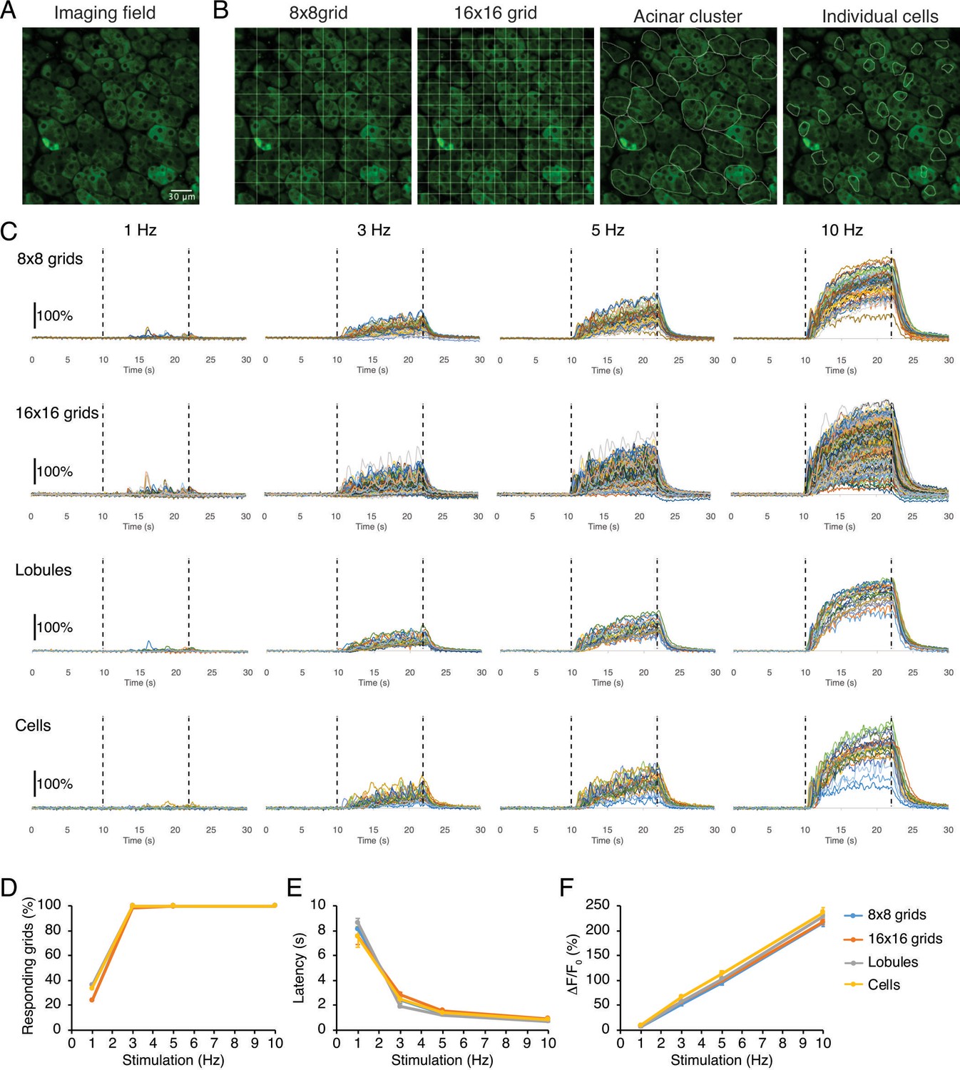
Grid subdivision of imaging field approximates the [Ca2+] behaviors of lobules.
(A) A representative imaging field. (B) 8x8 grids (1012 µm2 per grid) or 16x16 grids (253 µm2 per grid) were applied to the image. In addition, individual lobules (average = 1150 ± 65 µm2) and acinar cells (average 212 ± 12 µm2) were randomly chosen and manually selected as a reference. (C) Time-course traces of [Ca2+] in each grid/lobule before, during, and after 12 s stimulations. (D–F) Analysis showing results obtained from 8x8 grids and 16x16 grids agreed with the results from the lobules/cells.
Figure 6
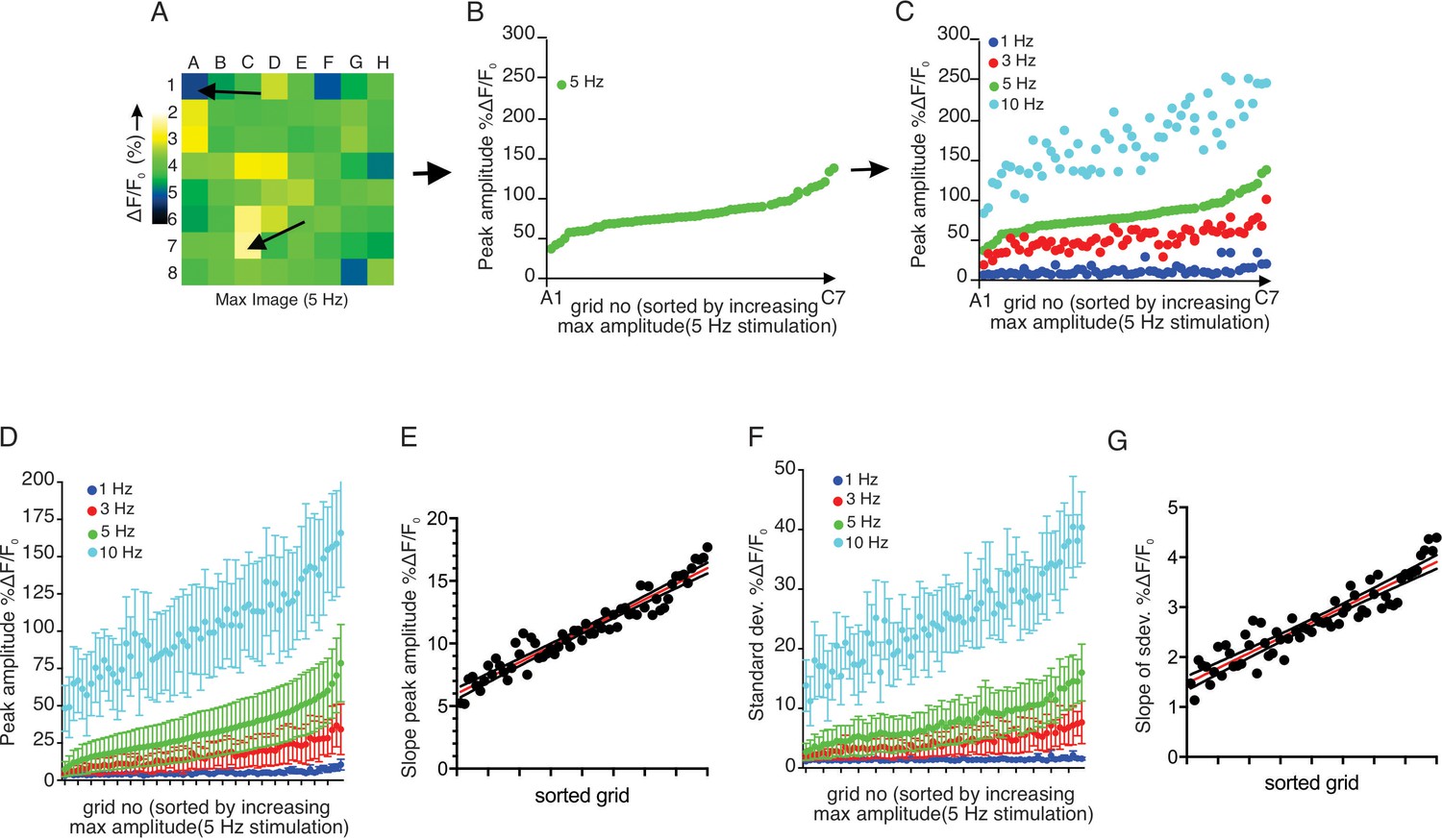
Each sub-divided field possesses unique sensitivity.
(A) An example image of a processed imaging field showing peak intensities during a stimulation in each grid. The grids consist of lowest intensity (arrow, grid A1) to highest (arrow, grid C7). (B) A representative plot of peak Ca2+ increases for each grid in a field to a 5 Hz stimulation. The grids in x axis were reordered from the lowest intensity to the left to the highest on the right. (C) Different stimulation strengths were applied to the same field, and the responses were plotted according to the order indexed by the responses to 5 Hz. (D) A summary plot of peak Ca2+ increases in each grid sorted by responses to 5 Hz. Mean ± sem. n = 5 from four animals. (E) A correlation plot of sorted grid, from low peak Ca2+ to high, vs. degree of Ca2+ increases in response to higher stimulation. Linear regression with R2 = 0.920. N = 5 from four animals. (F) A summary plot of standard deviations of Ca2+ changes during stimulations in each grid sorted by responses to 5 Hz. N = 5 from four animals. Mean ± sem. (G) A correlation plot of sorted grids, from low peak Ca2+ to high, vs. degree of standard deviation of Ca2+ flux in response to higher stimulation. Linear regression with R2 = 0.866. N = 5 from four animals.
-
Figure 6—source data 1
Source data associated with Figure 6D–G.
- https://cdn.elifesciences.org/articles/66170/elife-66170-fig6-data1-v2.csv
Figure 7

Enhancement of Ca2+ responses by cholinesterase inhibition.
(A–D) Representative average traces from 64 grids of changes in Ca2+ responses in a same field before (black) and after (blue) physostigmine. (E) A summary plot of average percent of responding grids in a field by the stimulations in paired fields. N = 5 from four animals. Mean ± sem. (F) A summary plot of average latency to initiation of Ca2+ increases in all grids in paired experiments. Non-responding grids were excluded for the data. N = 5 from four animals. Mean ± sem. (G) A summary plot in paired experiments of average peak Ca2+ rise in all grids. N = 5 from four animals. Mean ± sem. *p<0.05; **p<0.01 Paired t test.
-
Figure 7—source data 1
Source data associated with Figure 7E–G.
- https://cdn.elifesciences.org/articles/66170/elife-66170-fig7-data1-v2.csv
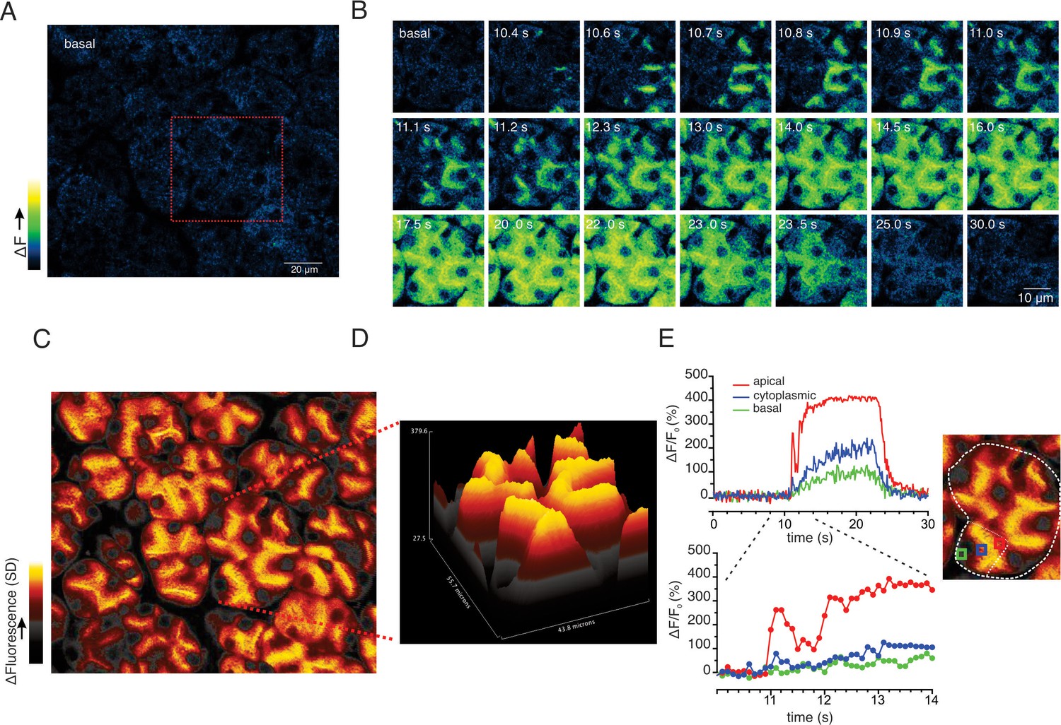
Figure 8 with 1 supplement
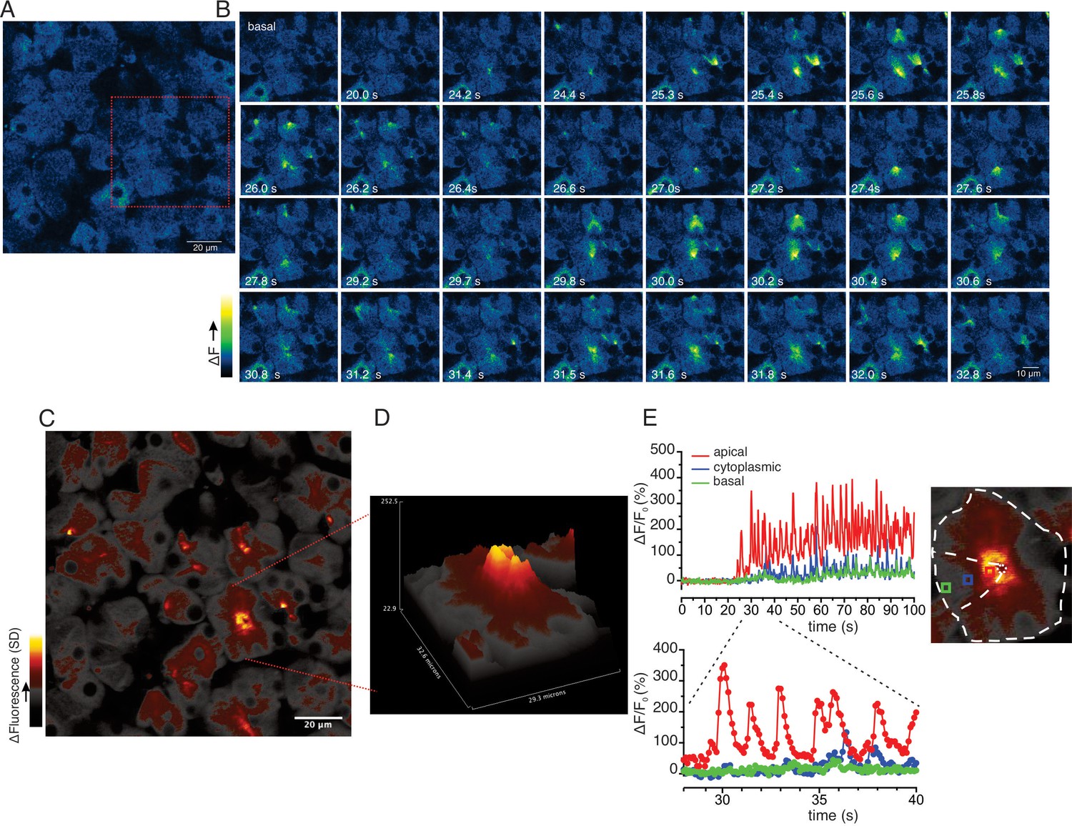
Ca2+ signals are restricted to the apical region during moderate stimulation.
(A) A representative imaging field prior to stimulation. (B) Time-course images of a field containing an acinar cluster (red box in panel A) showing active Ca2+ signaling in the extreme apical portion in the cells. (C) A processed image mapping standard deviation values during stimulation period in the field shown in panel (A). (D) A 3D plot of the SD image of the acinar cluster in B, showing large fluctuations in [Ca2+] only in the apical domain with minimal Ca2+ signal transmission to the basal aspects of the cell. (E) Plot of Ca2+ changes in a single cell from the apical domain (red box in the in the right image), cytoplasmic (blue box in the right image) and basal (green box in right image).
Figure 8—figure supplement 1
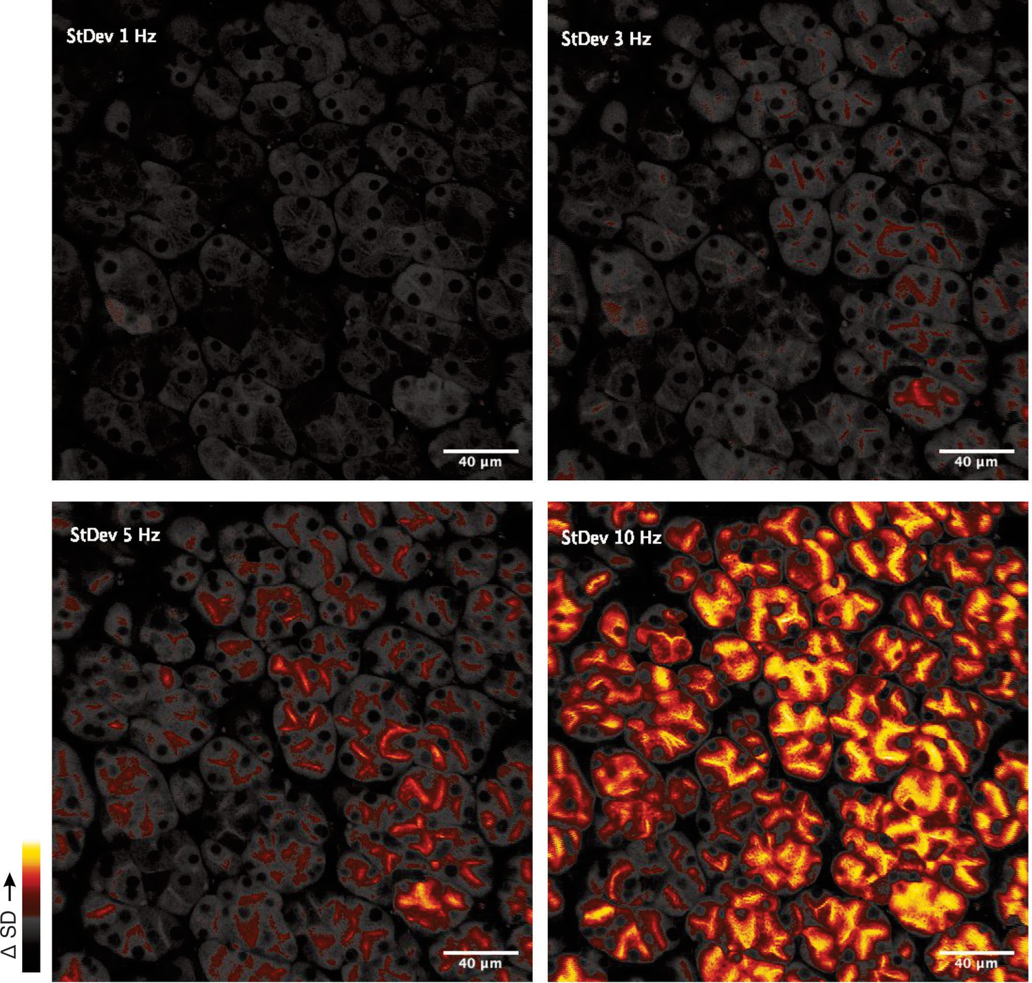
Standard deviation images generated from the image series for the period of stimulation in a single represented imaged field.
At all stimulus intensities, the largest changes in fluorescence are observed in the extreme apical region of the acinar cluster. At lower stimulus intensities, there is no appreciable propagation of the signal to the basal aspects of the cells. At higher intensities (10 Hz) a significant apical-basal gradient is established.
Figure 9
Apical to basal [Ca2+] gradients are established during optimal stimulation.
(A) A representative imaging field prior to stimulation. (B) Time-course images of a field containing an acinar cluster (red box in panel A) depicting predominant Ca2+ changes in the apical portion of cells with smaller changes in the basal regions. (C) A processed image mapping standard deviation values during the stimulation period in the whole field shown in panel (A). (D) A 3D plot of the SD image for the acinar cluster shown in (B). (E) Tracings of Ca2+ changes in the apical domain (red box in the image at right), cytoplasmic (blue box in the image on the right) and basal aspects of a single cell from this cluster (green box in the image at right).
Figure 10

Apical-basal line scans reveal Ca2+ signal spatial homogeneity.
(A) Shows a field of view where the boundaries of an acinus and individual cells have been delimited. The red line indicates the progression of the scan line. (BI, CI and DI) Show consecutive lines stacked in time from left to right for 3, 5 and 10 Hz, respectively. The lower image for each stimulation is an expanded region encompassing the maximum increase in fluorescence for each stimulation. (BII, CII and DII) Show kinetic plots for a 1 pixel 3 μm line placed in the apical, cytoplasmic (prior to the nucleus) and basal (distal to the nucleus) for 3, 5, 10 Hz stimulation, respectively. (BIII, CIII and DIII) Show the profile of the fluorescence along the scan line for the maximum increase in fluorescence for each stimulation frequency expressed as a % of the maximum fluorescence observed at 10 Hz. (E) Shows the pooled data depicting the average increase in apical, cytoplasmic, and basal ROIs at each stimulation frequency. (F) Shows the pooled data for maximal Ca2+ in apical, cytoplasmic, and basal ROIs at each stimulation frequency. White scale bar is 5 μm. ***p<0.001; **p<0.01,* <p< 0.05. Two-way ANOVA with multiple comparisons.
-
Figure 10—source data 1
Source data associated with Figure 10E–F.
- https://cdn.elifesciences.org/articles/66170/elife-66170-fig10-data1-v2.csv
Figure 11
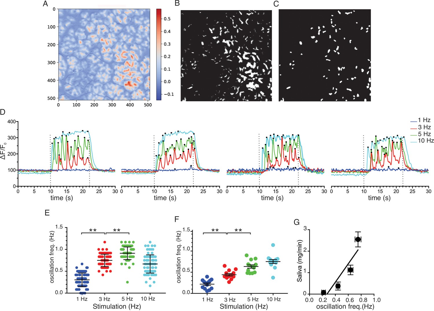
Ca2+ Oscillation frequencies mildly correlates with stimulation strengths.
(A) A representative image generated from averaging signal intensities during a 5 Hz stimulation, which highlights large fluorescence changes in the apical aspects of the cells. (B–C) Mask generated from the image in panel A using Python scripts running in the Jupyter lab environment, as described in Methods. (D) Representative Ca2+ responses from 4 of the ROIs defined in the image in panel C following stimulation at 1–10 Hz. Black dots designate positions of oscillation peaks detected by automated peak detector software written in python. (E) A summary of oscillation frequency of all 79 ROIs from the image in panel A-D. Mean ± sem. (F) A summary plot of oscillation frequencies in response to 1–10 Hz stimulation. N = 13 fields from five animals. Mean ± sem. (G) A correlation plot of oscillation frequency vs. saliva secretion (shown in Figure 3A), which showed a linear regression with R2 = 0.824 (black line). ** p<0.01 ANOVA with Tukey test.
-
Figure 11—source data 1
Source data associated with Figure 11E and F.
- https://cdn.elifesciences.org/articles/66170/elife-66170-fig11-data1-v2.csv
Figure 12 with 1 supplement

Imaging of acutely isolated acinar clusters from GCamp6f expressing SMG at 37°C.
(A) Cells were stimulated with increasing concentrations of CCh. (A) At concentrations greater than 25 nM, repetitive Ca2+ transients were evoked in a minority of cells. (B) Pooled data depicting changes in oscillation frequency with increasing concentrations of carbachol. (C) Pooled data depicting changes in maximum amplitude of CCh- induced Ca2+ signals. (D) Spatial changes in the Ca2+ signal evoked by 25 nM CCh illustrating that the Ca2+ signal is initiated in the extreme apical aspects of the cell and subsequently globalizes to reach the basal domain. (E) Shows a cartoon delimiting the cell shown in D and apical (red box) and basal (black box) ROIs. (F) Shows the kinetic illustrating the apical to basal Ca2+ wave. * p<0.05; **p<0.001 One-way ANOVA.
Figure 12—figure supplement 1
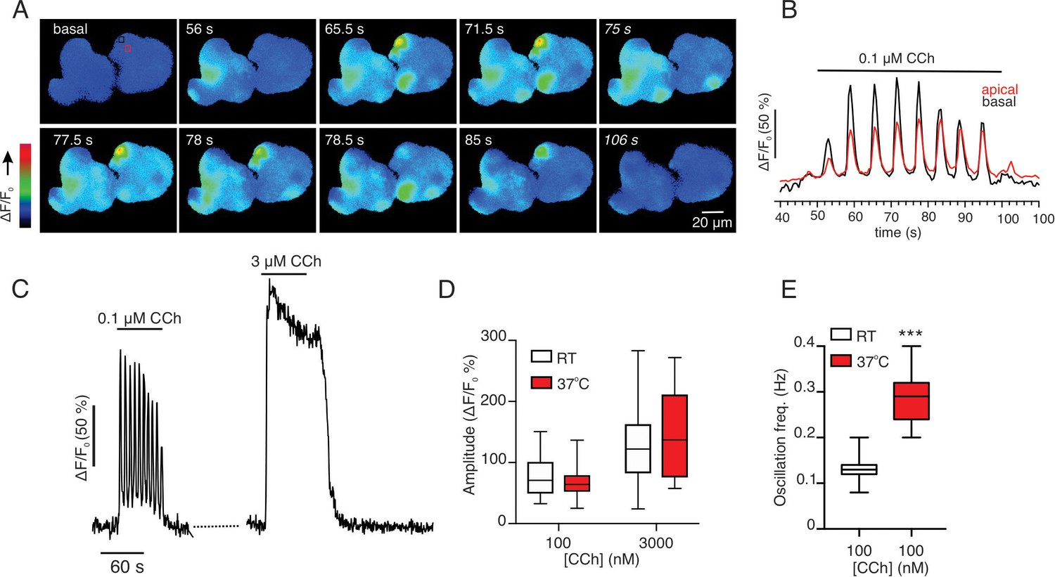
In vitro imaging of acutely isolated acinar clusters isolated from GCamp6F expressing cells at room temperature.
(A) Images taken at the indicated times following stimulation with 100 nM CCh showing that Ca2+ signals are invariably global. (B) Shows the kinetic from an apical (red box) and a basal (black box) following stimulation with 100 nM CCh. (C) Kinetic of response of a single cell to 100 nM and 3 μM CCh. (D) Comparison of maximum amplitude evoked by 100 nM and 3 μM CCh at room temperature and 37°C. (E) Comparison of oscillation frequency evoked by 100 nM at room temperature and 37°C. Pooled data. *** p< 0.001. Welch’s t test.
Figure 13
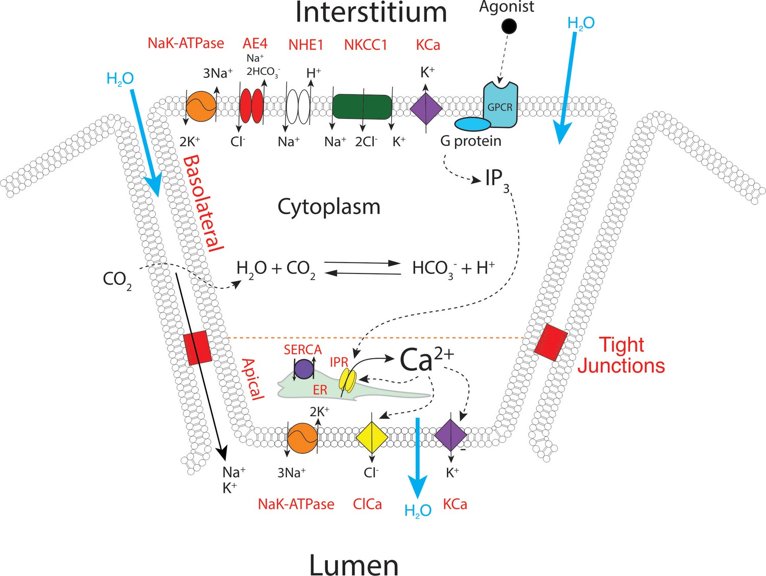
A proposed updated model for salivary secretion.
The mathematical model is based on the fluxes and processes shown here. In contrast to previous models, the apical region now contains all the machinery needed for saliva secretion, included KCa channels and Na/K ATPases. Ca2+ is released predominantly in the apical region, from IP3R that are situated in close proximity to TMEM16a, and there is no requirement for a propagated wave of increased [Ca2+] across the cell.
Figure 14 with 1 supplement
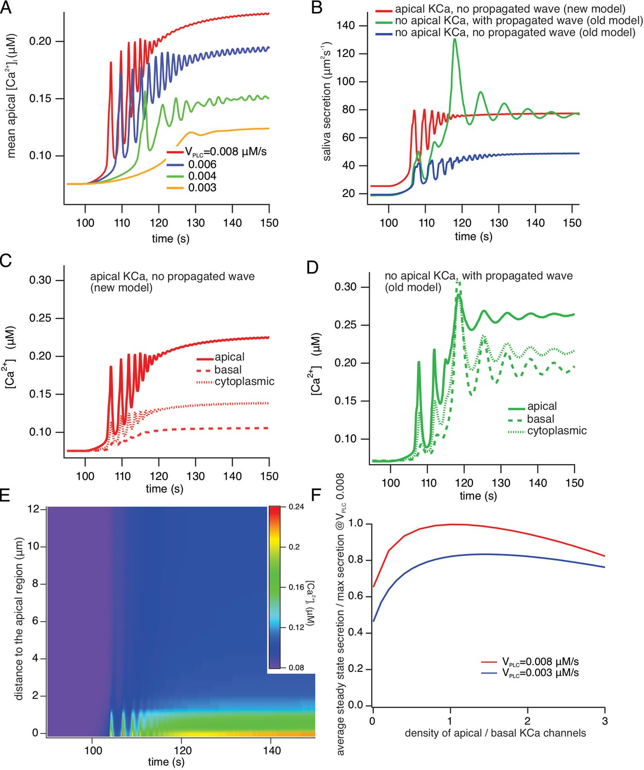
A comparison of model simulations incorporating new data.
(A) Average apical [Ca2+] in the new model for four different values of VPLC (which is a proxy for stimulation frequency). The stimulus was applied at t=100 s. As the stimulus increases the model oscillations increase in frequency, and are superimposed on an increasing baseline, as seen experimentally. (B) Fluid secretion in the new model compared to two versions of the old model of Vera-Sigüenza et al., 2019. When the propagating intracellular Ca2+ wave is removed from the old model (which has no apical KCa channels), secretion decreases significantly. (C and D) [Ca2+] traces averaged from three different regions of the cell in the new model and the old model of Vera-Sigüenza et al., 2019. (E) Line scan constructed from model simulations of the new model with VPLC = 0.008 μM/s. The stimulus was applied at t = 100 s. A line was drawn through the cell from the average of all the apical points to the average of all the basal points, and all grid points within 0.2 μm of this line were selected. The Ca2+ traces from each of these grid points was then plotted as a color density plot, and laid side by side in order of distance from the apical region. The limited spatial resolution is a result of the limited spatial resolution of the grid, as only 36 grid points were close enough to the apical/basal line to be included in the line scan plot. The Ca2+ responses are mostly confined to the apical region, although diffusion does cause a smaller basal response, as seen also in panel (F) Steady-state saliva secretion in the new model as a function of the relative density of apical KCa channels (relative to the density of basal KCa channels) at various vPLC. For all simulations the total number of KCa channels was the same. When there are no apical KCa channels (i.e. when the relative density is zero), fluid flow is decreased by approximately 35%. However, too many apical KCa channels also decreases secretion. Maximal secretion is attained approximately when the KCa channels have the same density in the apical and basal membranes. Note that, if the intracellular propagating Ca2+ wave is removed from the old model it has a similar structure to the new model with no apical KCa channels. However, because of the presence of RyR in the old model, and because of the Ca2+ dependence of PLC in the old model, there remain significant quantitative discrepancies between the old and new models even when they have a superficially similar structure.
Figure 14—figure supplement 1
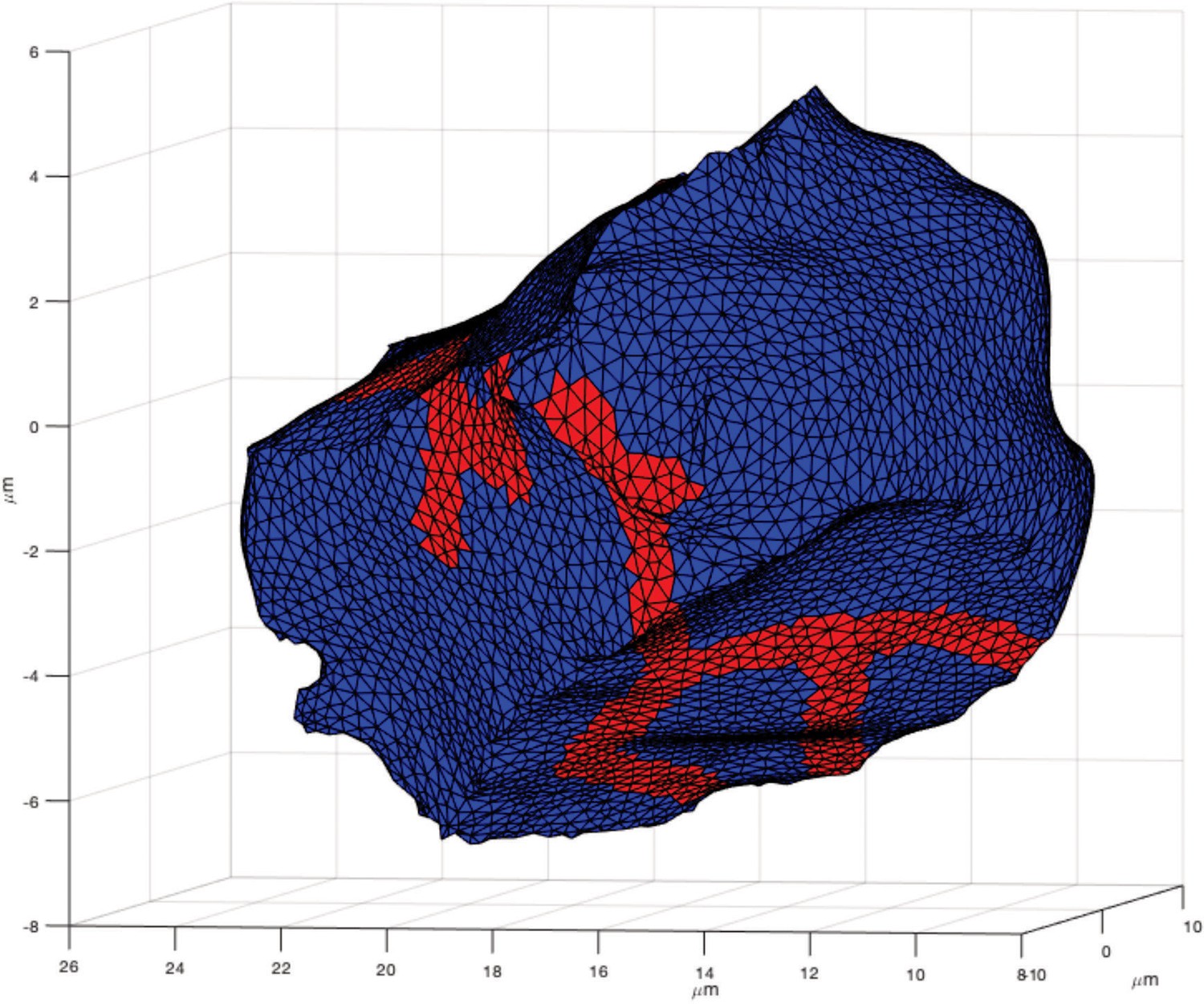
The three-dimensional model cell upon which all the computations in this paper were performed.
The surface of the cell is divided into two regions, one corresponding to the apical membrane (red) and the remainder corresponding to the basolateral membrane (blue). For all the computations here, the model makes no distinction between the basal and lateral membranes. This cell corresponds to cell 4 of Vera-Sigüenza et al., 2019. TMEM Cl- channels are present only on the apical membrane (at a constant density), while KCa channels are distributed on both the apical and basolateral membranes (at varying relative densities, as shown in Figure 14F). All other ion transporters and channels are distributed uniformly on the cell surface, although their spatial distribution is unimportant, as all ions except Ca2+ are assumed to be spatially uniform.
Videos
Video 1
Movie generated by Python scripts running in the Jupyter lab environment following stimulation at 1 Hz.
Left panel shows ΔF/F0 image series. Bottom right panel depicts the change in F/F0 for the apical ROIs automatically generated by the software described in Figure 11.
Video 2
Movie generated by Python scripts running in the Jupyter lab environment following stimulation at 3 Hz.
Left panel shows ΔF/F0 image series. Bottom right panel depicts the change in F/F0 for the apical ROIs automatically generated by the software described in Figure 11.
Video 3
Movie generated by Python scripts running in the Jupyter lab environment following stimulation at 5 Hz.
Left panel shows ΔF/F0 image series. Bottom right panel depicts the change in F/F0 for the apical ROIs automatically generated by the software described in Figure 11.
Video 4
Movie generated by Python scripts running in the Jupyter lab environment following stimulation at 10 Hz.
Left panel shows ΔF/F0 image series. Bottom right panel depicts the change in F/F0 for the apical ROIs automatically generated by the software described in Figure 11.
Video 5
Movie showing ΔF/F0 images from acutely isolated acinar clusters from GCamp6f expressing cells exposed to 25 nM (25–100 s), 50 nM (150–225 s), and 100 nM CCh (275–350 s).
Tables
Key resources table
| Reagent type (species) or resource | Designation | Source or reference | Identifiers | Additional information |
|---|---|---|---|---|
| Strain, strain background (mouse) | B6J.Cg-Gt(ROSA)26Sortm95.1(CAG-GCaMP6f)Hze/MwarJ | Jackson Laboratory | RRID:IMSR_JAX:028865 | |
| Strain, strain background (mouse) | B6.129-Bhlha15tm3(cre/ERT2)Skz/J | Jackson Laboratory | RRID:IMSR_JAX:029228 | |
| Chemical compound, drug | Physostigmine | Tocris Bioscience | 0622 | |
| Chemical compound, drug | GSK7975A | Sigma-Aldrich | 5.34351 | |
| Chemical compound, drug | Carbachol | Sigma-Aldrich | 1092009 | |
| Software, algorithm | FIJI/ImageJ | https://imagej.net/software/fiji/ | ||
| Software, algorithm | Prism | GraphPad | ||
| Software, algorithm | Jupyter Notebook | Jupyter labhttps://jupyter.org/ | ||
| Software, algorithm | SciPy | https://www.scipy.org/ | ||
| Software, algorithm | scikit-image | scikit-image https://scikit-image.org | ||
| Other | Tamoxifen | Sigma-Aldrich | T5648 | |
| Other | Collagenase Type II | Worthington Biochemical | LS004204 |
Additional files
Download links
A two-part list of links to download the article, or parts of the article, in various formats.
Downloads (link to download the article as PDF)
Open citations (links to open the citations from this article in various online reference manager services)
Cite this article (links to download the citations from this article in formats compatible with various reference manager tools)
Highly localized intracellular Ca2+ signals promote optimal salivary gland fluid secretion
eLife 10:e66170.
https://doi.org/10.7554/eLife.66170


