How human runners regulate footsteps on uneven terrain
- Department of Mechanical Engineering and Materials Science, Yale University, United States
- National Centre for Biological Sciences, Tata Institute of Fundamental Research, India
Figures
Figure 1
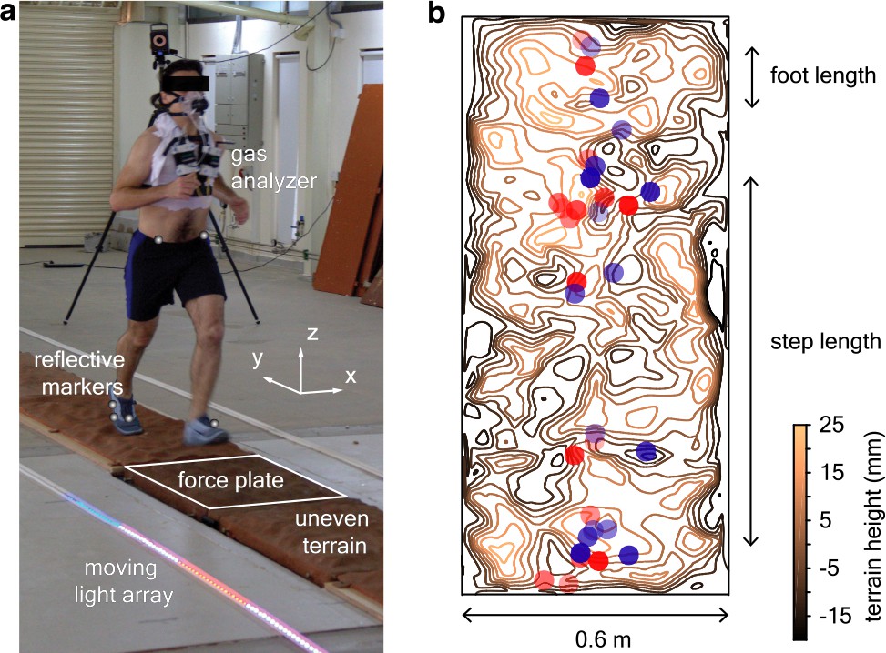
Uneven terrain experiments.
(a) We conducted human-subject experiments on flat and uneven terrain while recording biomechanical and metabolic data. The reflective markers and the outline of the force plate are digitally exaggerated for clarity. (b) Footsteps were recorded to determine whether terrain geometry influences stepping location, illustrated here by a mean-subtracted contour plot of terrain height for an approximately 6 foot segment of uneven II overlaid with footsteps (location of the heel marker). Blue and red circles represent opposite directions of travel and transparency level differentiates trials.
-
Figure 1—source data 1
Dimensional mass and leg length of every subject.
- https://cdn.elifesciences.org/articles/67177/elife-67177-fig1-data1-v2.csv
Figure 2

Details of the experiment design.
(a) Schematic of the running track, camera placement, force plate positions and the LED strip with a 3 m illuminated section. (b) The terrain was designed so that the range of its height distribution was comparable to ankle height and peak-to-peak distances (along the length of the track) were comparable to foot length . (c) Histograms of the mean subtracted heights of the uneven terrain. (d) Histograms of the peak-to-peak separation of the uneven terrain.
Figure 3 with 1 supplement

Foot placement analysis.
(a) Red circles denote footstep locations (392 footsteps) in the ‘’ plane for a representative trial on uneven II. The grid spacing is 190 mm along the length of the track and 95 mm along its width. Step length s0 is shown for reference. is the length of the capture volume and is the width of the track. Note that the and axes of this figure are not to the same scale. (b) The probability of landing on a foot-sized region of the track is quantified by the foot placement index Equation 5 shown as a heatmap with the color bar at the top left.
-
Figure 3—source data 1
Footstep counts for each subject on all terrain.
- https://cdn.elifesciences.org/articles/67177/elife-67177-fig3-data1-v2.pdf
Figure 3—figure supplement 1
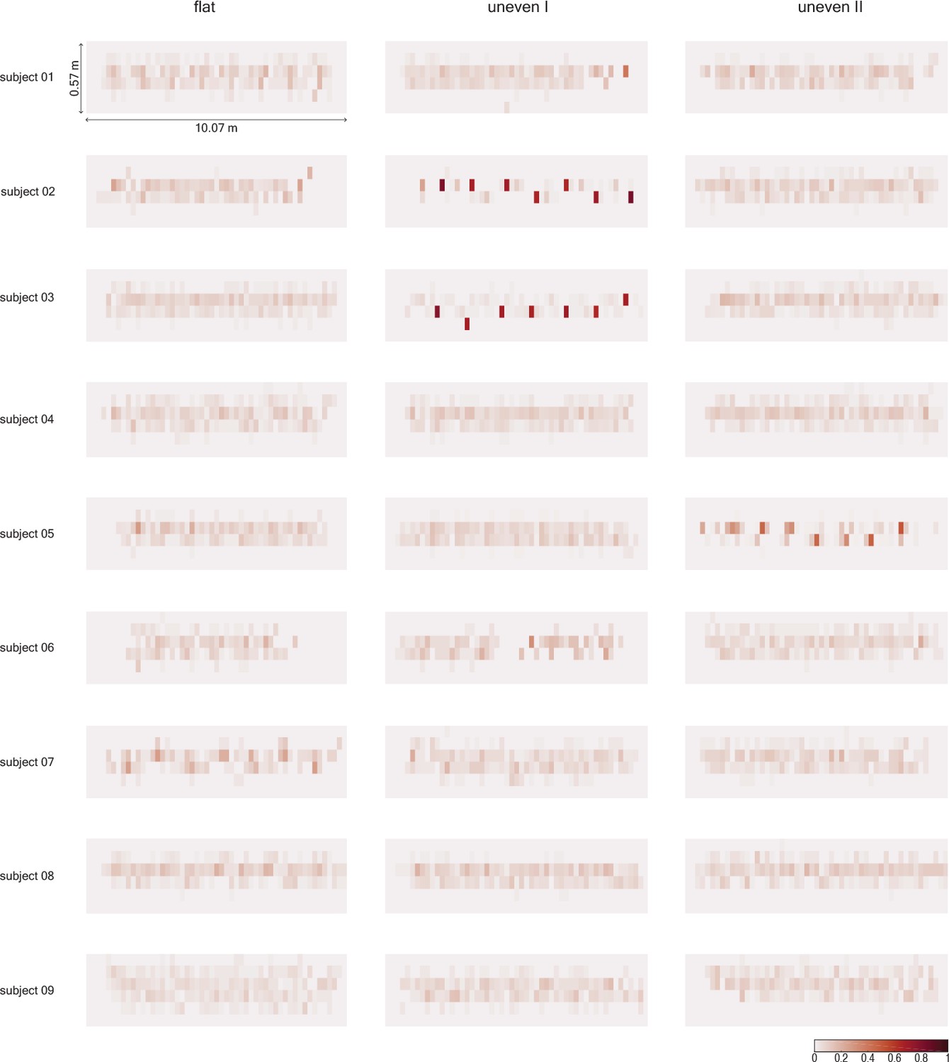
Subject-wise foot placement patterns.
Heatmaps of the foot placement index for all subjects on each terrain. Each cell has an area of 190 mm × 95 mm, with the longer side along the length of the track. Color bar at the bottom right of the figure shows the value of .
Figure 4
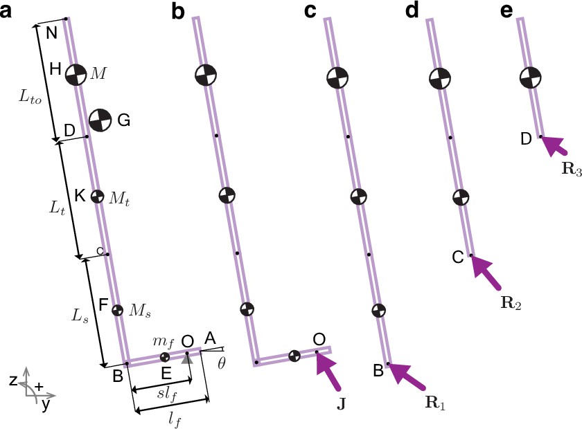
Model for estimating fore-aft collision impulses from kinematic data.
(a) A four-link model of the foot (A–B), shank (B–C), thigh (C–D), and torso (D–N) moving with center of mass velocity and angular velocity collides with the ground at angle . (G) represents the center of mass. Leg length and body mass are obtained from data and scaled according to Dempster, 1955, to obtain segment lengths and masses. Free-body diagrams show all non-zero external impulses: (b) collisional impulse acting at O, and panels (c, d, e) show reaction impulses , , and acting at B, C, and D, respectively.
Figure 5 with 3 supplements
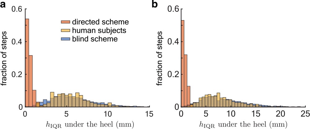
Foot placement on uneven terrain.
Histogram of the interquartile range of heights () at footstep locations for the directed sampling scheme (red), experiments (yellow), and the blind sampling scheme (blue) on (a) uneven I (2526 footsteps) and (b) uneven II (2736 footsteps). Note that varies over a greater range on uneven II.
-
Figure 5—source data 1
Output of the Markov chain sampling (directed scheme) of the Uneven I terrain.
- https://cdn.elifesciences.org/articles/67177/elife-67177-fig5-data1-v2.csv
-
Figure 5—source data 2
Output of the Markov chain sampling (directed scheme) of the Uneven II terrain.
- https://cdn.elifesciences.org/articles/67177/elife-67177-fig5-data2-v2.csv
-
Figure 5—source data 3
Output of the uniform random sampling (blind scheme) of the Uneven I terrain.
- https://cdn.elifesciences.org/articles/67177/elife-67177-fig5-data3-v2.csv
-
Figure 5—source data 4
Output of the uniform random sampling (blind scheme) of the Uneven II terrain.
- https://cdn.elifesciences.org/articles/67177/elife-67177-fig5-data4-v2.csv
-
Figure 5—source data 5
Subject-wise, per-step data of the terrain height at foot landing locations on the Uneven I terrain.
- https://cdn.elifesciences.org/articles/67177/elife-67177-fig5-data5-v2.csv
-
Figure 5—source data 6
Subject-wise, per-step data of the terrain height at foot landing locations on the Uneven II terrain.
- https://cdn.elifesciences.org/articles/67177/elife-67177-fig5-data6-v2.csv
Figure 5—figure supplement 1
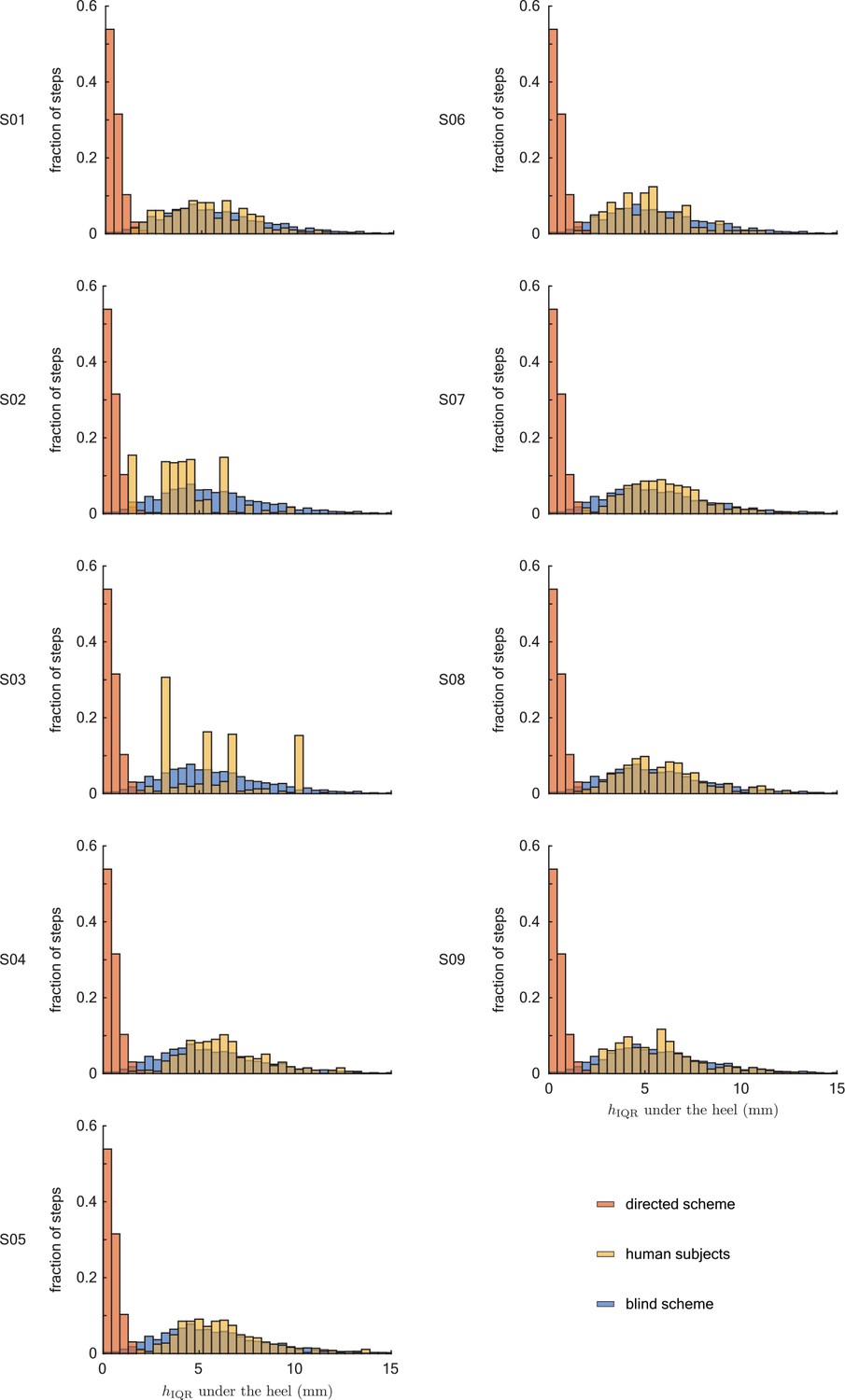
Subject-wise foot placement analysis on uneven I.
Histograms of the interquartile range of heights at the footstep locations for the directed sampling scheme (red), each subject from the experiments (yellow), and the blind sampling scheme (blue).
Figure 5—figure supplement 2
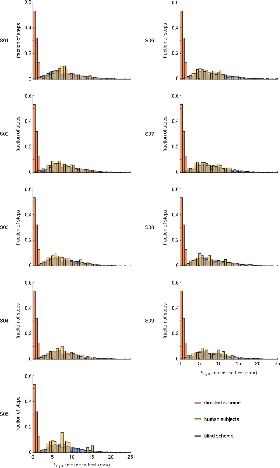
Subject-wise foot placement analysis on uneven II.
Histograms of the interquartile range of heights at the footstep locations for the directed sampling scheme (red), each subject from the experiments (yellow), and the blind sampling scheme (blue).
Figure 5—figure supplement 3
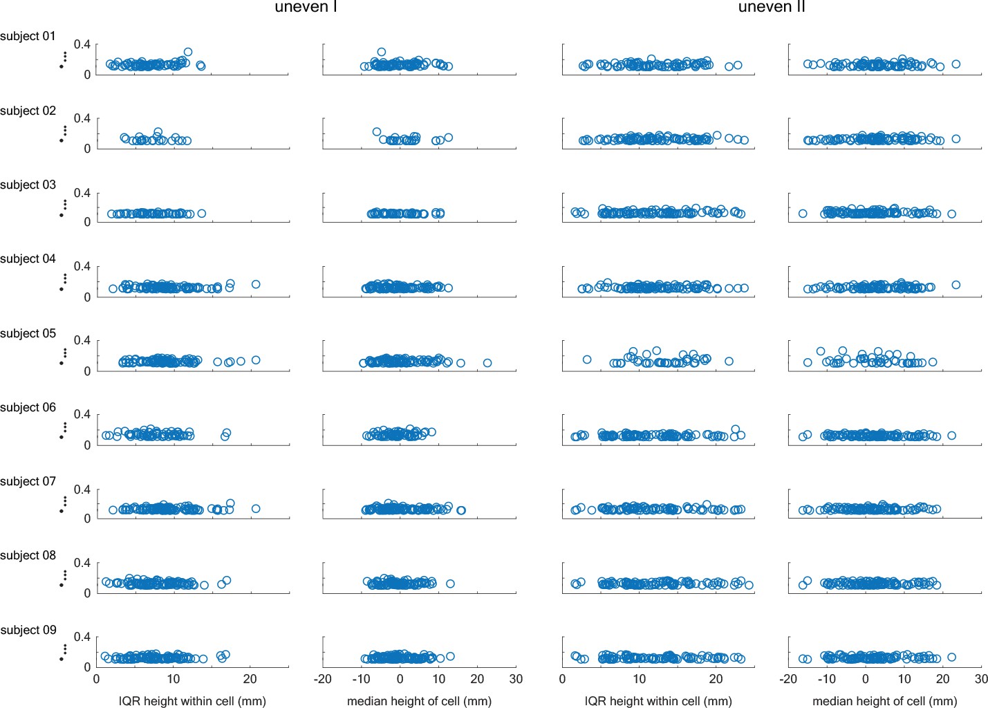
Subject-wise foot placement analysis.
Foot placement index plotted against the median height of the terrain cell and the interquartile range of heights within the terrain cell at landing for all recorded steps on uneven I and uneven II.
Figure 6 with 1 supplement
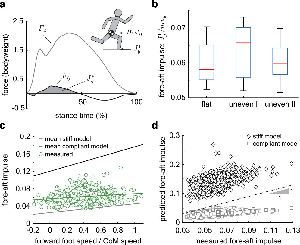
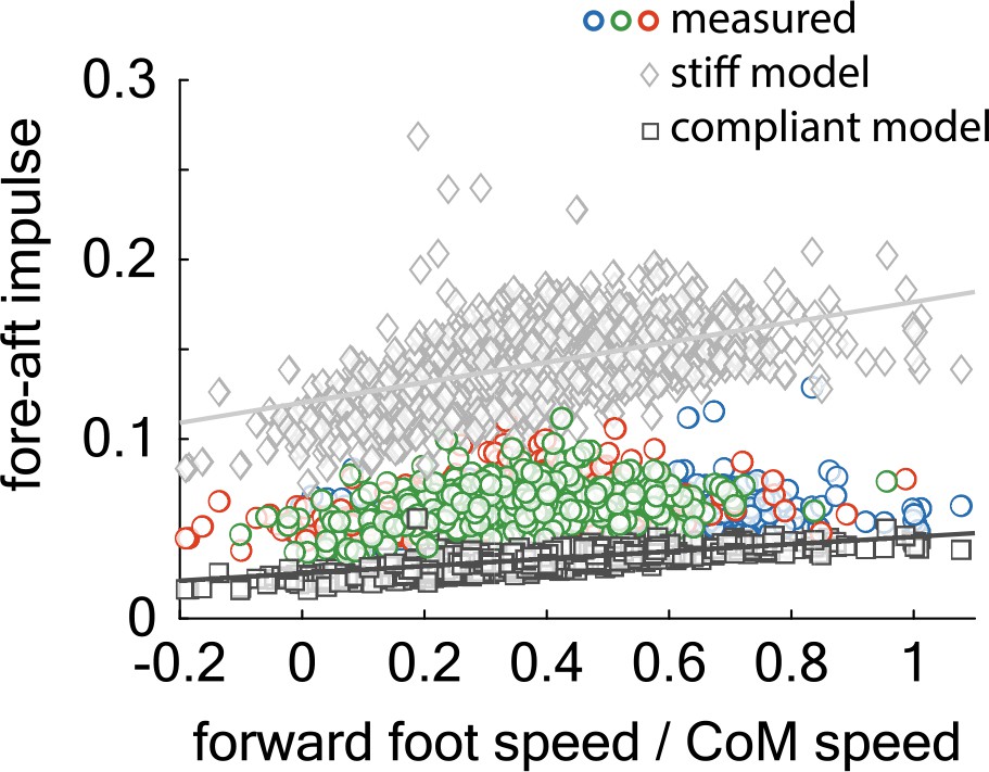
Regulation of fore-aft impulses.
(a) The fore-aft impulse (gray shaded area) is found by integrating the measured fore-aft ground reaction force (black curve) during the deceleration phase. (b) Mean for 9 subjects on 3 terrain types. Central red lines denote the median, boxes represent the interquartile range, whiskers extend to 1.5 times the quartile range, and open circles denote outliers. (c) Measured (green circles) versus relative forward foot speed at landing (forward foot speed/center of mass speed) for each step recorded on all terrain types (total 1081 steps). The green line is the regression fit for the data. The dark and light gray lines are the predicted fore-aft impulse for the mean stiff and compliant jointed models, respectively. Per step model predictions in Figure 6—figure supplement 1. (d) Measured versus predicted fore-aft impulses for every step. The dotted line represents perfect prediction.
-
Figure 6—source data 1
Subject-wise, per-step data of fore-aft impulse, foot speed, and touchdown angle.
- https://cdn.elifesciences.org/articles/67177/elife-67177-fig6-data1-v2.csv
-
Figure 6—source data 2
Per-step data of the measured and predicted fore-aft impulse for the compliant and stiff-leg collision models.
- https://cdn.elifesciences.org/articles/67177/elife-67177-fig6-data2-v2.csv
Figure 6—figure supplement 1
Detailed results of the collision analysis.
Measured (blue circles: flat, red circles: uneven I, green circles: uneven II) and calculated values for the collision model with a compliant leg (dark gray squares) and rigid leg (light gray diamonds) versus relative forward foot speed at landing (forward foot speed/center of mass speed) for each step recorded on all terrain types (total 1081 steps). Solid lines are regression fits to the model. The intercept and slope of the fitted line for the compliant jointed model are 0.0252 ± 0.004 and 0.0203 ± 0.010, respectively (R2 = 0.57, p < 0.0001), and the intercept and slope of the fitted line for the stiff jointed model are 0.120 ± 0.002 and 0.056 ± 0.005, respectively (R2 = 0.29, p < 0.0001).
Figure 7 with 2 supplements
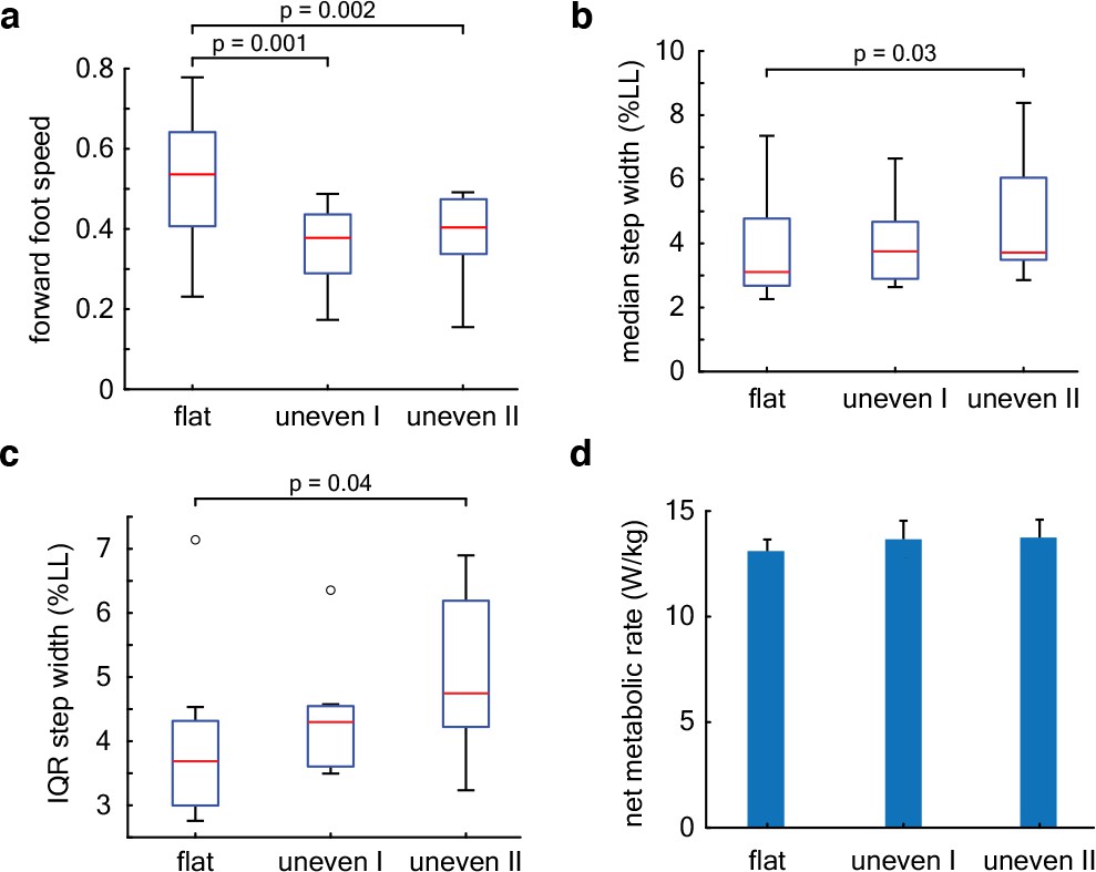
Energetics and stepping kinematics.
(a) Box plot of the mean forward foot speed at landing (units of froude number). (b) Box plot of the median step width (normalized to leg length). (c) Box plot of the step width variability. Central red lines denote the median, boxes represent the interquartile range, whiskers extend to 1.5 times the quartile range, and open circles denote outliers. The distribution of step widths within a trial deviated from normality and hence we report the median and the interquartile range of the distribution for each trial (Figure 7—figure supplement 1), instead of the mean and standard deviation as is reported for all other variables. (d) Net metabolic rate normalized to subject mass. Whiskers represent standard deviation across the nine subjects. An ANOVA on the linear mixed model described in Equation 10 was used to determine whether gait measures described above differed between terrain conditions with a significance threshold of 0.05.
-
Figure 7—source data 1
Subject-wise, per-step data on step width.
- https://cdn.elifesciences.org/articles/67177/elife-67177-fig7-data1-v2.csv
Figure 7—figure supplement 1
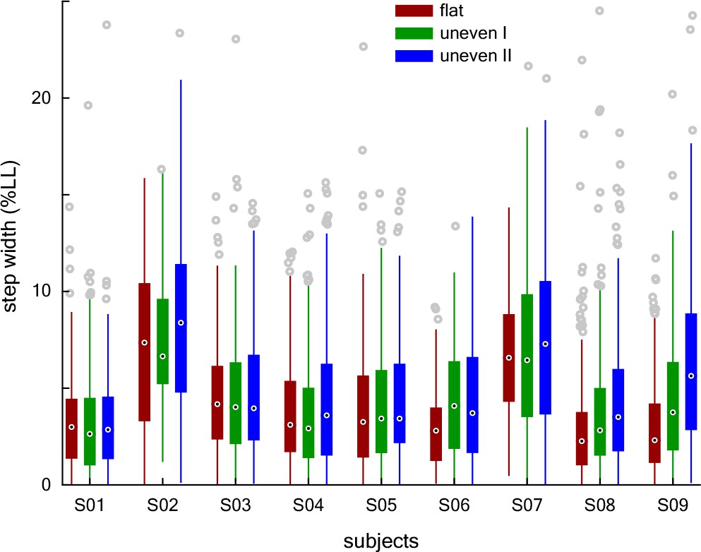
Subject-wise step width statistics.
Step width is expressed as percent leg length (LL). Because the data are skewed with long tails away from zero, we report the median and interquartile range as measures of the central tendency and variability, respectively. Black dots represent medians, boxes show the interquartile range, lines extend to 1.5 times the quartile range, and gray circles represent outliers.
Figure 7—figure supplement 2
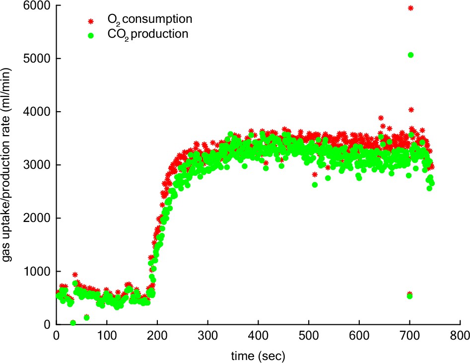
Representative respirometry data.
Breath-by-breath respirometry data for a representative subject running on uneven II. Red stars represent O2 consumption rate and green octagons represent CO2 production rate.
Tables
Table 1
Correlation between landing probability and terrain unevenness.
| Independent variable | DenDF | F-value | p-Value |
|---|---|---|---|
| IQR terrain height | 20.6 | 3.03 | 0.10 |
-
Table 1—source data 1
Subject-wise statistics of the terrain’s height in heel-sized patches and the probability of stepping in that patch.
- https://cdn.elifesciences.org/articles/67177/elife-67177-table1-data1-v2.csv
Table 2
Kinematic variables on different terrain types reported as mean ± SD, except for meander values which are reported as median ± interquartile range.
| Variable | Flat | Uneven I | Uneven II | F-value | p-Value |
|---|---|---|---|---|---|
| Net metabolic rate (W/kg) | 2.97 | 0.08 | |||
| Median step width (%LL) | 4.53 | 0.03 | |||
| IQR step width (% LL) | 3.65 | 0.05 | |||
| Mean step width (%LL) | 8.69 | 0.003 | |||
| SD step width (% LL) | 5.54 | 0.01 | |||
| Mean step length (%LL) | 1.07 | 0.37 | |||
| SD step length (%LL) | 0.64 | 0.54 | |||
| Mean meander () | 1.48 | 0.25 | |||
| SD meander () | 1.58 | 0.23 | |||
| Mean fwd. foot speed (froude num.) | 13.08 | 0.0004 | |||
| SD fwd. foot speed (froude num.) | 1.48 | 0.26 | |||
| Mean CoM speed (m/s) | 2.32 | 0.13 | |||
| SD CoM speed (m/s) | 2.00 | 0.17 | |||
| Mean touchdown leg length (%LL) | 4.28 | 0.03 | |||
| SD touchdown leg length (%LL) | 1.32 | 0.29 | |||
| Mean touchdown leg angle (rad) | 3.90 | 0.04 | |||
| SD touchdown leg angle (rad) | 2.10 | 0.15 |
-
Table 2—source data 1
Subject-wise, per-step data on foot and leg kinetics and kinematics.
- https://cdn.elifesciences.org/articles/67177/elife-67177-table2-data1-v2.csv
Table 3
Details of the ANCOVAs performed on the linear model described in Equation 11 showing the denominator degrees of freedom, F-value and p-value for the fixed terrain factor, and the estimated slopes for the fixed forward foot speed effect.
| Dependent variable | Factor | DenDF | F-value | p-Value | |
|---|---|---|---|---|---|
| Touchdown leg angle | Terrain | 193 | 1.48 | 0.23 | - |
| Fwd. foot speed | 38 | 115.83 | <0.0001 | 0.07±0.01 rad | |
| Fore-aft impulse | Terrain | 79 | 1.45 | 0.24 | - |
| Fwd. foot speed | 78 | 12.83 | 0.001 | 0.01±0.003 |
Additional files
Download links
A two-part list of links to download the article, or parts of the article, in various formats.
Downloads (link to download the article as PDF)
Open citations (links to open the citations from this article in various online reference manager services)
Cite this article (links to download the citations from this article in formats compatible with various reference manager tools)
How human runners regulate footsteps on uneven terrain
eLife 12:e67177.
https://doi.org/10.7554/eLife.67177


