Structural heterogeneity of cellular K5/K14 filaments as revealed by cryo-electron microscopy
- Department of Biochemistry, University of Zurich, Switzerland
- Department of Cell and Developmental Biology, Northwestern University Feinberg School of Medicine, United States
- Institute of Biology, University of Leipzig, Germany
Figures
Figure 1 with 2 supplements
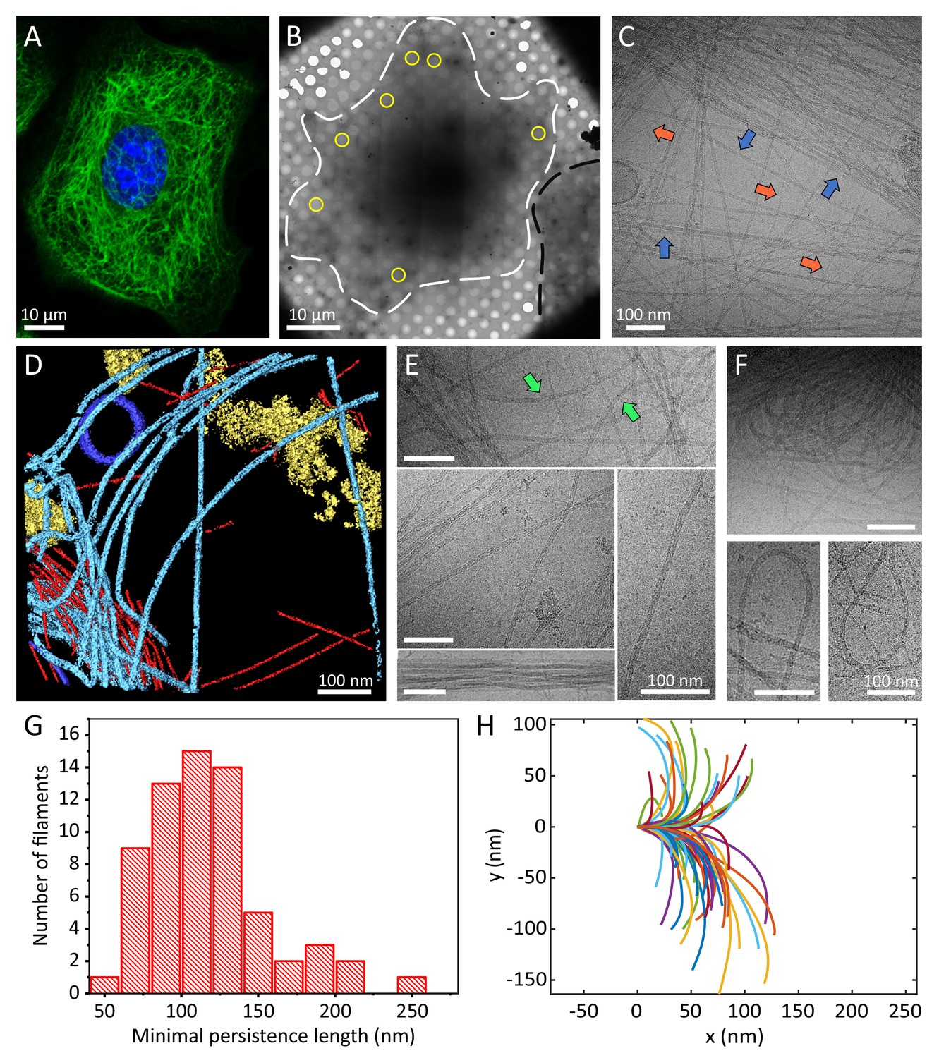
Cellular K5/K14 filaments as revealed by light and cryo-electron microscopy.
(A) The murine keratinocyte cell line K5/K14_1 expressing only K5 and K14 filaments forms a complex KIF meshwork, as revealed by confocal immunofluorescence. Cells were stained for K14 (green) and chromatin (blue). (B) Ghost cells were analyzed by cryo-EM and cryo-ET. Low-magnification image of a cell grown on an EM-grid and treated with detergent prior to vitrification. Cell boundaries (dashed white line) are detected as well as a neighboring cell (dashed black line). Typical regions that were analyzed by cryo-EM are marked (yellow circles). (C) A typical cryo-EM micrograph of a ghost cell imaged at a higher magnification allows the detection of keratin filaments and other cytoskeletal elements (n=1860). Keratin filaments (blue arrows) and actin filaments (orange arrows) are distinguished by their characteristic diameter. A large keratin bundle is visible in the top right corner. (D) Surface rendering view of a cryo-tomogram of a ghost cell (n=44). Keratin filaments (light blue), actin filaments (red), vesicles (dark blue), and cellular debris (yellow) were manually segmented. (E) Different organizations of keratin filaments observed in the cryo-EM micrographs (n=1860), including straight filaments (middle), curved (top, green arrows) and bundled filaments (bottom left). Scale bars: 100 nm. (F) Highly bent keratin filaments are found within cryo-EM micrographs of ghost cells. Scale bars: 100 nm. (G) Quantification of the minimal apparent persistence length measurements performed on (n=65) highly bent keratin filaments extracted from cryo-EM micrographs. (H) A plot combining 65 contours of filaments that were used for the minimal apparent persistence length measurements in (G). Individual filaments, shown in different colors, are aligned at their origins for visualization purposes.
Figure 1—figure supplement 1
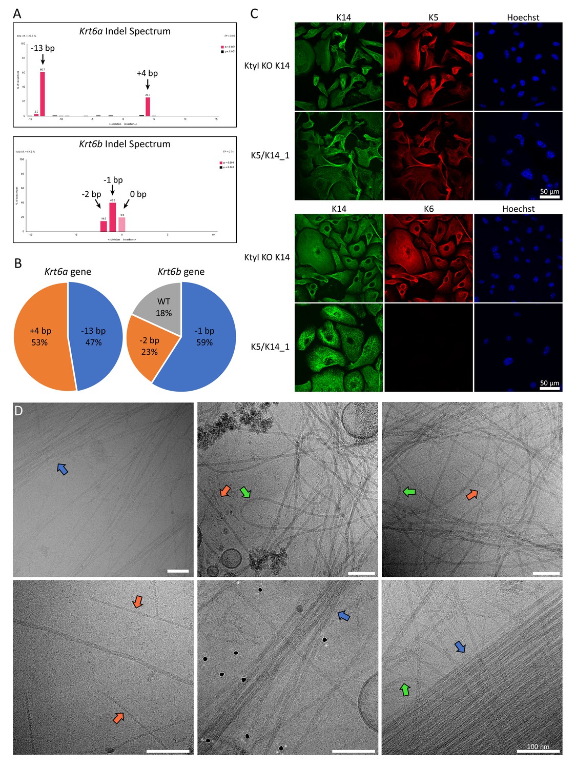
Knockout of K6 isoforms by CRISPR/Cas9.
(A) TIDE analysis of the Krt6a and Krt6b gene sequences of the K5/K14_1 cell line carrying the mutations induced by non-homologous end joining. Genomic DNA fragments of the Krt6a and Krt6b gene were amplified by PCR and sequenced. Peaks in the Indel spectrum confirm mis-sense insertion or deletion mutations in each gene. For Krt6a, a deletion of 13 base pairs (bp) and an insertion of 4 bp were detected, while for the Krt6b gene a deletion of 2 bp and 1 bp were detected, as well as the wild-type sequence. (B) Pie chart plot of the frequency of mutations that were detected in the Krt6a and Krt6b gene of the K5/K14_1 cell line. For this analysis, PCR amplified fragments of genomic Krt6a and Krt6b DNA were ligated into the pGEM T-Easy vector and transformed into bacteria. Bacterial clones which took up individual plasmids carrying a specific mutation were cultivated and the plasmids were extracted individually and analyzed. For the Krt6a gene, 19 bacterial clones were analyzed, for the Krt6b gene, 22 bacterial clones were analyzed. (C) Immunofluorescence analysis of KtyI KO K14 cells and K5/K14_1 cells co-stained for K5 (red) and K14 (green) or K6 (red) and K14 (green). DNA was labeled with Hoechst 33342 (blue). No filamentous K6 network could be detected in the K5/K14_1 cells. Scale bars: 50 µm. (D) Representative cryo-EM micrographs of the K5/K14 network in K5/K14_1 ghost cells. Keratin filaments can be clearly distinguished from actin filaments (orange arrows). Keratin bundles (blue arrows) and very wavy filaments (green arrows) are highlighted. Scale bars: 100 nm.
Figure 1—figure supplement 2
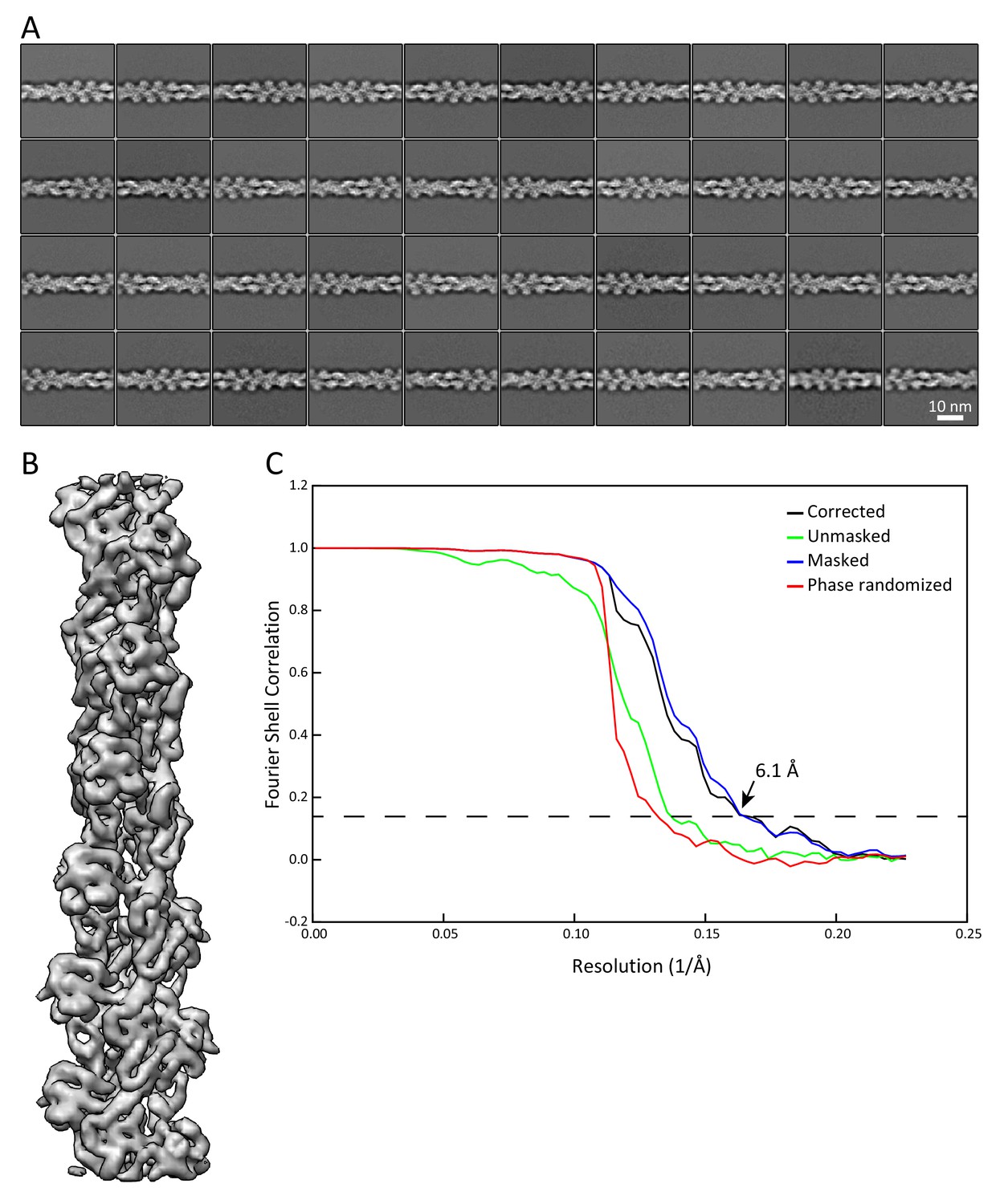
Validation that the sample preparation allows us to retrieve data at sub-nanometer resolution.
Analysis of actin filaments detected in the K5/K14_1 ghost cells served as internal quality control for the sample preparation and the acquired cryo-EM data. Actin filaments were detected around keratins and analyzed independently. (A) Representative 2D classes of F-actin segments of 36 nm length. (B) 3D refined structure of an in vivo assembled actin filament with a resolution of 6.1 Å. Individual α-helices can be recognized. (C) Fourier shell correlation (FSC) plot of the structure shown in (B). The plot shows the unmasked (green), masked (blue), phase randomized (red), and masking-effect corrected (black) FSC curves. The resolution at which the gold-standard FSC curve drops below the 0.143 threshold is indicated.
Figure 2 with 1 supplement

The architecture and heterogeneity of keratin filaments.
(A) Ten of the most populated 2D class averages of keratin segments. High electron density is shown in white. Arrows indicate transition regions between helical and straight-line patterns. In total, 50 classes containing keratin segments (n=305,495) were collected (Figure 2—figure supplement 1A). (B) Distribution of filament diameters as measured in 50 2D class averages (Figure 2—figure supplement 1A). On the y-axis, the number of individual particles that constituted the 2D classes is plotted. (C) Mean intensity line-profile through all classes used in (B). The mean filament diameter (10.1 nm) is indicated and was measured between the zero-crossings of the curve. (D) Subset of keratin class averages showing larger filament diameters. Two individual filamentous densities are often detected within a filament (yellow arrowheads). Additionally, transition regions between thinner and thicker filament regions are detected (white arrows). (E) Intensity line-profiles through a narrow and a wide class indicated by blue and black asterisk (in (A) and (D)), respectively. Diameters of 10.1 nm and 13.2 nm (arrow) were detected. (F) Autocorrelation spectra of the displayed keratin classes (insets). Peaks of the autocorrelation function corresponding to the distance between repetitive elements along the filament (pitch) are indicated (arrows). (G) To show that out-of-plane tilting of KIFs can shift the autocorrelation peaks, Class 24 was tilted in silico by 34°, while Class 10 is untilted. The apparent pitch of both classes is indicated. (H) Autocorrelation spectra of the classes shown in (G). After tilting of Class 24 by 34°, both classes show an autocorrelation peak at the same marked position, an indicator that filament tilting might be the reason for the different pitches observed in the 2D classes. Green and black dots indicate which curve belongs to which class in (G). (I) Dependence of the apparent pitch length (autocorrelation peaks) on the filament tilt angle, measured by tilting Class 24 from 0° to 50° and calculating corresponding autocorrelation spectra. The gray area indicates the range of pitches found in keratin 2D classes.
Figure 2—figure supplement 1
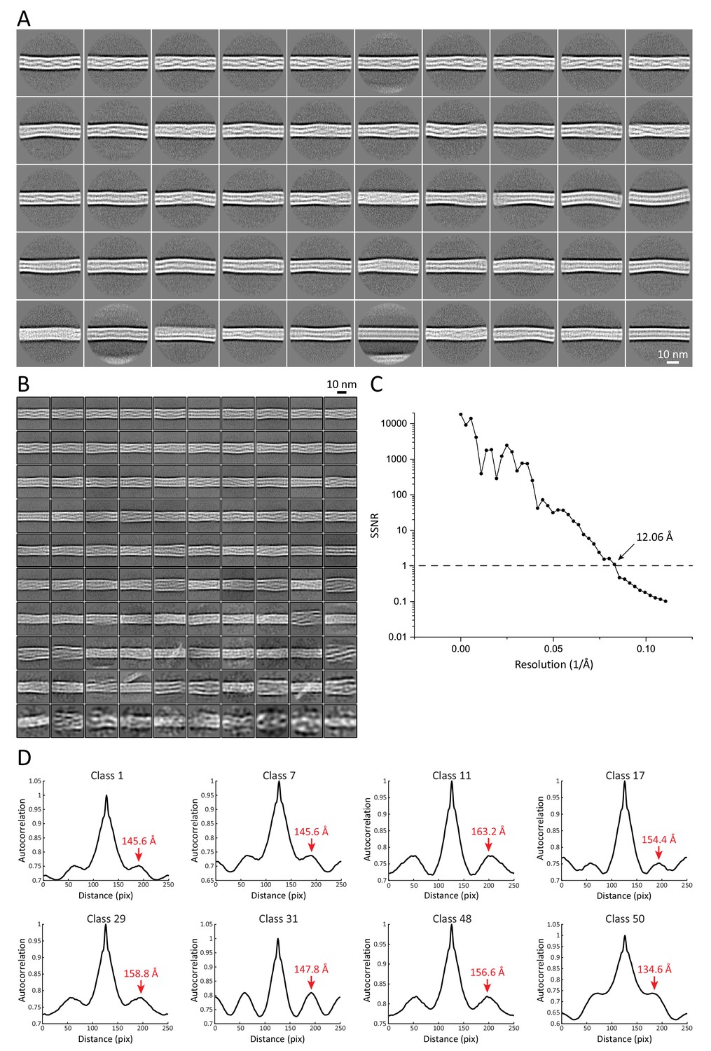
2D structural analysis of keratin segments.
(A) Representative 2D class averages of 55 nm long keratin segments. These classes were used for measurements of filament diameter, mean intensity-line profiles and autocorrelation spectra. Particles from these classes were further used to generate the 3D keratin model. (B) Representative 2D class averages of 36 nm long keratin segments. These classes were utilized for reconstitution of long keratin filaments. (C) Plot of the spectral signal-to-noise ratio (SSNR) of the highest resolved 2D class utilized for filament reconstitution. The SSNR was plotted against the resolution. The position before the SSNR drops below one indicates the resolution of the 2D class, as until this point the level of signal exceeds the level of noise. The resolution of the class is indicated. (D) Representative autocorrelation spectra of multiple 55 nm long helical keratin classes. Peaks of the autocorrelation function corresponding to the repeating unit in the 2D classes are indicated by labeled red arrows.
Figure 3 with 1 supplement
Structural polymorphism along keratin filaments.
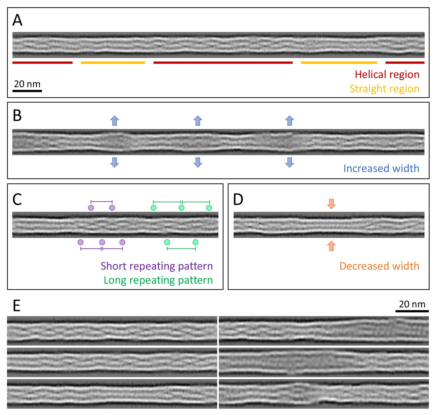
Computationally reconstituted filaments provide a realistic view of the KIFs at higher resolution (see Materials and methods). (A – D) Scale bar: 20 nm. (A) A typical keratin filament consisting of various regions with helical and straight-line patterns, indicated by red and yellow lines, respectively. (B) Keratin filament displaying diameter fluctuations. Areas of increased diameter are indicated (blue arrows). (C) Keratin filament showing helical patterns exhibiting different pitches, indicating modulations within the ice layer. Short repeating patterns (purple) indicate higher tilt angles in comparison to longer repeating patterns of in-plane filament stretches (green). (D) Keratin filament displaying diameter fluctuations. Areas of decreased diameter are indicated (orange arrows). (E) A collage of six computationally reconstituted keratin filaments showing structural diversity (total n=4460 filaments).
Figure 3—figure supplement 1
Reconstitution of keratin filaments.
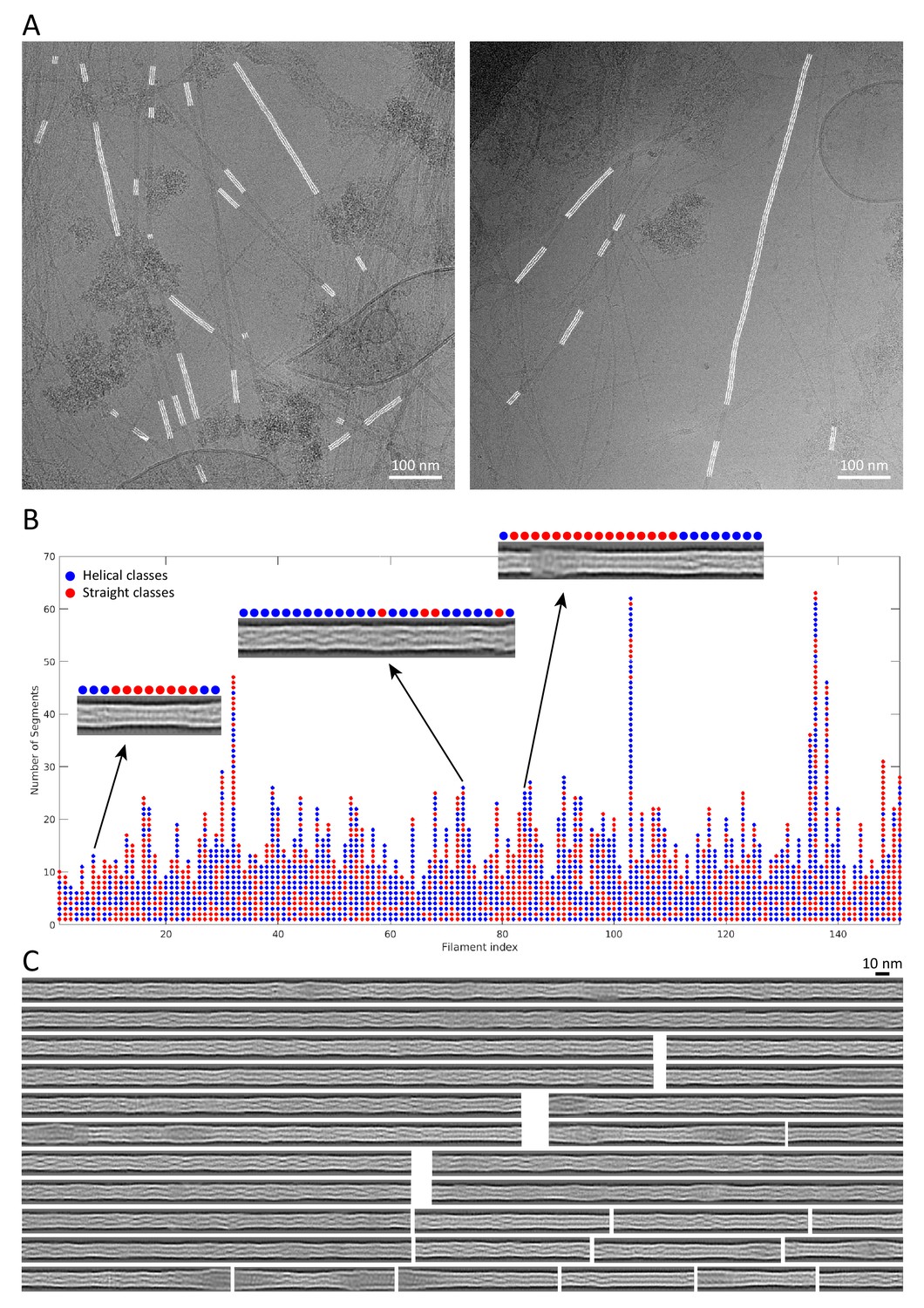
(A) Back-mapping of class averages onto the original filaments allowed us to assemble reconstituted, non-straightened keratin filaments in the original cryo-EM micrographs. Reconstituted filaments are displayed in white. (B) Keratin segments that originate from the same filament are plotted as columns of circles. The filaments are composed of helical (blue) and straight (red) class averages. Representative reconstituted filaments are shown and their composition by helical and straight classes is indicated. (C) Examples of reconstituted keratin filaments revealing the extensive heterogeneity in filament architecture.
Figure 4 with 1 supplement
Multiple protofilaments and an internal electron dense core are canonical components of keratin filaments.
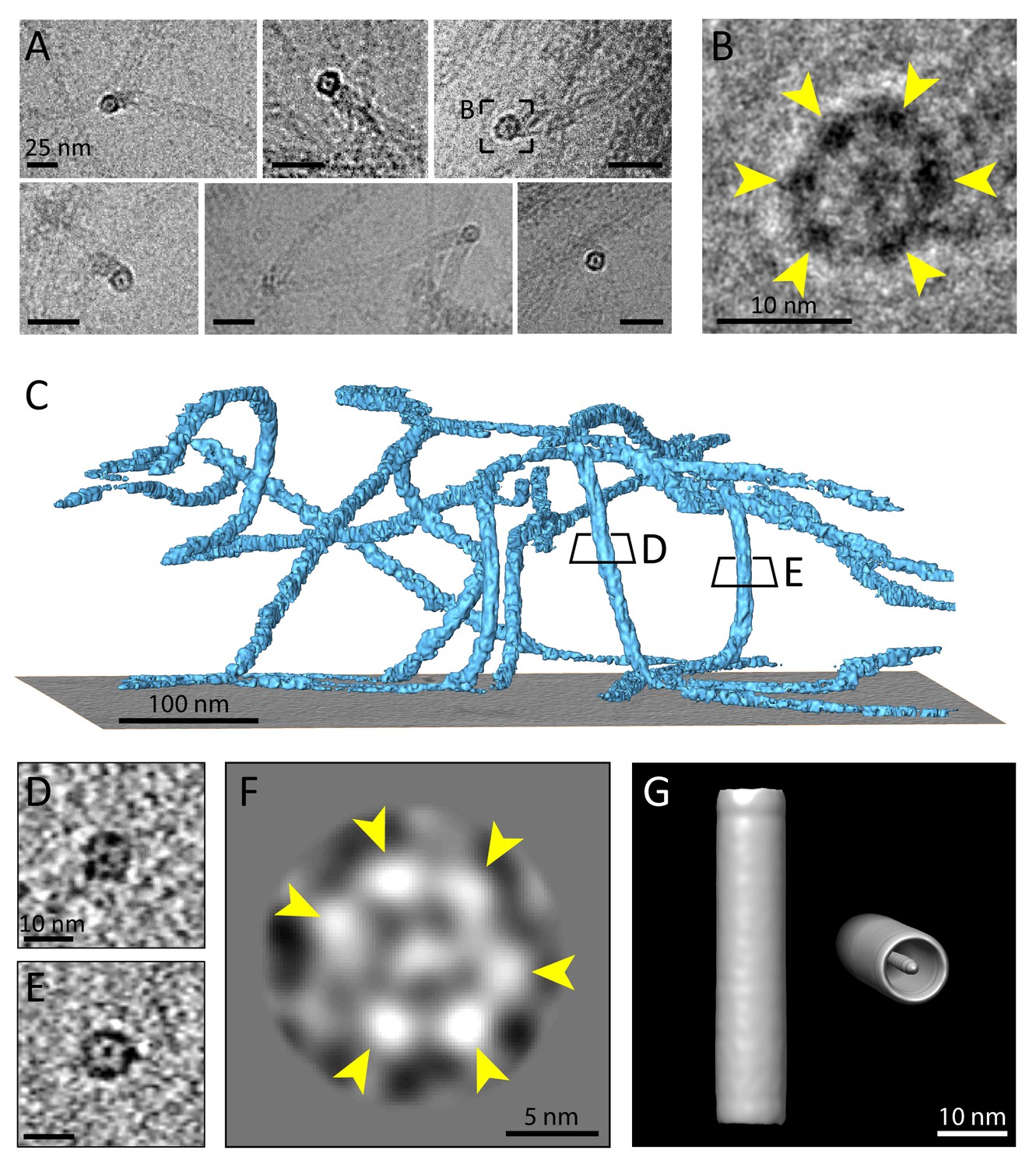
(A) Cross-section views of keratin filaments detected within the cryo-EM micrographs of ghost cells. An electron dense core is visible in the center of the keratin tube. Scale bars: 25 nm. (B) Zoomed-in view of the area boxed in (A). The cross section view reveals an internal core surrounded by six protofilaments as constituents of the tube (yellow arrowheads). (C) A surface rendered tomogram of a ghost cell was rotated in order to show the modulation of the keratin filaments within the ice layer (n=44). The three-dimensional keratin network is visualized (light blue). The level of the support is shown as a gray colored slice. Tomographic slices through vertically oriented filaments showing cross section views are indicated by boxes. (D) - (E) 7 nm thick xy-slices of the areas indicated in (C), showing KIFs as tube-like structures with a central density. Individual protofilaments can be identified. Scale bars: 10 nm. (F) A 2D class average of cross-section views extracted from individual regions of vertically oriented filaments (n=19), revealing the six individual protofilaments constituting the keratin filament tube (yellow arrowheads). (G) Low-resolution 3D model indicating the overall dimensions of a keratin filament and the presence of the central density. The structure was calculated template-free by randomizing the rotation angle of extracted 55 nm long keratin segments. Left: Side view. Right: Tilted cross section view revealing internal electron dense core.
Figure 4—figure supplement 1
Keratin filaments show a unique flexibility and contain a central density.
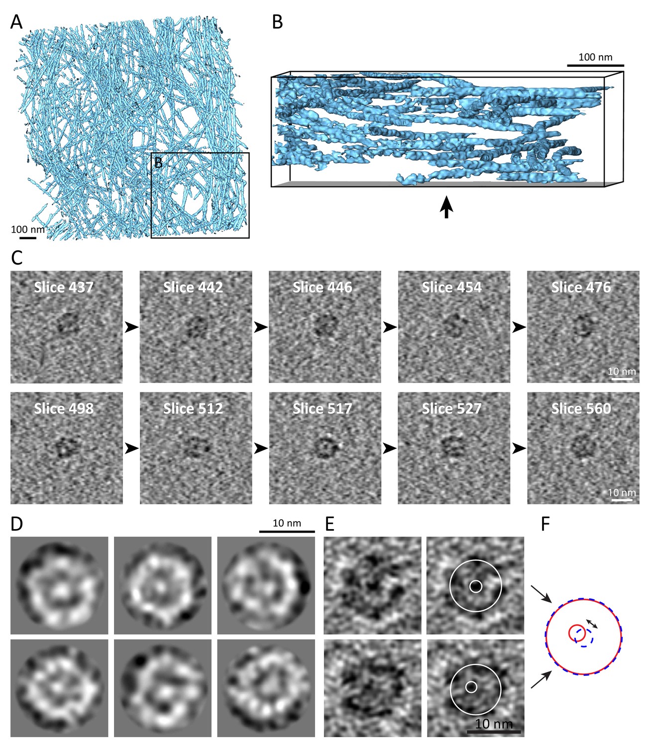
(A) Surface rendering of a tomogram of the vimentin network (blue) in a mouse embryonic fibroblast (MEF) ghost cell. The vimentin network shows reduced flexibility in comparison to keratin filaments, as vimentin filaments span less through the height of the tomographic volume. No cross-section views could be detected in 225 vimentin tomograms that were acquired. (B) Rotated view of the area boxed in (A), showing a side view of the vimentin network that reveals less fluctuations through the height of the tomogram volume when compared to keratin filaments (Figure 4C), although the tomograms have a comparable thickness. The arrow indicates the viewing direction from (A). (C) Sequential 7 nm thick xy-slices through two sub-tomograms containing single keratin filaments in cross section views. The top and the bottom row show different filaments. Cutting through these filaments emphasizes the variable appearances detected in different slices and allow the identification of more or less protofilaments, respectively. All slices reveal the internal electron dense core. Scale bars: 10 nm. (D) 2D class averages of CTF-corrected keratin filament cross-section views. Individual protofilaments in the ring and an electron dense core can be identified. (E) Two cross section views, representing 4.2-nm-thick slices along a single filament. The keratin filament (labeled with E in Figure 4D) was rotated in silico to a precise cross section orientation and projection images were calculated. On the right, the filament tube and the position of the central density are marked by white circles. (F) Schematic representation of the filament tube and the position of the central density in the filament cross-sections seen in (E). While in the upper panel of (E) the central density lies precisely in the center of the tube (red circles), in the lower panel of (E) the central density is shifted toward one side of the filament (blue dashed circles). The shift is evident in the overlay (double arrow).
Videos
Video 1
Cryo-tomogram of a keratin network in a ghost cell.
Video 2
Cryo-tomogram showing the modulations of the keratin filaments within the ice layer.
Tables
Key resources table
| Reagent type (species) or resource | Designation | Source or reference | Identifiers | Additional information |
|---|---|---|---|---|
| Gene (Mus musculus) | Krt6a | UniProtKB - P50446 | Targeted by CRISPR/Cas9 Knockout | |
| Gene (Mus musculus) | Krt6b | UniProtKB - Q9Z331 | Targeted by CRISPR/Cas9 Knockout | |
| Strain, strain background (E. coli) | DH5α | ThermoFisher Scientific | Cat# 18265017 | Chemically competent cells |
| Cell line (Mus musculus) | KtyI KO K14 | Homberg et al., 2015. DOI: 10.1038/jid.2015.184 | T. Magin lab, Institute of Biology, University of Leipzig, Germany. Cell line used to generate K5/K14_1 cell line | |
| Cell line (Mus musculus) | K5/K14_1 | This paper | Clonal knockout cell line of Krt6a and Krt6b, maintained in the Medalia lab | |
| Antibody | Anti-mouse Keratin 14 (mouse monoclonal) | ThermoFisher Scientific | MA5-11599, Clone LL002 | (1:100 – 1:10) |
| Antibody | Anti-mouse Keratin 5 (rabbit polyclonal) | BioLegend | Cat# 905503 | (1:500) |
| Antibody | Anti-mouse Keratin 6a (rabbit polyclonal) | BioLegend | Cat# 905702 | (1:500) |
| Antibody | Cy3 AffiniPure anti-rabbit (donkey polyclonal) | Jackson Immuno Research | Cat# 711-165-152 | (1:100) |
| Antibody | FITC AffiniPure anti-mouse (donkey polyclonal) | Jackson Immuno Research | Cat# 715-095-150 | (1:100) |
| Recombinant DNA reagent | pX458 (pSpCas9(BB)−2A-GFP) (plasmid) | Addgene | Cat# 48138 | CRISPR/Cas9 knockout |
| Recombinant DNA reagent | pGEM-T Easy (plasmid) | Promega | Cat# A1360 | |
| Sequence-based reagent | guideRNA insert targetting Krt6a and Krt6b gene | This paper | guideRNA sequence: GAGCCACCGCTGCCCCGGGAG. guideRNA cloned into pX458 plasmid and transfected into KtyI KO K14 cells. | |
| Commercial assay or kit | P3 primary cell 4D-Nucleofector kit | Lonza | Cat# V4XP-3032 | Transfection of KtyI KO K14 cells |
| Commercial assay or kit | jetPRIME | Polyplus transfection | Cat# 114–07 | Transfection of KtyI KO K14 cells |
| Commercial assay or kit | GenElute Mammalian Genomic DNA kit | Sigma-Aldrich | Cat# G1N70-1KT | Genomic DNA extraction |
| Chemical compound, drug | 99.9% anhydrous methanol | Alfa Aesar | Cat# 41838 | Fixation of mammalian cells |
| Chemical compound, drug | Hoechst 33342 | Sigma-Aldrich | Cat# B2261 | (1:10000) |
| Chemical compound, drug | Dako mounting medium | Agilent | Cat# S3023 | |
| Chemical compound, drug | Prolong Glass Anti-Fade | ThermoFisher Scientific | Cat# P36980 | |
| Software, algorithm | TIDE webtool | Netherlands Cancer Institute | https://tide.nki.nl/ | CRISPR/Cas9 knockout analysis |
| Software, algorithm | FIJI | Max Planck Institute of Molecular Cell Biology and Genetics, Dresden, Germany | RRID:SCR_002285 | For data analysis |
| Software, algorithm | Illustrator | Adobe Inc | RRID:SCR_010279 | For data analysis |
| Software, algorithm | OriginPro | OriginLab | RRID:SCR_014212 | For data analysis |
| Software, algorithm | MATLAB | MathWorks | RRID:SCR_001622 | For data analysis |
| Software, algorithm | RELION | Scheres, 2012. DOI: 10.1016/j.jsb.2012.09.006 | RRID:SCR_016274 | For data analysis |
| Software, algorithm | IMOD | University of Colorado Boulder, Colorado, USA | RRID:SCR_003297 | For data analysis |
| Software, algorithm | Amira | ThermoFisher Scientific | RRID:SCR_007353 | For data analysis |
| Software, algorithm | SerialEM | University of Colorado Boulder, Colorado, USA | RRID:SCR_017293 | For data acquisition |
| Software, algorithm | UCSF Chimera | University of California, California, USA | RRID:SCR_004097 | For structure visualization |
Additional files
Download links
A two-part list of links to download the article, or parts of the article, in various formats.
Downloads (link to download the article as PDF)
Open citations (links to open the citations from this article in various online reference manager services)
Cite this article (links to download the citations from this article in formats compatible with various reference manager tools)
Structural heterogeneity of cellular K5/K14 filaments as revealed by cryo-electron microscopy
eLife 10:e70307.
https://doi.org/10.7554/eLife.70307


