Sensing complementary temporal features of odor signals enhances navigation of diverse turbulent plumes
- Department of Physics, Yale University, United States
- Department of Molecular, Cellular and Developmental Biology, Yale University, United States
- Quantitative Biology Institute, Yale University, United States
Figures
Figure 1
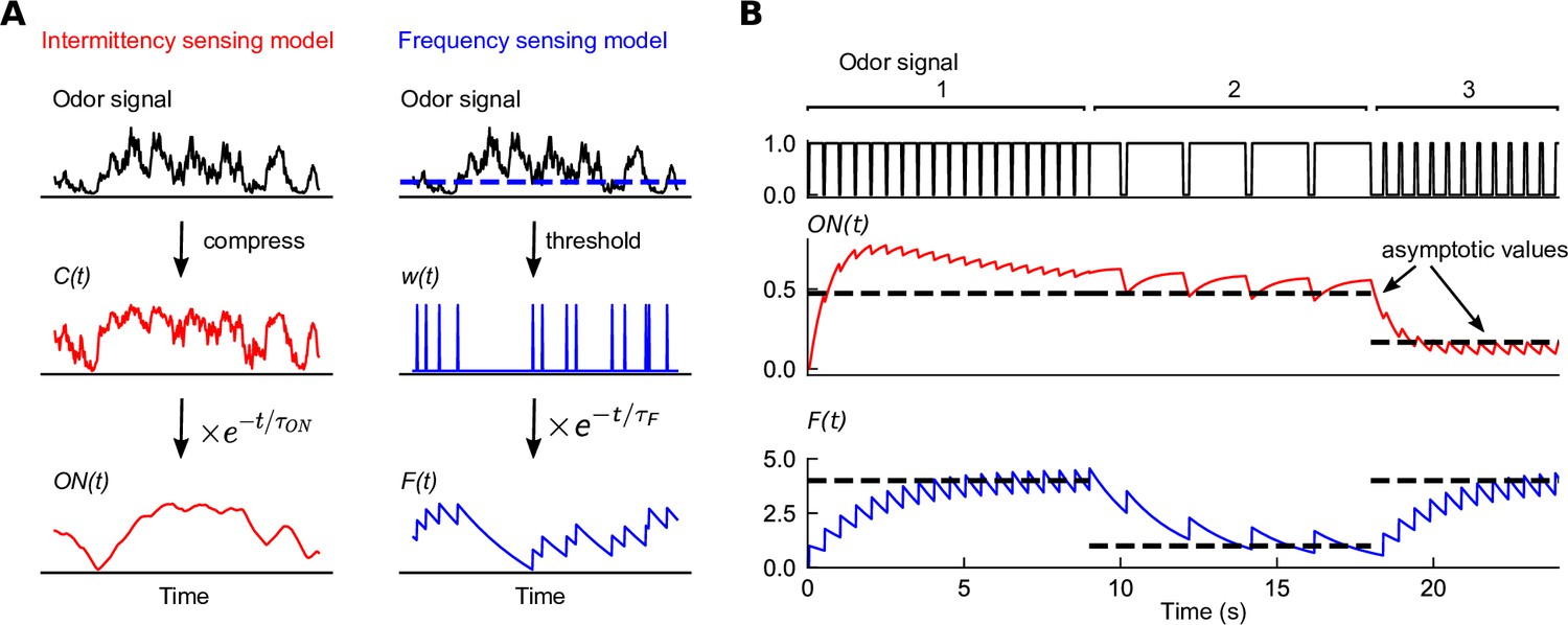
Filters extracted from experiment capture distinct temporal features of odor signals.
(A) Two experimentally informed models (Álvarez-Salvado et al., 2018; Demir et al., 2020) of Drosophila olfactory navigation transform odor signals in distinct ways. Left column: the intermittency model compresses the odor signal with an adaptive nonlinearity into a representation , bounded between 0 and 1. is then exponentially filtered with timescale to generate . Right column: the frequency model thresholds the odor signal (dashed line in top plot) into a binary representation , which is then passed through an exponential filter with timescale to generate . (B) Response of each of the models (bottom two plots) to a binary odor signal (top plot) of high intermittency, high frequency (region 1), high intermittency, low frequency (region 2), and low intermittency, high frequency (region 3). The intermittency model is sensitive to the intermittency of the signal – in regions 1 and 2, it approaches a high value asymptotically, but a low value when intermittency is low, even if the frequency remains high (region 3). The asymptotic values of the intermittency model (dashed lines) are , where I is signal intermittency (Materials and methods). Conversely, the frequency model exhibits sensitivity to the frequency of encounters, tending asymptotically towards , where is the signal frequency (dashed line). The frequencies in the three regions are 2 Hz, 0.5 Hz, and 2 Hz, the encounter durations are 0.45 s, 1.8 s, and 0.1 s, and the intermittencies are thus 0.9, 0.9, and 0.1.
Figure 2
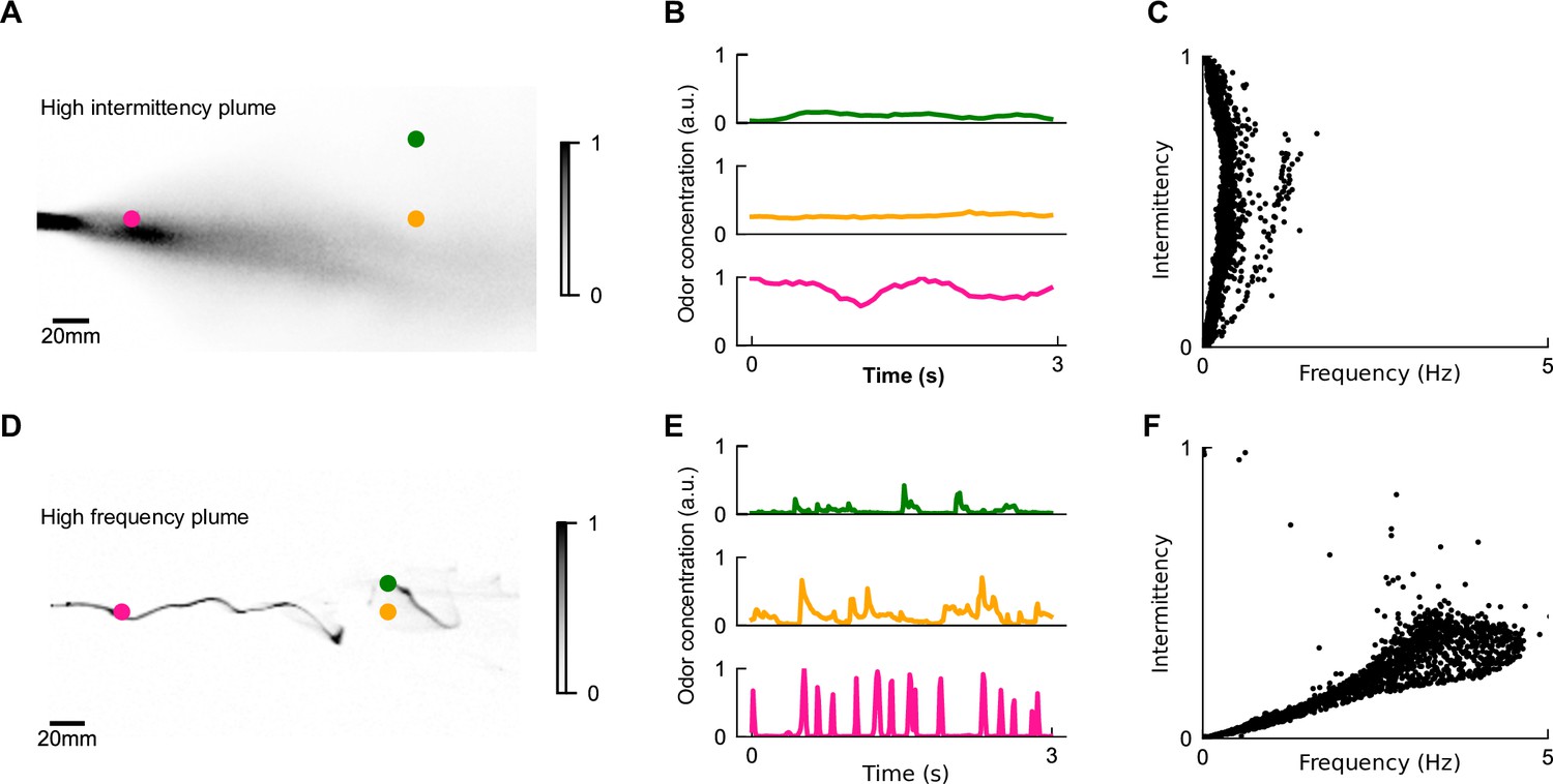
The differing temporal statistics of odor plumes.
(A) Snapshot of measured high-intermittency plume, reproduced from data in Connor et al., 2018. Colored dots: locations corresponding to odor series in (B). (B) Odor concentration time series at different locations in high-intermittency plume. (C) Intermittency versus whiff frequency for 10,000 uniformly distributed points in the high-intermittency plume. Statistics were calculated over the length of the full video. We see a range of intermittencies and many points with high intermittencies but relatively low frequencies. (D, E) High-frequency plume and representative time series, reproduced from data in Demir et al., 2020. (F) Analogous to (C) for the high-frequency plume. Data is clustered within a higher range of frequencies but low intermittencies.
Figure 3 with 1 supplement
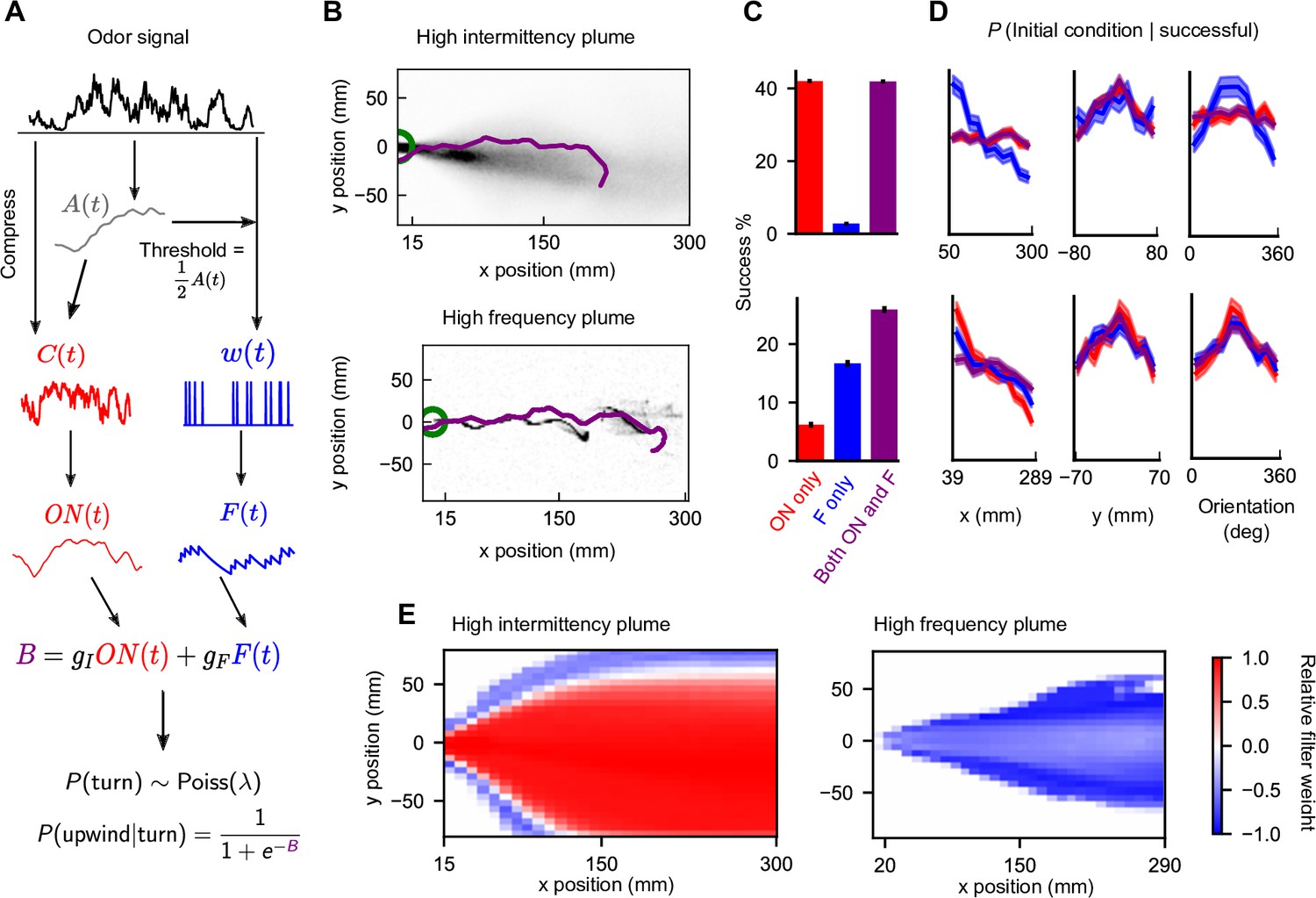
Sensing both intermittency and frequency enables navigation across diverse plumes.
(A) Our model linearly combines an intermittency sensor (red) and whiff frequency sensor (blue) to bias upwind motion. For both sensors, the odor signal is transformed using an adaptive compression step (Álvarez-Salvado et al., 2018) before being converted into a turning bias. Following (Demir et al., 2020), turns occur stochastically at a constant Poisson rate , while the sensor output B biases the likelihood that turns are upwind. Turn magnitudes are chosen from a normal distribution with mean 30° and SD 8° (Demir et al., 2020). (B) Example successful trajectories in the high-intermittency and high-frequency plume (Figure 2). (C) Percentage of agents that reach within 15 mm of the source when signal is present minus same percentage when signal is absent, for the model with only intermittency sensing (; red), only frequency sensing (; blue), or both ( nonzero; purple), in the high-intermittency plume (top) and high-frequency plume (bottom). Error bars: SEM calculated by bootstrapping the data 1000 times (Materials and methods). (D) Distribution of initial downwind position x (first column), crosswind position y (second column), and orientation (third column) for successful agents for the high-intermittency (top row) and high-frequency (bottom row) plumes. Colors correspond to same models as in (C). Upwind heading is 180°, and shaded regions represent SEMs obtained from bootstrapping (Materials and methods) (E) Time-averaged relative filter weight for different points in the two plumes.
Figure 3—figure supplement 1
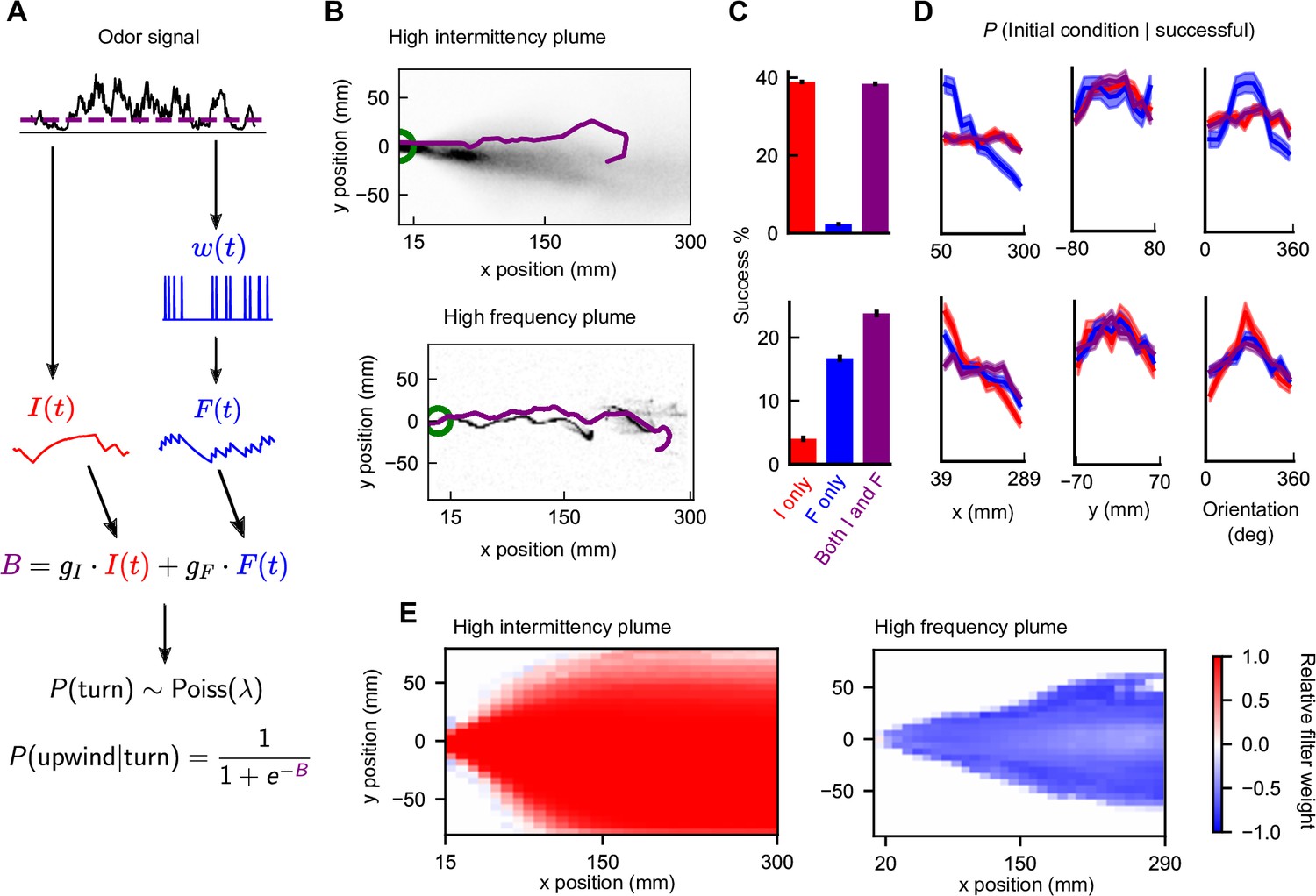
Fixed-threshold navigation model produces results similar to navigation model with adaptive intensity compression.
(A) The simplified model linearly combines a pure intermittency sensor (red) and whiff frequency sensor (blue) to bias upwind motion. Turns occur as above. (B) Example successful trajectories in the high-intermittency and high-frequency plume (see Figure 2). (C) Percentage of agents that reach within 15 mm of the source when signal is present minus same percentage when signal is absent, for the model with only intermittency sensing (; red), only frequency sensing (; blue), or both ( nonzero; purple), in the high-intermittency plume (top) and high-frequency plume (bottom). Error bars: SEM calculated by bootstrapping the data 1000 times (Materials and methods). (D) Distribution of initial downwind position x (first column), crosswind position y (second column), and orientation (third column) for successful agents for the high-intermittency (top row) and high-frequency (bottom row) plumes. Colors correspond to same models as in (D). Upwind heading is 180°, and shaded regions represent SEMs obtained from bootstrapping (Materials and methods). (E) Time-averaged relative filter weight for different points in the two plumes.
Figure 4 with 2 supplements
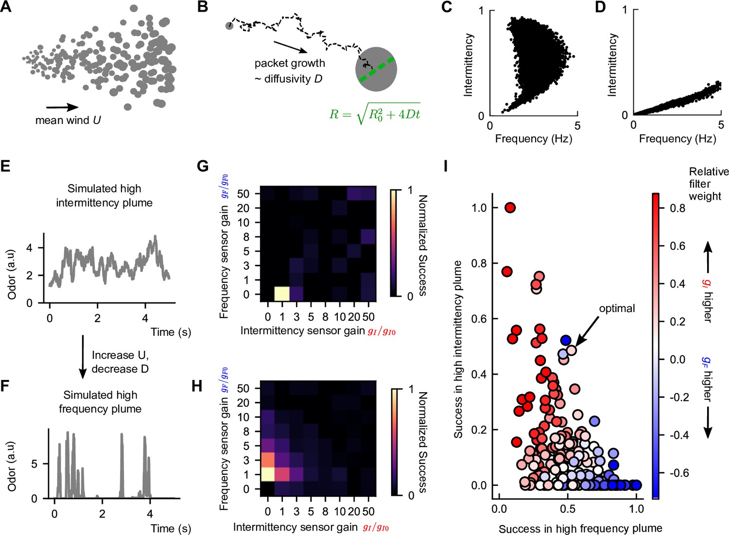
Performance trade-off between intermittency and frequency sensing in two diverse turbulent plumes.
(A) Example of a simulated odor plume, following the framework in Farrell et al., 2002. Gray circles denote Gaussian odor packets. (B) Example trajectory of a single-odor packet in these simulations and illustration of its growth. (C) Same as Figure 2C but for the simulated high-intermittency plume. (D) Same as (C) but for the simulated high-frequency plume. (E) Example odor concentration time series in a simulated high-intermittency plume. (F) Same as (C), for a high-frequency plume. (G) Normalized success percentage within the simulated high-intermittency plume after adding noise to I and F. is computed by first calculating the success percentage as in Figure 3C for each pair of gains and then normalizing by the maximum success percentage over all . Gains are measured in multiples of the base gains, defined in Materials and methods. (H) Same as (G), but for the simulated high-frequency plume. (I) in the simulated high-intermittency plume versus in the simulated high-frequency plume, where each dot represents a different . Points are colored by the relative weighting of the two sensors (see Materials and methods for calculation details). Note here that a finer set of gains was considered than in (G) and (H) and normalization was done with respect to these gains. The pair that maximized the geometric mean of normalized success percentage across the two plumes is indicated as optimal. The concavity of the front suggests a sharp trade-off in performance in one plume versus the other.
Figure 4—figure supplement 1
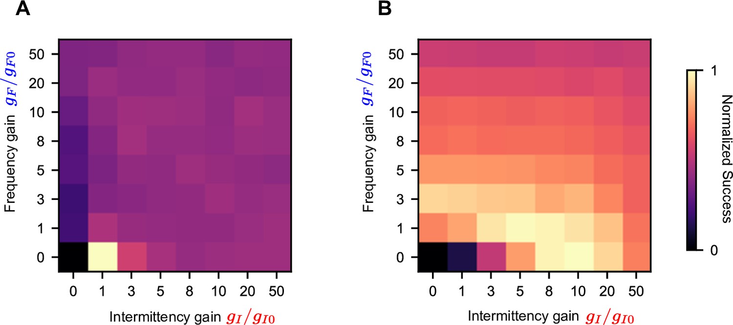
Performance of different sets of gains without filter noise.
Normalized success in the simulated high-intermittency plume (A) and simulated high-frequency plume (B) for different sets of and gains. We see strong performance in (B) for a large region at high-intermittency gains .
Figure 4—figure supplement 2
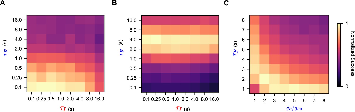
The effect of changing filter timescales on navigation success.
Normalized success in the simulated high-intermittency plume (A) and simulated high-frequency plume (B) for different values of and . Performance varies with and much more slowly with . (C) Normalized success in the simulated high-frequency plume for different values of and . Performance is roughly symmetric about , as expected.
Figure 5
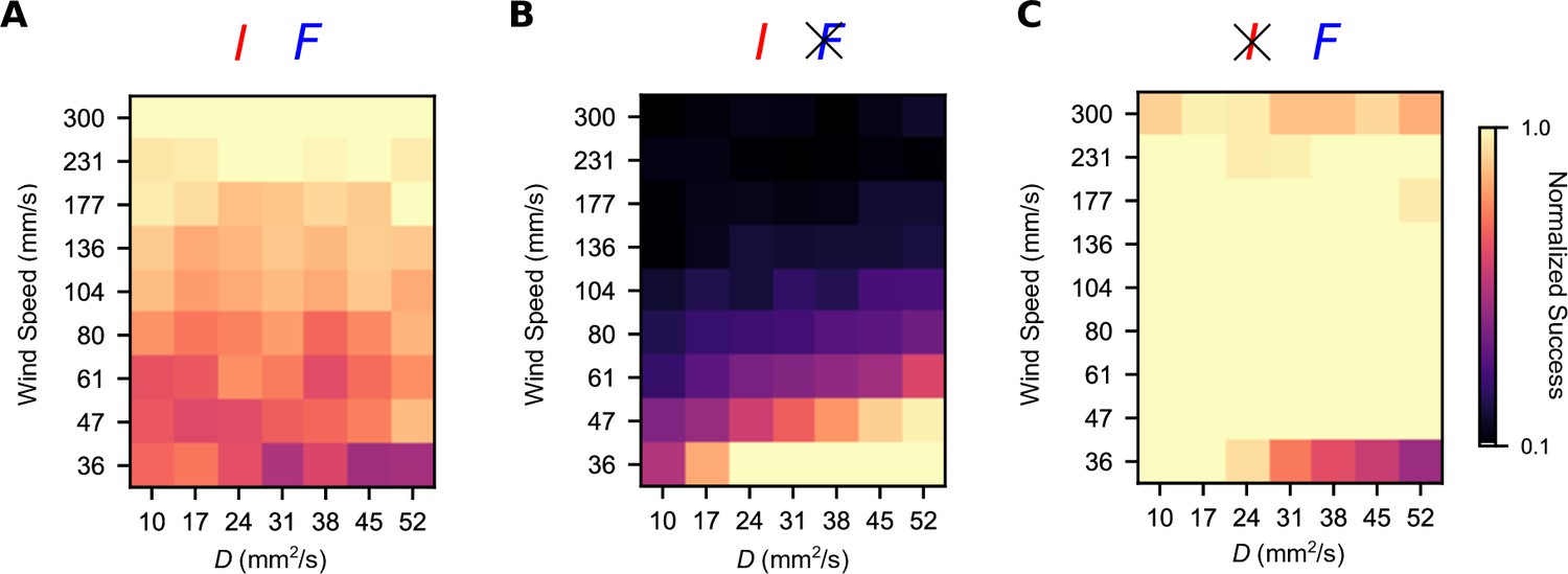
Simultaneous intermittency and frequency sensing maintains steady performance across a spectrum of odor environments, but does not allow for optimal performance.
Normalized success percentage for a frequency and intermittency-sensing model (A), only intermittency-sensing model (B), and only frequency-sensing model (C) for a range of simulated odor plumes. Success percentage is normalized such that the best performance of the three models is set to 1 for each environment. Gains for (A) were chosen to optimize the geometric mean of performance in the simulated high-intermittency and high-frequency plumes. Gains in (B) and (C) were chosen by taking the gains in (A) and then setting gF (A) and gI (C) to 0.
Figure 6
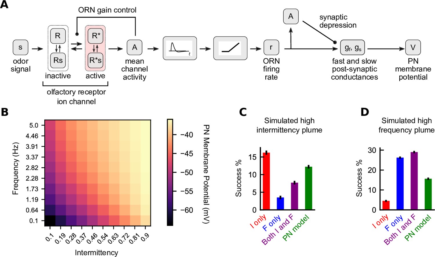
A biophysical signal transduction model allows for simultaneous frequency and intermittency sensing and performs similarly to a combined model.
(A) A schematic for how we combine the models of Gorur-Shandilya et al., 2017 and Nagel et al., 2015 to convert odor signals to projection neuron (PN) membrane potentials. (B) Time-averaged PN membrane potentials in square-wave environments of different frequency and intermittency. Responses were simulated for 30 s and last 20 s were averaged. (C) Performance of different navigation models considered in the simulated high-intermittency plume. Success was computed as in Figures 3 and 4. (D) Same as (C) but for the simulated high-frequency plume. Note that in (C) and (D) no noise was added to the filter outputs for any of the models.
Additional files
Download links
A two-part list of links to download the article, or parts of the article, in various formats.
Downloads (link to download the article as PDF)
Open citations (links to open the citations from this article in various online reference manager services)
Cite this article (links to download the citations from this article in formats compatible with various reference manager tools)
Sensing complementary temporal features of odor signals enhances navigation of diverse turbulent plumes
eLife 11:e72415.
https://doi.org/10.7554/eLife.72415


