Defining hierarchical protein interaction networks from spectral analysis of bacterial proteomes
- Department of Pathology and Immunology, Washington University School of Medicine, United States
- Duchossois Family Institute, University of Chicago, United States
- Department of Genetics, Washington University School of Medicine, United States
- Department of Developmental Biology, Washington University School of Medicine, United States
- The Edison Family Center for Genome Sciences and Systems Biology, Washington University School of Medicine, United States
- Department of Pathology, University of Chicago, Chicago, United States
- Center for the Physics of Evolving Systems, University of Chicago, Chicago, United States
Figures
Figure 1

Shallow components of covariation measured across bacterial orthologs reflect broad phylogenetic relationships.
(A) DOGG. Rows are 7047 bacterial proteomes, columns are 10,177 orthologous gene groups (OGGs), entries are the number of annotations of an OGG within a bacterial proteome (Figure 1—source data 1). (B) Percent variance explained versus spectral component (singular value decomposition [‘SVD] component’) number; fit is to a power-law distribution with the indicated exponent (γ). (C) Contributions of bacterial proteomes (colored dots) onto SVD components 1 through 4 (percent variance indicated in parenthesis on axis labels). Dots are colored according to phylum designation (color key).
-
Figure 1—source data 1
DOGG matrix shown in Figure 1A.
- https://cdn.elifesciences.org/articles/74104/elife-74104-fig1-data1-v2.zip
Figure 2 with 2 supplements

Workflow for relating patterns of ortholog covariation with phylogeny and protein interactions.
(A) Singular value decomposition (SVD) performed on DOGG yields UOGG (rows are proteomes, columns are ‘left singular vectors’ [LSVs]) and VOGG (columns are OGGs, rows are ‘right singular vectors’ [RSVs]). UOGG is used to relate information in the SVD spectrum with phylogenetic benchmarks. VOGG is used to relate information in the SVD spectrum with protein interaction benchmarks. (B,C) Spectral correlations between bacterial proteomes are calculated by defining spectral windows of five LSVs each (panel A) and computing correlated projections between proteomes across all spectral windows (panel B). (D,E) Spectral correlations between proteins within a proteome are calculated by (i) approximating the projections of proteins onto RSVs, (ii) defining spectral windows of five RSVs each (panel C), and (iii) computing correlated projections between proteins across all spectral windows (panel D). (F) The final step is to compute the information shared between spectral correlations and biological benchmarks of phylogenetic relationships (left panel) or protein interactions (right panel). Shown are example distributions of spectral correlations that have ‘high’ and ‘low’ amounts of MI with a benchmark.
Figure 2—figure supplement 1
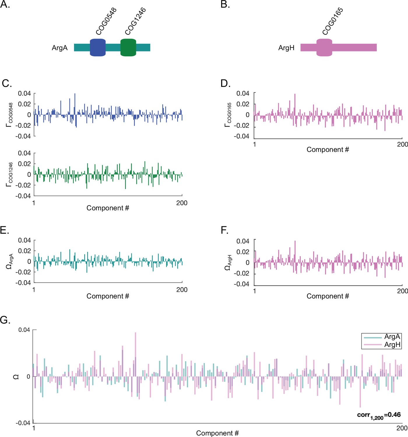
Computing spectral correlations between two proteins.
Shown here is an example of computing protein-protein spectral correlations using ArgA and ArgH in Escherichia coli K12. (A,B) The orthologous gene group (OGG) structures of E. coli K12 ArgA (panel A) and ArgH (panel B). (C,D) The projections () of the OGGs encoded in ArgA (COG0548 and COG1246) (panel C) and ArgH (COG0165) (panel D) onto SVD1 to SVD200 of the SVD (singular value decomposition) spectrum. (E,F) The approximated projections () of ArgA (panel E) and ArgH (panel F) derived by averaging the projections for the OGGs encoded within each protein. (G) Overlay of the approximated protein projections of ArgA and ArgH. These two proteins project similarly across SVD1 to SVD200 resulting in a positive spectral correlation value (Pearson correlation value shown).
Figure 2—figure supplement 2
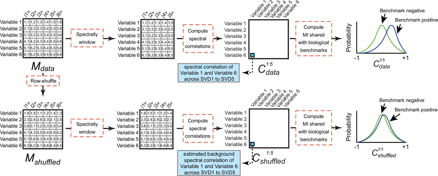
Computing background mutual information (MI) between spectral correlations and a benchmark.
(Top) Mdata consists of contributions of six variables (rows) onto six singular value decomposition (SVD) components (columns). If the variables correspond to the rows or columns of DOGG, the initial data matrix, Mdata corresponds to the UOGG or VOGG matrices produced by application of SVD to DOGG, respectively. Mdata is windowed to components 1–5. Next Pearson correlations are computed between all pairs of variables to produce the spectral correlation matrix Cdata1:5. The MI shared between Cdata1:5 and a benchmark reflects the degree to which the distribution of spectral correlation values in SVD1 to SVD5 differs for variable pairs that share the benchmark (‘Benchmark positive’) and variable pairs that do not share the benchmark (‘Benchmark negative’). (Bottom) To estimate the MI produced by spurious spectral correlations (i.e. ‘background MI’), Mdata is subjected to random row permutation to generate Mshuffled. This process maintains the distribution of spectral contributions for each variable but erases non-random spectral correlations leaving only random correlations produced by finite sampling. Mshuffled is subjected to the identical windowing, row correlation computation, and MI calculations as described above forMdata. We compute the biologically meaningful MI as the difference between the MI for Cdata1:5 and Cshuffled1:5.
Figure 3 with 1 supplement
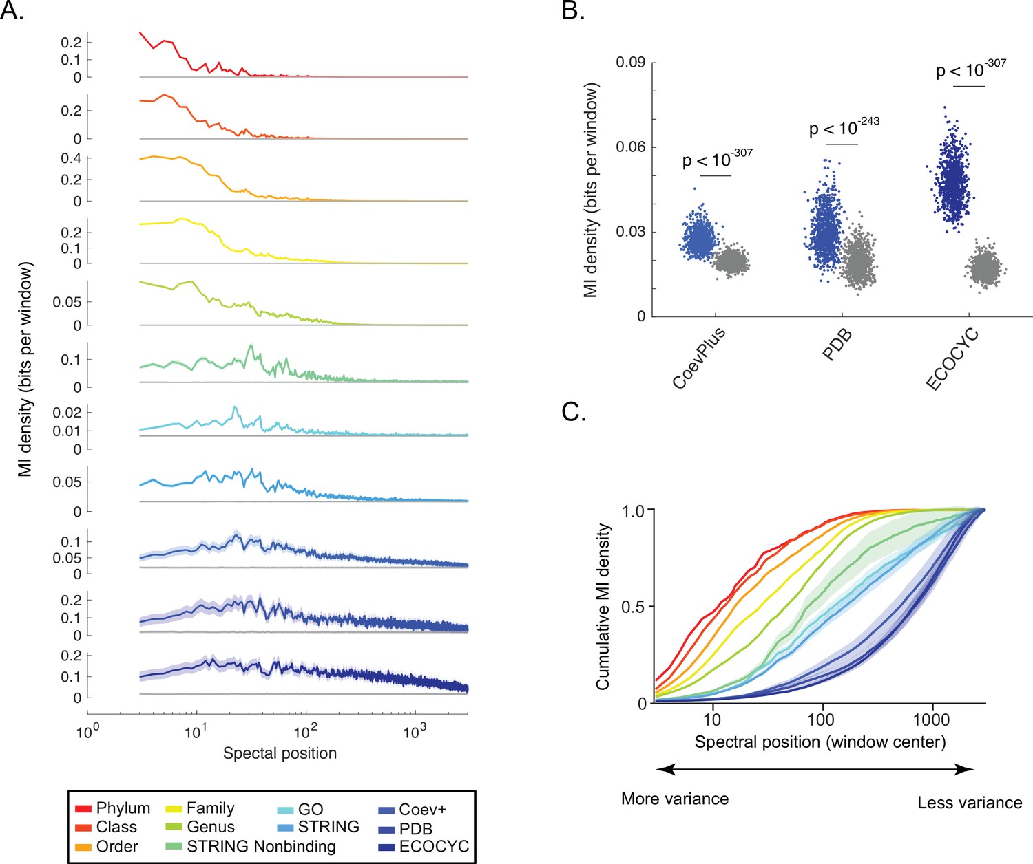
Shallow to deep spectral components of ortholog covariation reflect global to local biological ‘scales’.
(A) Distribution of information (y-axis, ‘mutual information [MI] density’) for each benchmark (see legend) measured across the singular value decomposition (SVD) spectrum (x-axis, ‘spectral position’). Gray line in each plot is the distribution of background MI (see Figure 2—figure supplement 2). Lines and shaded contours represent the mean±2 standard deviations for bootstraps of each benchmark. (B) Information shared between three benchmarks of direct protein-protein interactions (PPIs) (x-axis) and spectral correlations computed across SVD2996 to SVD3000. Each dot is the MI value for a single bootstrap of the indicated benchmark. Colored dots are non-random MI, gray dots are MI values for background spectral correlations. Values of statistical significance are shown above each distribution (p-value, Student’s t-test). (C) The degree to which information within the SVD spectrum reflects a biological benchmark, reported by the ‘cumulative density of MI’ (y-axis). As a curve for a benchmark approaches a value of ‘1’, deeper spectral components contain progressively less information regarding the benchmark. Colors follow those of panel A. Shaded regions are ±2 standard deviations of the mean MI value.
-
Figure 3—source data 1
NCBI taxonomic strings for each organism used to generate phylogenetic benchmarks.
- https://cdn.elifesciences.org/articles/74104/elife-74104-fig3-data1-v2.xlsx
-
Figure 3—source data 2
Benchmarks of protein-protein interactions (PPIs) in Escherichia coli K12.
- https://cdn.elifesciences.org/articles/74104/elife-74104-fig3-data2-v2.xlsx
Figure 3—figure supplement 1
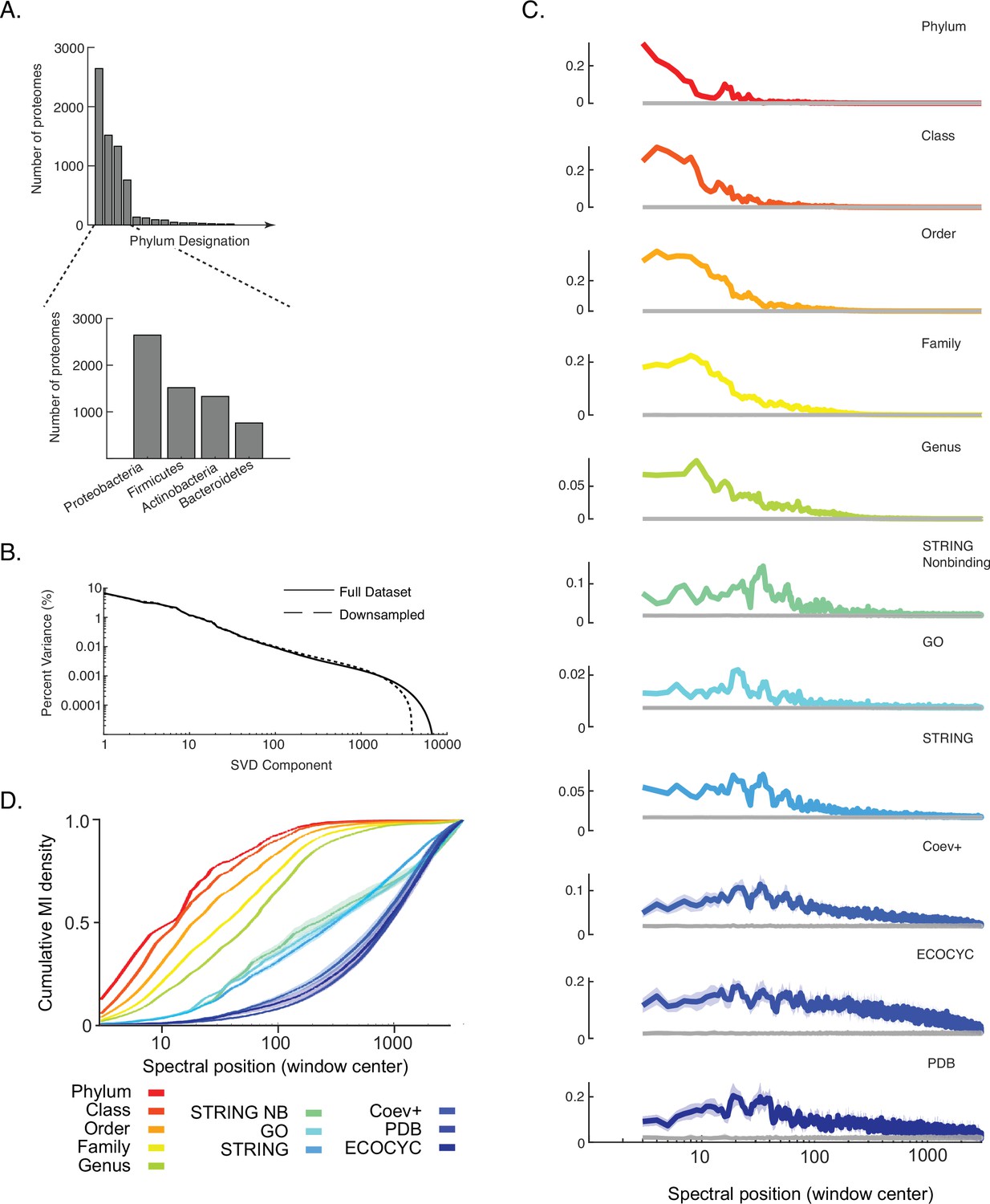
Impact of down-sampling overrepresented phyla on results shown in Figure 3.
(A) Histogram of the number of proteomes belonging to each of the top 15 out of a total 116 phyla in the data matrix DOGG. Inset is the four most abundant phyla. (B) Percent variance versus component number is plotted for the singular value decomposition (SVD) spectra of the initial data matrix DOGG and a ‘down-sampled’ version where the top four phyla were randomly subsampled to 50% their initial representation. (C) Distribution of information (y-axis, ‘cumulative MI density’) for each benchmark measured across the SVD spectrum of the down-sampled matrix (x-axis, ‘spectral position’). Gray line in each plot is the background MI. Lines and shaded contours represent mean ±2 standard deviations across 10 bootstraps of each benchmark. (D) Cumulative mutual information (MI) density for each benchmark across the SVD spectrum of the down-sampled matrix. Colors follow those of panel C. Lines and shaded contours represent mean ±2 standard deviations across 10 bootstraps of each benchmark.
Figure 4 with 1 supplement
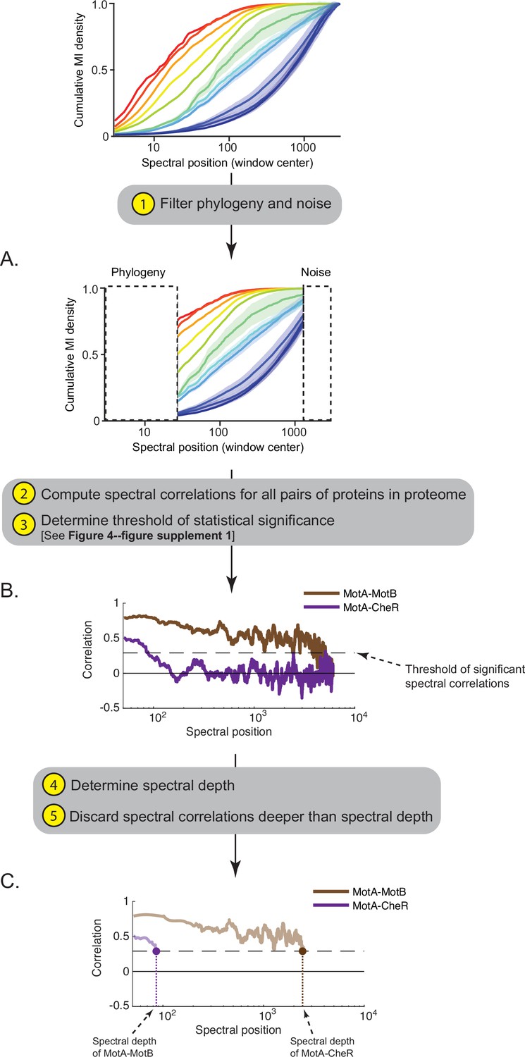
Workflow for computing the ‘spectral depth’ between pairs of proteins.
(A) Spectral components enriched for indirect and direct protein interactions (25th to 75th interquartile range of cumulative mutual information [MI] density) are selected, thereby filtering components enriched for phylogeny and noise. (B) Spectral correlations are computed for all pairs of proteins within a proteome; spurious spectral correlations introduced by finite sampling are filtered. Plotted here are spectral correlations (y-axis) as a function of spectral position (x-axis) for two pairs of proteins in Escherichia coli K12: MotA-MotB and MotA-CheR. Dashed line reflects the threshold defining statistically significant spectral correlations. (C) ‘Spectral depth’ is the spectral position at which the correlation value first reaches the threshold of statistical significance. Spectral depths of MotA-MotB and MotA-CheR are shown.
Figure 4—figure supplement 1
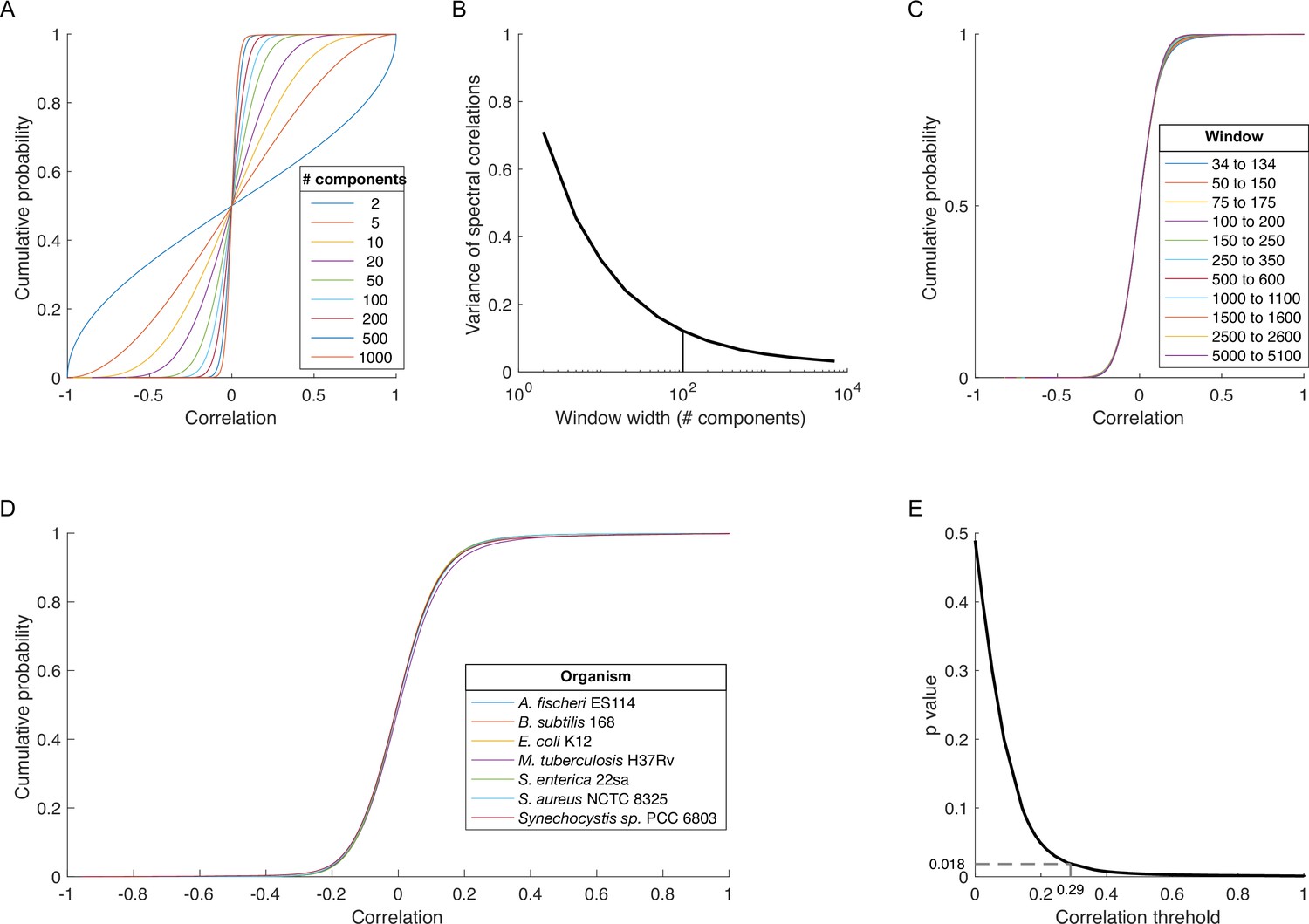
Determining a threshold for statistically significant spectral correlations.
(A) Cumulative distribution functions (cdfs) for spectral correlations between all proteins in Escherichia coli K12 across windows of different widths (legend) centered on SVD component 1001. (B) Variance of the distributions in panel A plotted versus window width. Vertical line indicates a window width of 100 components. (C) Cdfs for spectral correlations between all protein pairs in E. coli K12 across the different 100-component spectral windows (legend). (D) Cdfs for spectral correlations for all proteins in proteomes from diverse organisms (legend) across the 100-component window centered on SVD component 84. (E) p-Value versus correlation threshold for spectral correlations between proteins in E. coli K12 across components enriched for protein-protein interaction (PPI) information: SVD34 to SVD134. The chosen correlation threshold (0.29) is associated with a p-value of 0.018. SVD, singular value decomposition.
Figure 5
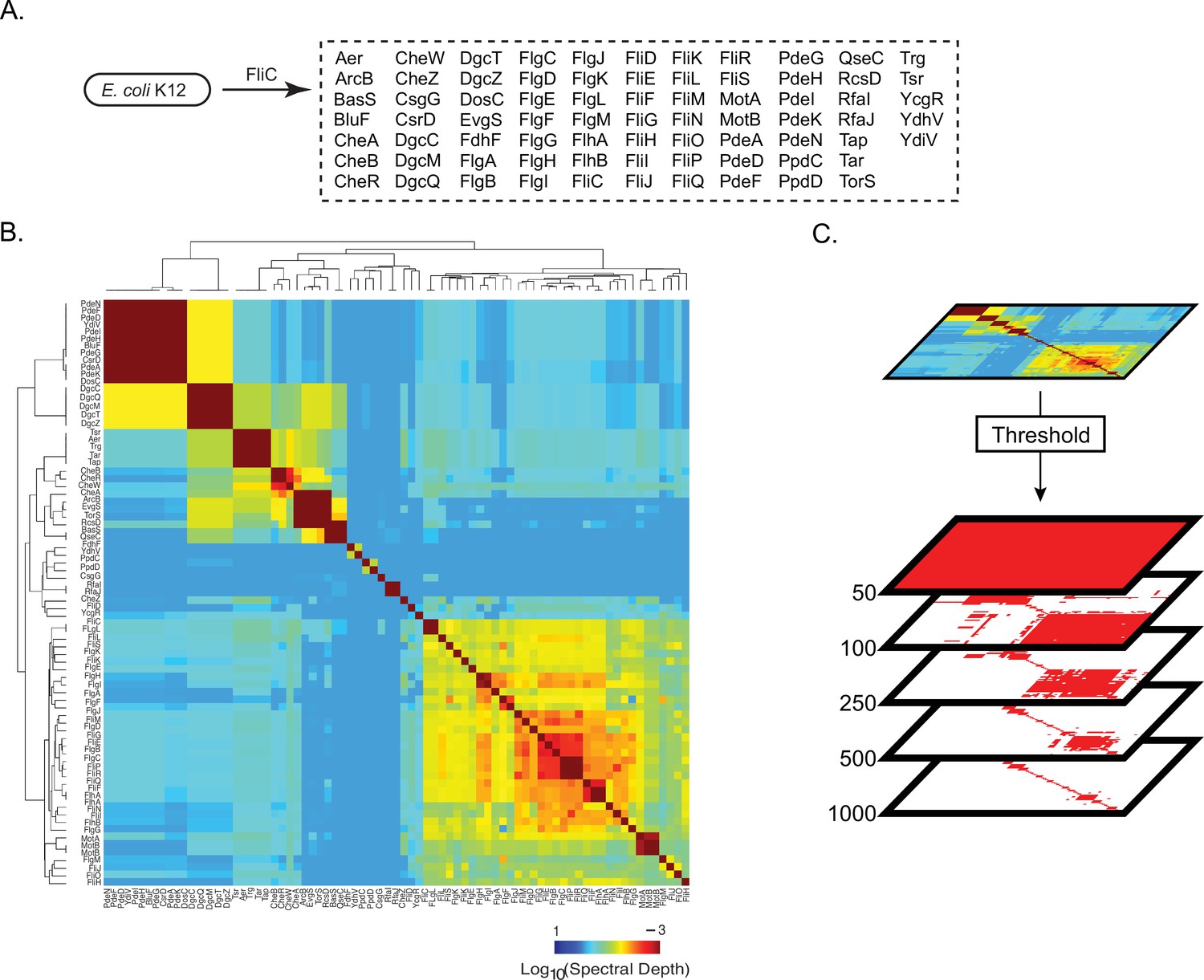
Pattern of spectral correlations with flagellar filament, FliC, in Escherichia coli K12.
(A) Proteins that shared significant spectral correlations with FliC after filtering for phylogeny and noise. (B) Hierarchically clustered spectral depth matrix for all pairs of proteins in panel A. (C) Set of matrices derived from thresholding the spectral depth matrix. Red pixels indicate that two proteins have a spectral depth deeper than the indicated threshold and therefore ‘statistically interact’. White pixels indicate that two proteins have a spectral depth of interaction shallower than the indicated threshold and therefore do not statistically interact.
Figure 6 with 4 supplements
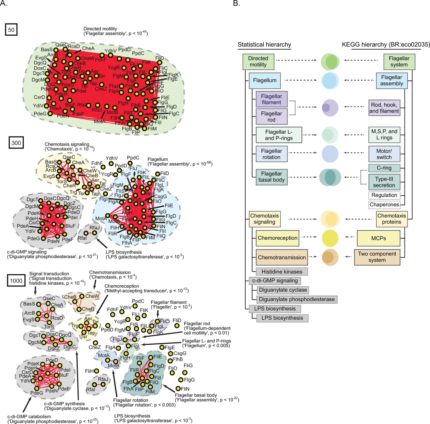
A statistically derived hierarchical model of Escherichia coli K12 motility.
(A) Statistical interaction networks defined at spectral depths 50 (top), 300 (middle), and 1000 (bottom). Nodes (yellow circles) are proteins; edges (red lines) reflect statistical interactions between proteins; contours are drawn around groups of connected proteins; assignment of function associated with contours is based on gene-set enrichment analysis (GSEA) with p-value of most-enriched GSEA term in parenthesis (Supplementary file 1). (B) Comparison of the statistically derived model (left) to the KEGG model (BR:eco02035, right) of E. coli K12 motility. Venn diagrams represent the overlap between the sets of proteins in the indicated subnetwork of panel A (left) and the indicated KEGG category (right).
Figure 6—figure supplement 1
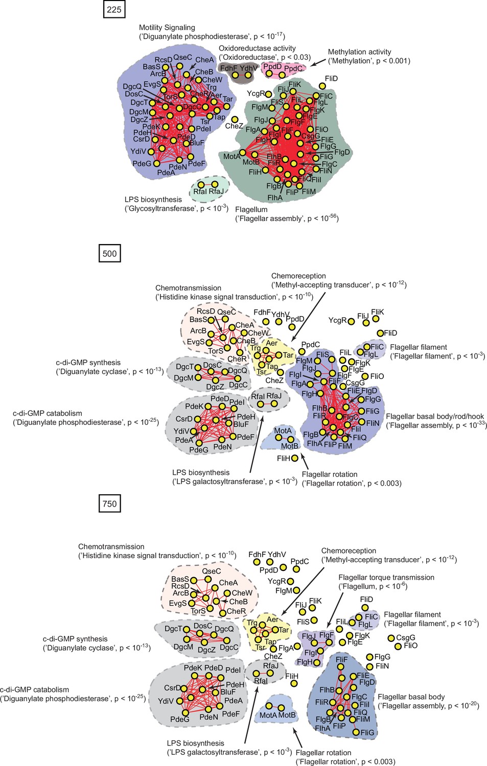
Protein interaction networks of spectrally correlated proteins with FliC in Escherichia coli K12 at spectral depths of 225, 500, and 750.
Nodes, edges, and contours are defined in the same manner as described in Figure 6A.
Figure 6—figure supplement 2
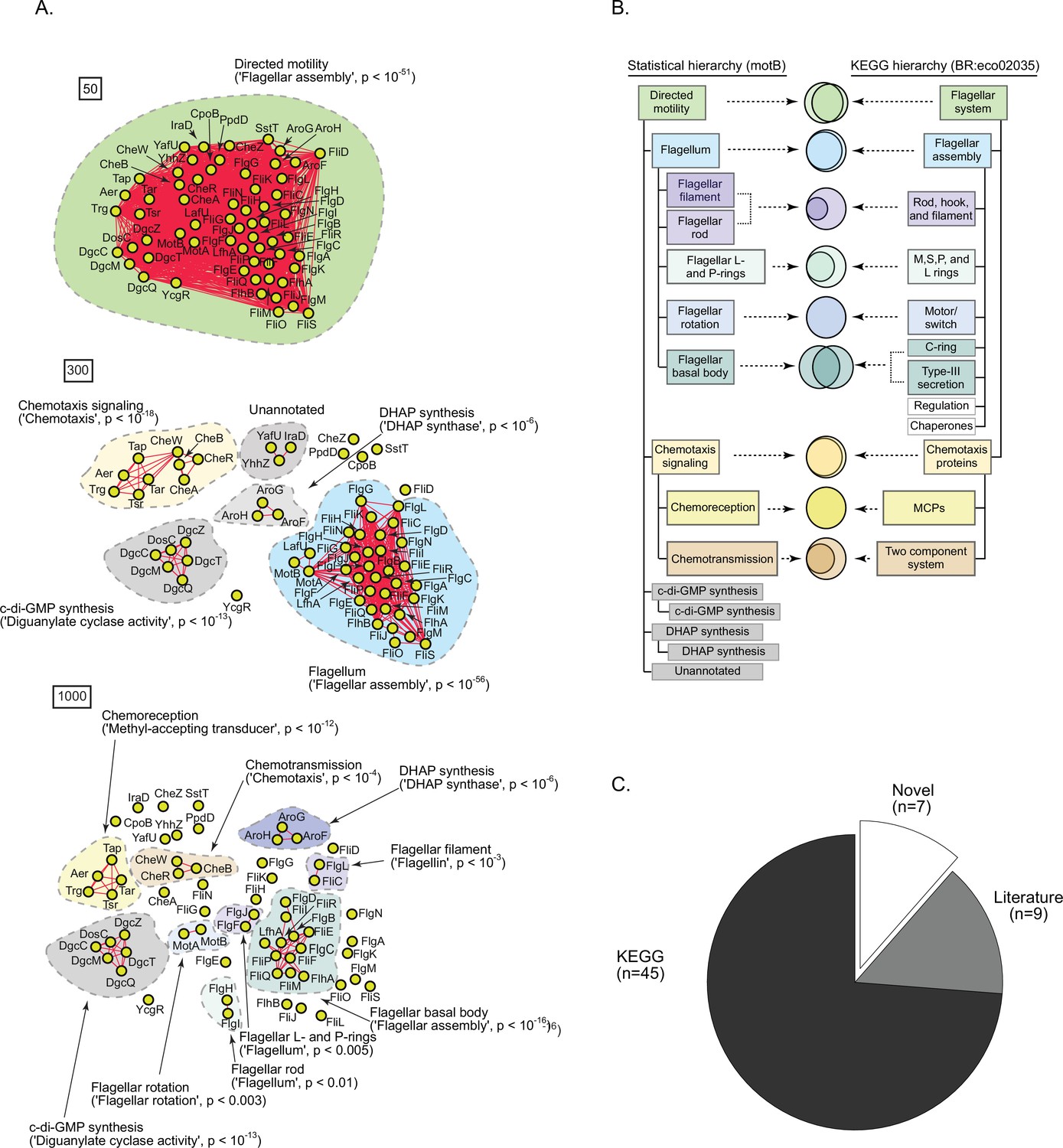
A statistically derived hierarchical model of motility in Escherichia coli K12 using MotB as a query protein.
(A) Statistical interaction networks defined by thresholding spectral depth at 50 (top panel), 300 (middle panel), and 1000 (bottom panel) (Supplementary file 2). Nodes, edges, and contours are defined in the same manner as described in Figure 6A. (B) Comparison of the statistically derived model using MotB (left) to the KEGG model (BR:eco02035, right) of E. coli K12 motility. (C) Number of statistically identified proteins found in KEGG, in existing literature, and putative novel effectors.
Figure 6—figure supplement 3
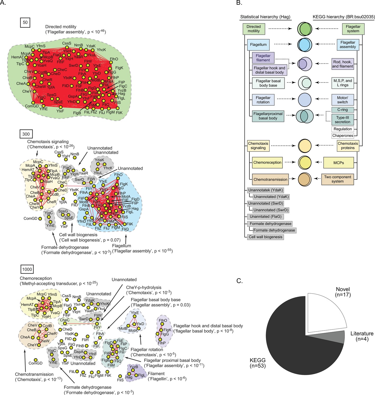
A statistically derived hierarchical model of motility in Bacillus subtilis 168 using Hag as a query protein.
(A) Statistical interaction networks defined by thresholding spectral depth at 50 (top panel), 300 (middle panel), and 1000 (bottom panel; Supplementary file 3). Nodes, edges, and contours are defined in the same manner as described in Figure 6A. (B) Comparison of the statistically derived model using Hag (left) to the KEGG model (BR:bsu02035, right) of B. subtilis 168 motility. (C) Number of statistically identified proteins found in KEGG, in existing literature, and putative novel effectors.
Figure 6—figure supplement 4
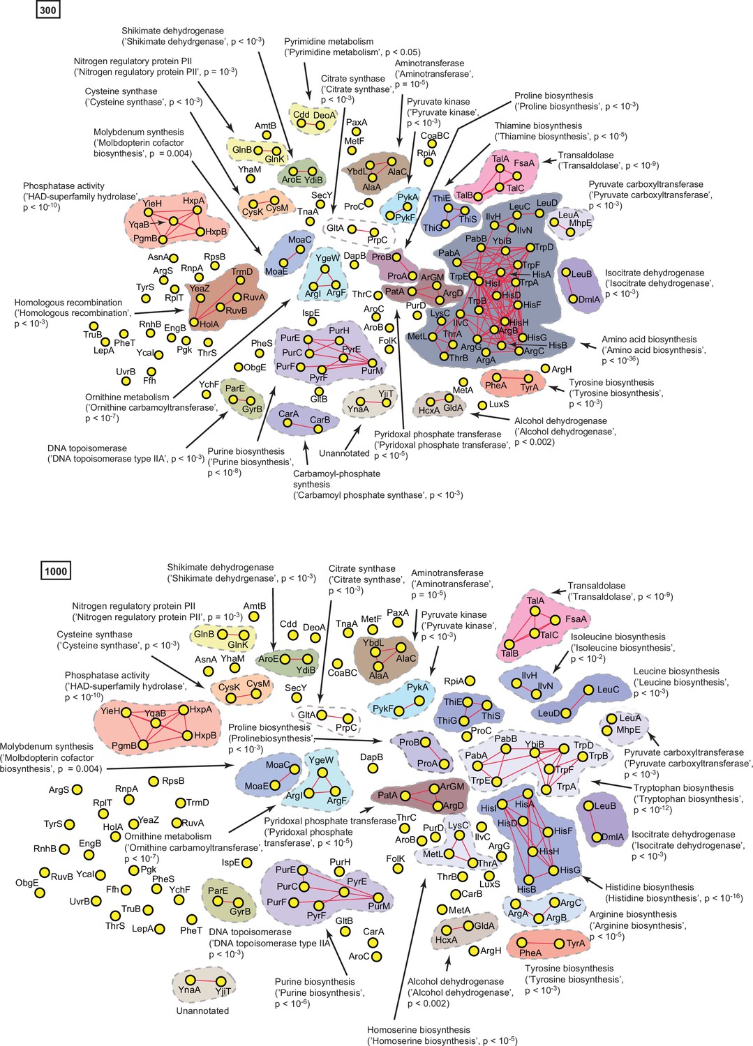
A statistically derived hierarchical model of amino acid metabolism in Escherichia coli K12 using HisG as a query protein.
(A) Statistical interaction networks defined by thresholding spectral depth at 300 and 1000. Nodes, edges, and contours are defined in the same manner as described in Figure 6—figure supplement 1, Supplementary file 4.
Figure 7 with 1 supplement
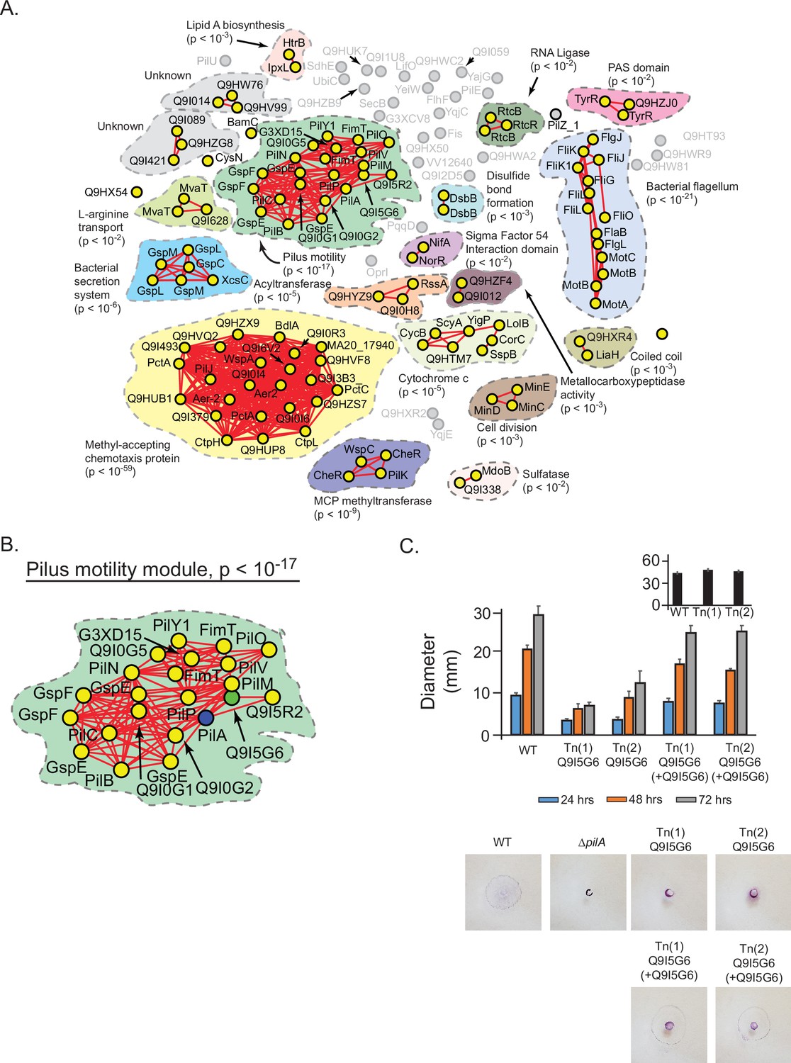
Prediction and validation of a novel effector of twitch motility in Pseudomonas aeruginosa.
(A) Statistical network derived by applying a spectral depth threshold of 300 to the set of 141 protein in P. aeruginosa (strain PAO1) that were significantly correlated with PilA across SVD34 to SVD134 (see Figure 7—figure supplement 1). Nodes, edges, shaded contours, gene-set enrichment analysis (GSEA) enrichment terms, and p-values are defined in the same manner as in Figure 6A. (B) The pilus motility subnetwork from panel A. Nodes representing PilA and Q9I5G6 are colored blue and green, respectively. (C) Time-course of pilus-based motility for parent (WT), two transposon mutants of Q9I5G6 (Tn(1) Q9I5G6, Tn(2) Q9I5G6), and transposon mutants complemented with Q9I5G6 (Tn(1) Q9I5G6+Q9I5G6, Tn(2) Q9I5G6+Q9I5G6). Inset shows results of flagellar motility for the parent strain (WT), and the two transposon mutants of Q9I5G6 (Tn(1), Tn(2)) 24 hr post-inoculation. Representative images of the crystal-violet stained plates are shown. SVD, singular value decomposition.
Figure 7—figure supplement 1
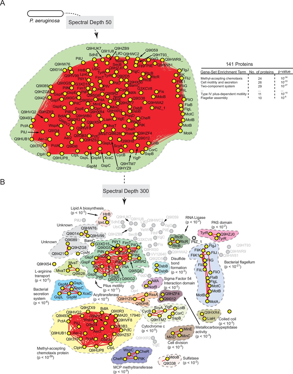
Statistically derived hierarchical model of directed motility in Pseudomonas aeruginosa using PilA as a query.
(A) Statistical interaction network defined by thresholding spectral depth at 50. The inset illustrates significantly enriched terms resulting from gene-set enrichment analysis (GSEA) of the entire network. (B) Statistical interaction network defined by thresholding spectral depth at 300 (Supplementary file 5). Nodes, edges, shaded contours, GSEA enrichment terms, and p-values are defined in the same manner as in Figure 6A.
Figure 8 with 3 supplements

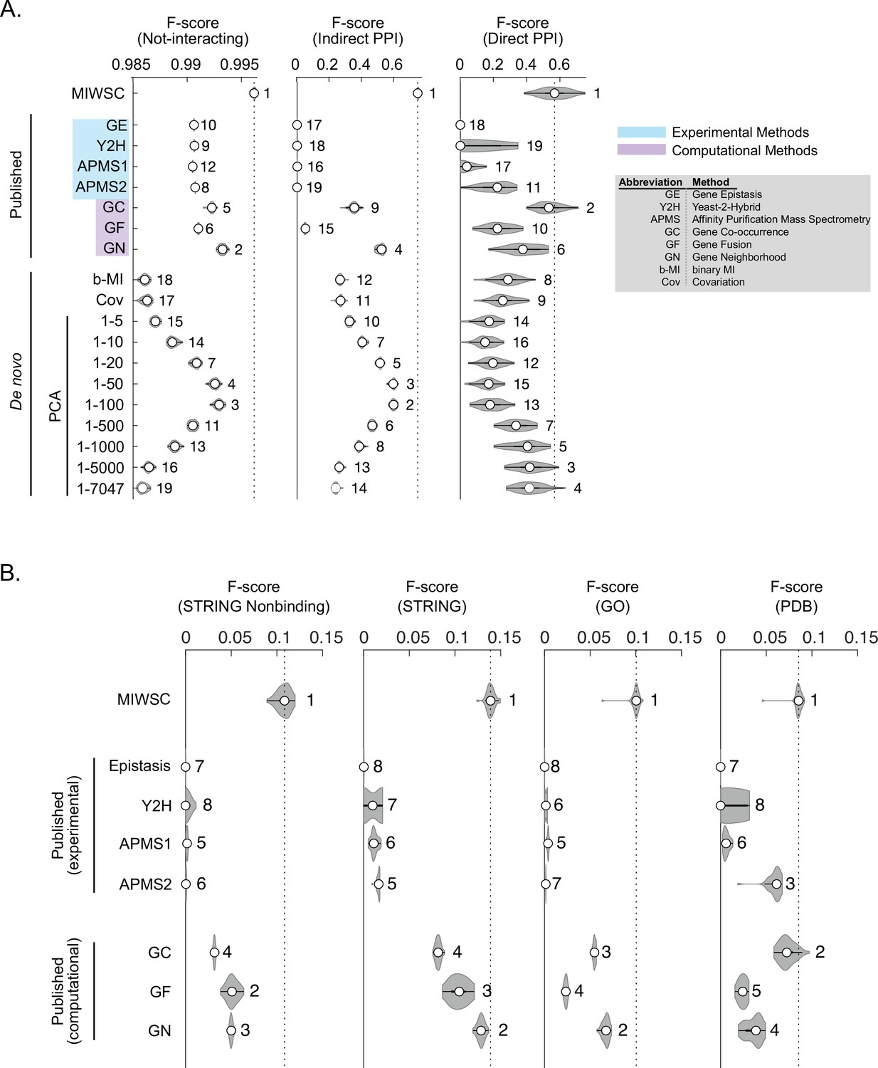
Mutual information (MI) windowed spectral correlations (MIWSCs) enable accurate classification of indirect and direct protein-protein interactions (PPIs).
See Figure 8—figure supplement 1 for definition of ‘MIWSCs’. (A) F-scores for predicting interaction classes for Escherichia coli K12 protein pairs using random forest (RF) models trained on MIWSCs or features from several different methods (see legend). Violin plots show distribution of F-scores for models trained and validated on 50 random partitions of the gold-standard dataset. Numbering indicates the rank of the median F-score for models trained on each feature (Figure 8—source data 1). (B) Precision (left) and recall (right) for predictions of any (indirect or direct), direct, or indirect PPIs in 12 bacteria using RF models trained on the MIWSCs of E. coli K12 proteins benchmarked against the experimentally supported PPIs in the STRING database (experimental score > 0). Comparisons are made to a set of 10,000 randomly selected pairs and to the ‘medium confidence’ predictions (score > 400) in the STRING database subchannels for GC, GN, and GF. Vertical dashed line indicates the median value for the best performing method. ** in legend indicates an organism that was not part of the input dataset DOGG (Figure 8—source data 1). (C) Precision-recall curves were constructed for the methods of GC, GN, GF by thresholding the subchannel scores at 150 (‘low confidence’), 400 (‘medium confidence’), 700 (‘high confidence’), and 900 (‘highest confidence’). The precision versus recall is plotted for any (indirect or direct), direct, or indirect PPIs predicted using the RF models trained on MIWSCs. Symbols and whiskers represent the median and 25–75 percentile range, respectively, for the predictions produced for the 12 organisms in panel B (Figure 8—source data 1). (D) Percent of predicted direct PPIs in Mycobacterium tuberculosis H37Rv supported by an absent (0), low (0–0.4), or high (>0.4) composite score (left) or an absent (0) or present (>0) experimental subchannel score (right) in the STRING database. Comparisons were made between the methods of random selection (Random), amino acid coevolution (Cong et al., 2019), or RF models trained on MIWSC features of E. coli K12 proteins (MIWSC). Numbers of predicted interactions in each bin are indicated (Figure 8—source data 1).
-
Figure 8—source data 1
Data and statistical support for random forest (RF) model validation studies, related to Figure 8Figure 8.
- https://cdn.elifesciences.org/articles/74104/elife-74104-fig8-data1-v2.xlsx
Figure 8—figure supplement 1
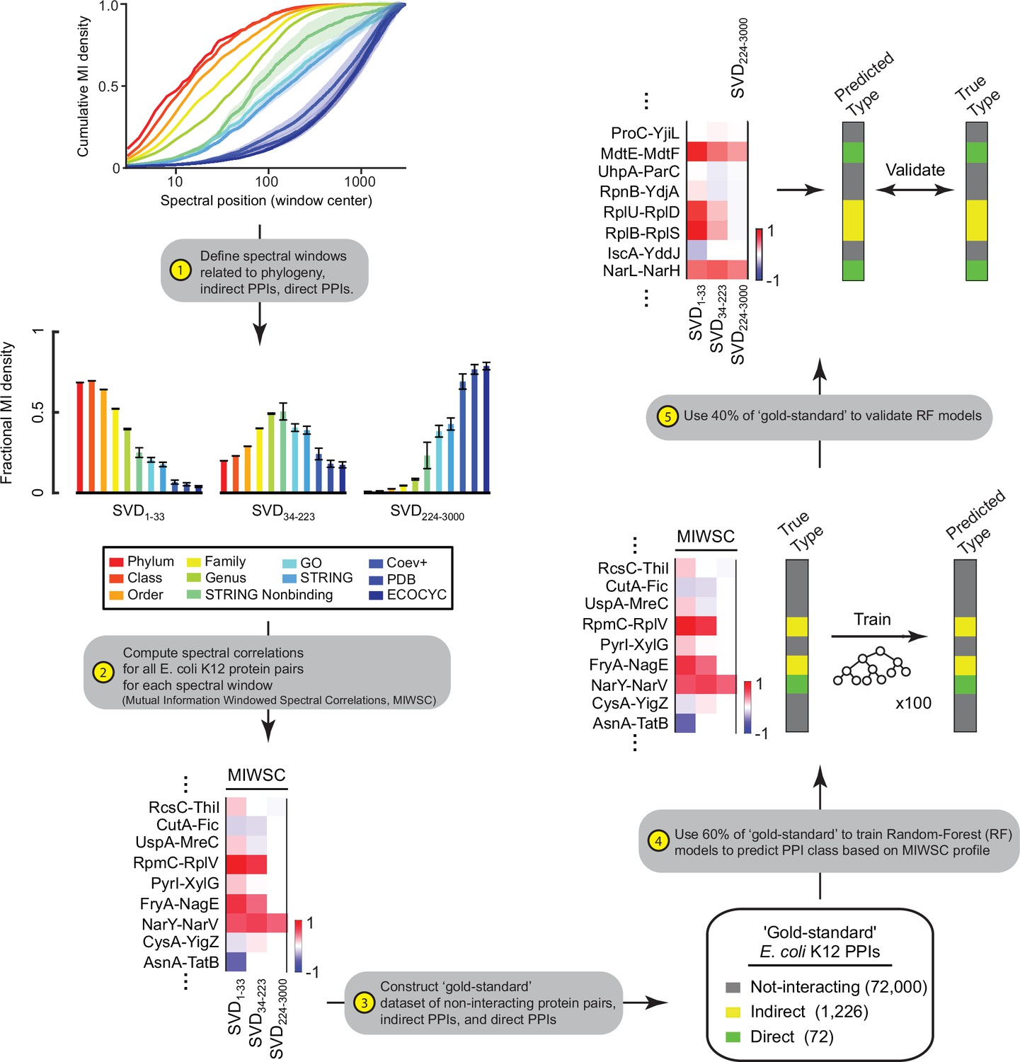
Workflow for training and validating random forest (RF) models on mutual information windowed spectral correlations (MIWSCs).
The five-step process described here yielded RF models trained to predict protein-protein interaction (PPI) class (either not-interacting, indirect PPIs, or direct PPIs) from the set of three MIWSC values.
Figure 8—figure supplement 2
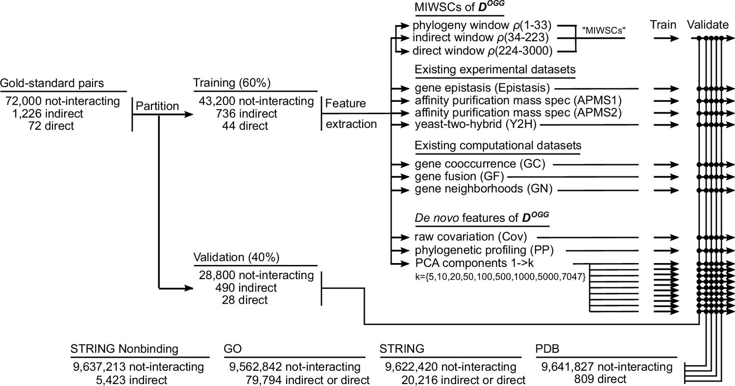
Workflow for training and validating various random forest (RF) models designed to predict non-interacting proteins, indirect protein-protein interactions (PPIs), and direct PPIs across the proteome of Escherichia coli K12.
A gold-standard dataset of well-characterized E. coli K12 protein pairs was assembled and partitioned into training and validation datasets. The labeled examples from the training set were used to train RF models to classify protein interactions. RF models were trained based on either mutual information windowed spectral correlations (MIWSCs), existing experimental features, existing computational features, or features derived from analysis of DOGG. The performance of the various RF models was benchmarked and compared by computing F-scores for classifying PPIs in the validation dataset, out-of-bag examples in the training dataset, and PPIs in four additional comprehensive benchmarks. This process of partitioning the gold-standard dataset, training, and validation was repeated 50 times to evaluate the reproducibility of RF model performance.
Figure 8—figure supplement 3
F-scores for predicting interaction classes for out-of-bag examples in the training datasets (A) and four additional comprehensive benchmarks (B).
The violin plots describe the distribution of F-scores for models trained and validated on 50 random partitions of the gold-standard dataset (Figure 8—figure supplement 1). Numbering indicates the rank of the median F-score for models trained on each feature (Figure 8—source data 1).
Additional files
-
Supplementary file 1
Data pertaining to Figure 6A.
- https://cdn.elifesciences.org/articles/74104/elife-74104-supp1-v2.xlsx
-
Supplementary file 2
Data related to Figure 6—figure supplement 2.
- https://cdn.elifesciences.org/articles/74104/elife-74104-supp2-v2.xlsx
-
Supplementary file 3
Data related to Figure 6—figure supplement 3.
- https://cdn.elifesciences.org/articles/74104/elife-74104-supp3-v2.xlsx
-
Supplementary file 4
Data related to Figure 6—figure supplement 4 .
- https://cdn.elifesciences.org/articles/74104/elife-74104-supp4-v2.xlsx
-
Supplementary file 5
Data related to Figure 7A,B and Figure 7—figure supplement 1.
- https://cdn.elifesciences.org/articles/74104/elife-74104-supp5-v2.xls
-
Supplementary file 6
Data related to gene co-occurrence, gene fusion, gene neighborhood, and co-expression data using pilA in Pseudomonas aeruginosa (PAO1) as a query protein.
- https://cdn.elifesciences.org/articles/74104/elife-74104-supp6-v2.xlsx
-
Supplementary file 7
Data related to Figure 7C.
- https://cdn.elifesciences.org/articles/74104/elife-74104-supp7-v2.xlsx
-
Transparent reporting form
- https://cdn.elifesciences.org/articles/74104/elife-74104-transrepform1-v2.docx
Download links
A two-part list of links to download the article, or parts of the article, in various formats.
Downloads (link to download the article as PDF)
Open citations (links to open the citations from this article in various online reference manager services)
Cite this article (links to download the citations from this article in formats compatible with various reference manager tools)
Defining hierarchical protein interaction networks from spectral analysis of bacterial proteomes
eLife 11:e74104.
https://doi.org/10.7554/eLife.74104


