Diversification dynamics in the Neotropics through time, clades, and biogeographic regions
- Institut des Sciences de l’Evolution de Montpellier (Université de Montpellier | CNRS | IRD | EPHE), Place Eugène Bataillon, France
- Real Jardín Botánico (RJB), CSIC, Spain
- Department of Anthropology, University of California, United States
- Mammal Section, The Natural History Museum, Cromwell Road, United Kingdom
- Institut Universitaire de France (IUF), France
- Royal Botanic Gardens, United Kingdom
- Ecology and Evolutionary Biology, University of Sheffield, United Kingdom
- Gothenburg Global Biodiversity Centre, Department of Biological and Environmental Sciences, University of Gothenburg, Sweden
- Department of Plant Sciences, University of Oxford, United Kingdom
Figures
Figure 1
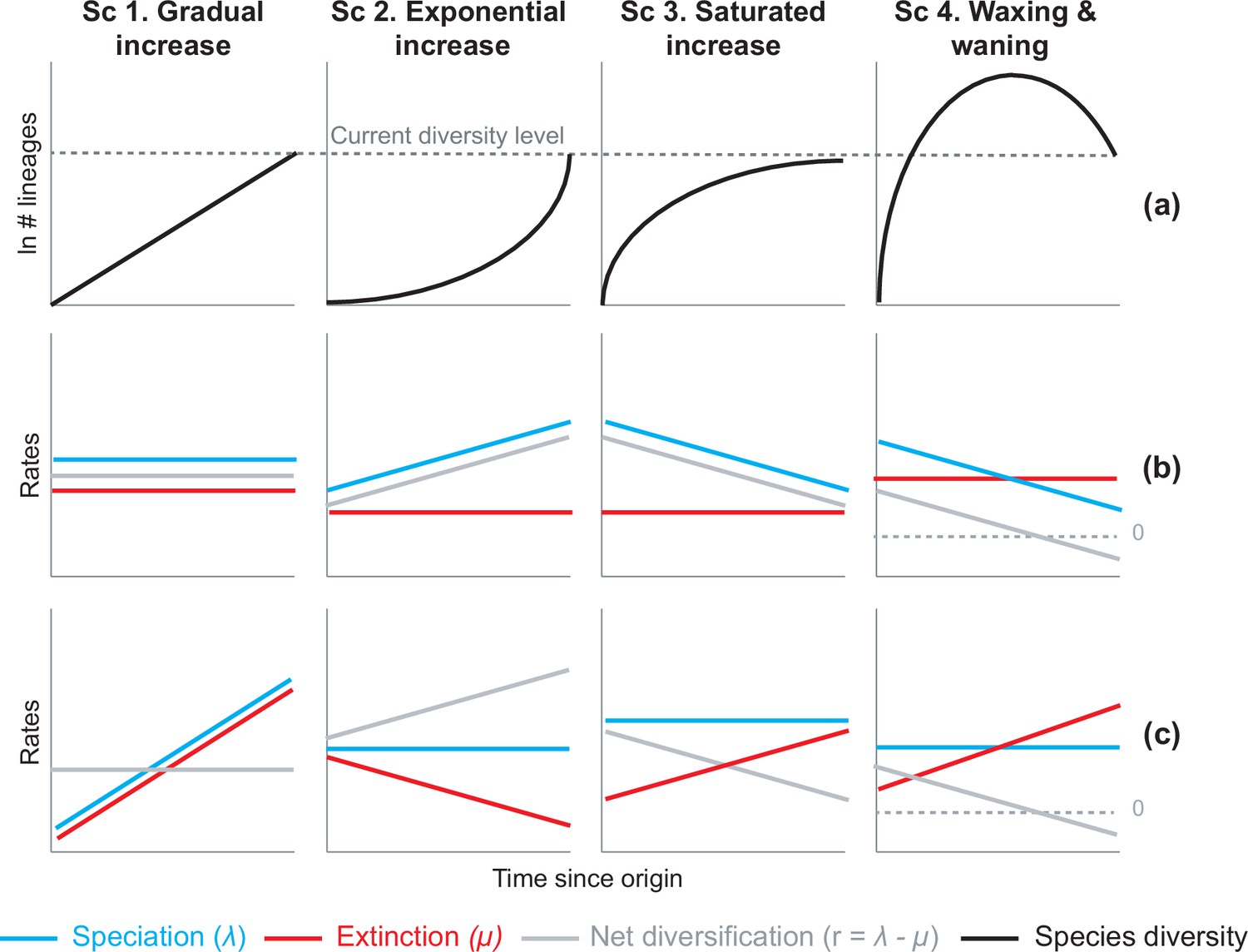
Alternative hypotheses to explain current Neotropical diversity.
(a) Main species richness dynamics through time, and (b,c) the alternative evolutionary processes that could generate the corresponding patterns. (Sc. 1a) A gradual increase of species richness could result from constant speciation and extinction rates (1b), or through a comparable increase in speciation and extinction rates (1c). (Sc. 2a) An exponential increase in species numbers could be attained through constant extinction and increasing speciation (2b), or constant speciation and decreasing extinction rates (2c). (Sc. 3a) Saturated increase scenarios, with species accumulation rates slowing down towards the present, could result from constant extinction and decreasing speciation (3b), or through constant speciation and increasing extinction rates (3c). (Sc. 4a) Waxing and waning dynamics could result from constant extinction and decreasing speciation (4b), or constant speciation and increasing extinction (4c). Waxing and waning scenarios differ from saturated increases in that extinction exceeds speciation towards the present, such that diversification goes below 0. Scenarios (b–c) represent the simplest and most general models to explain species richness patterns in (a), but other combinations of speciation and extinction rates could potentially generate these patterns; for example, an exponential increase of species (2a) could also result from increasing speciation and punctual increases in extinction, or through increasing speciation and decreasing extinction.
Figure 2 with 2 supplements
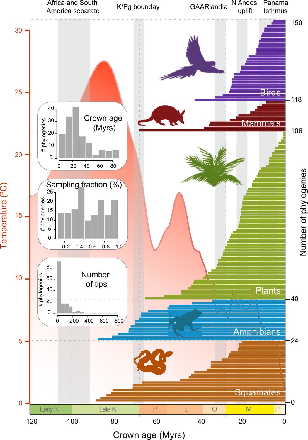
Time of origin for Neotropical tetrapods and plants.
Horizontal bars represent crown ages of 150 phylogenies analysed in this study. Shaded boxes represent the approximate duration of some geological events suggested to have fostered dispersal and diversification of Neotropical organisms. Inset histograms represent summary statistics for crown age (mean = 29.9 Myrs), sampling fraction (mean = 57%), and tree size (mean = 83.4 species/tree). Mean global temperature curve from Zachos et al., 2008. Abbreviations: K, Cretaceous; P, Paleocene; E, Eocene; O, Oligocene; M, Miocene; P, Pliocene (Pleistocene follows but is not shown); GAARlandia, Greater Antilles and Aves Ridge. Animal and plant silhouettes from PhyloPic (http://-phylopic.org/). Figure 2—source data 1 includes the dataset of plant, mammal, bird, squamate, and amphibian phylogenies and the original references for this data. Figure 2—figure supplement 1 represents summary statistics for crown age, sampling fraction, and tree size for each clade. Figure 2—figure supplement 2 includes box plots showing differences in sampling fraction, clade age, and number of species per tree for the different taxonomic groups considered in this study.
-
Figure 2—source data 1
Includes the dataset of plant, mammal, bird, squamate, and amphibian phylogenies and the original references for this data.
- https://cdn.elifesciences.org/articles/74503/elife-74503-fig2-data1-v3.docx
Figure 2—figure supplement 1
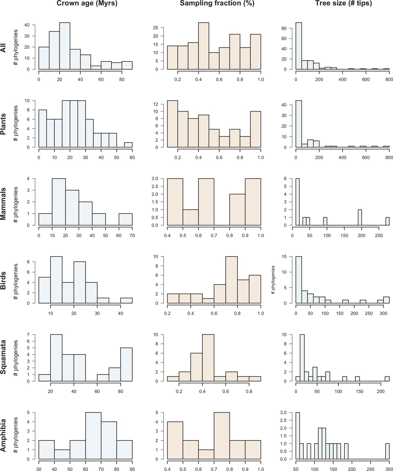
Dataset overview.
The histograms represent the clade age (crown age in million years ‘Myrs’), sampling fraction (% of described species represented in the trees) and number of tips for the 150 phylogenies of plants, mammals, birds, squamates, and amphibians.
Figure 2—figure supplement 2
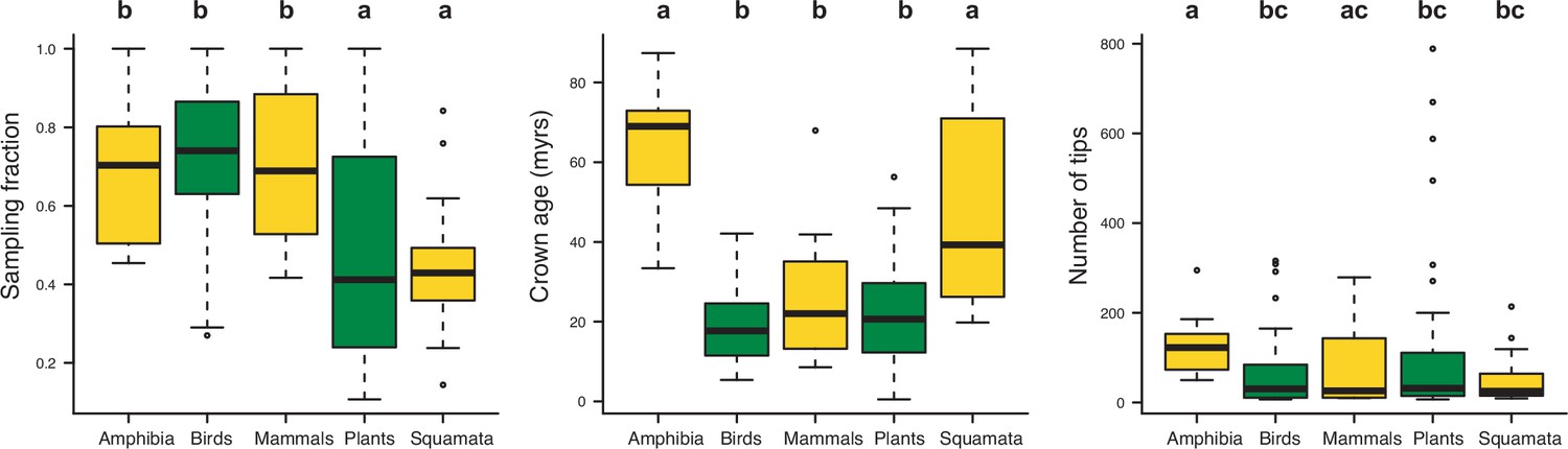
Box plots showing differences in sampling fraction, clade age (i.e., crown age), and number of species per tree (i.e., tree size) for the different taxonomic groups considered in this study (Amphibia, Birds, Mammals, Plants, Squamata).
Letters are used to denote statistically differences between groups, with groups showing significant differences in mean values denoted with different letters.
Figure 3 with 1 supplement
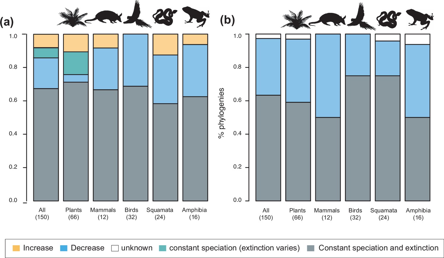
Speciation trends in 150 phylogenies of Neotropical plants and tetrapods.
The histograms show the proportion of phylogenies for which constant vs. time-variable diversification models were the best fit, as derived from (a) canonical and (b) pulled diversification rates when comparing time-dependent models against constant models. In Figure 3a, the proportion of time-variable models is subdivided by the proportion of phylogenies in which speciation rates increase through time, decrease through time, or speciation remains constant (being extinction time-variable). In Figure 3b, speciation trends are derived from present-day pulled extinction rates μp(0): negative present-day pulled extinction rates values (μp(0)<0) indicate decreasing speciation trends through time (Louca and Pennell, 2020). Positive μp(0)>0 values are possible under both increasing and decreasing speciation rates, in which case speciation trends are designed as ‘unknown’. Figure 3—source data 1 provides the data to construct a and Figure 4a. Figure 3—source data 2 provides the data to construct Figure 3b. Figure 3—figure supplement 1 shows the proportion of phylogenies fitting different pulled diversification models for a reduced dataset including only trees with more than 20 species (N=99), or with a sampling fraction over 20% (N=137).
-
Figure 3—source data 1
- https://cdn.elifesciences.org/articles/74503/elife-74503-fig3-data1-v3.docx
-
Figure 3—source data 2
Provides the data to construct Figure 3b.
- https://cdn.elifesciences.org/articles/74503/elife-74503-fig3-data2-v3.docx
Figure 3—figure supplement 1
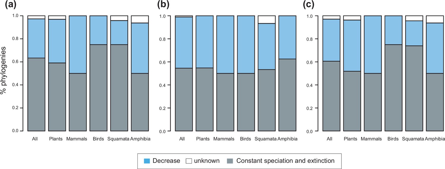
Speciation trends on 150 phylogenies of Neotropical plants and tetrapods.
The histograms show the proportion of phylogenies best fitting constant vs. time-variable diversification models, as derived from pulled diversification rates for (a) the complete dataset, (b) a reduced dataset including only trees with more than 20 species (N=99), and (c) a reduced dataset including only trees with a sampling fraction over 20% (N=137). Speciation trends are derived from present-day pulled extinction rates μp(0): negative present-day pulled extinction rates values (μp(0)<0) indicate decreasing speciation trends through time (Louca and Pennell, 2020). Positive μp(0)>0 values are possible under both increasing and decreasing speciation rates, in which case speciation trends are designed as ‘unknown’.
Figure 4 with 1 supplement
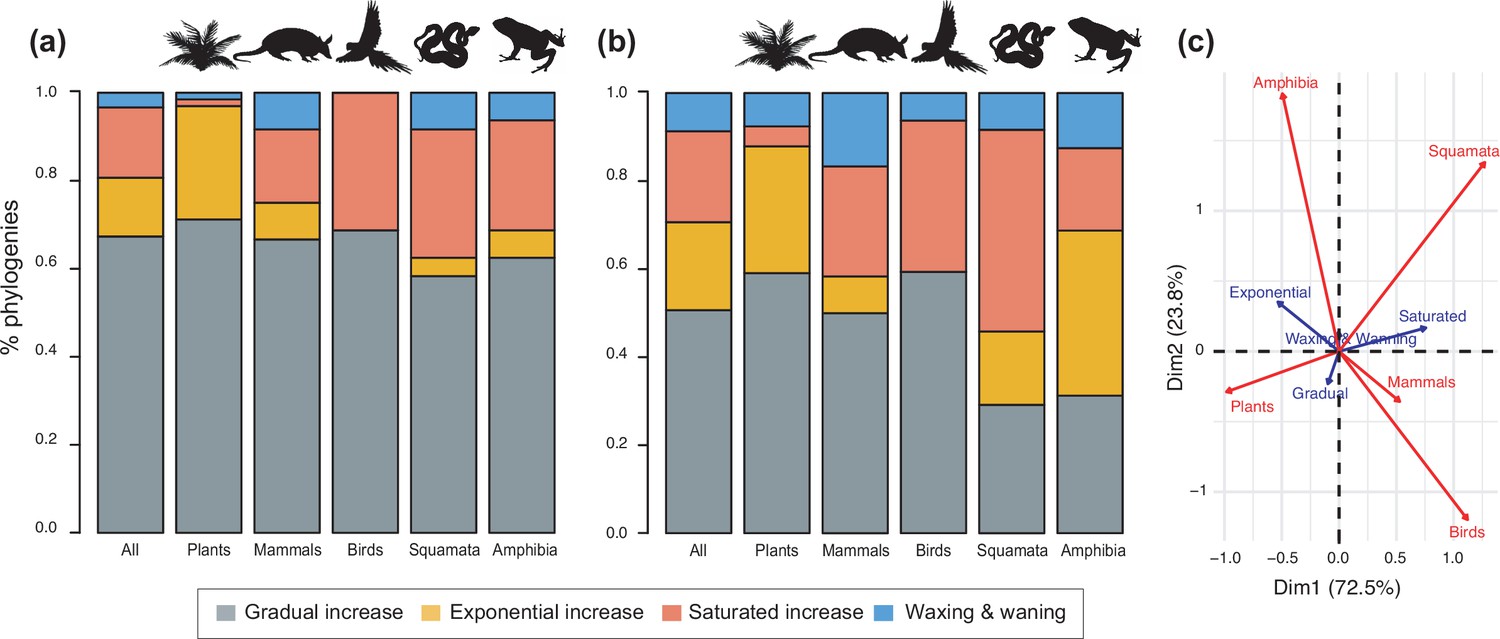
Diversity dynamics in 150 phylogenies of Neotropical plants and tetrapods.
The histograms show the proportion of phylogenies for which gradual increase (Sc. 1), exponential increase (Sc. 2), saturated increase (Sc. 3), and waxing and waning (Sc. 4) scenarios were the best fit, as derived from net diversification trends when comparing (a) time-dependent models against constant models and (b) environmental (temperature- and uplift-dependent models) against time-dependent and constant models. (c) Correspondence analysis showing the association between species richness dynamics (represented by blue arrows) and major taxonomic groups (red arrows). If the angle between two arrows is acute, then there is a strong association between the corresponding variables. Figure 4—source data 1 provides the data to construct Figure 4b and c. Source data to generate Figure 4a is provided as Figure 3—source data 1, file 2; Figure 4—figure supplement 1 shows the proportion of phylogenies best fitting different species richness dynamics for a reduced dataset including only trees with more than 20 species (N=99), or with a sampling fraction over 20% (N=137).
-
Figure 4—source data 1
Provides the data to construct Figure 4b and c.
Source data to generate Figure 4a is provided as Figure 3—source data 2.
- https://cdn.elifesciences.org/articles/74503/elife-74503-fig4-data1-v3.docx
Figure 4—figure supplement 1
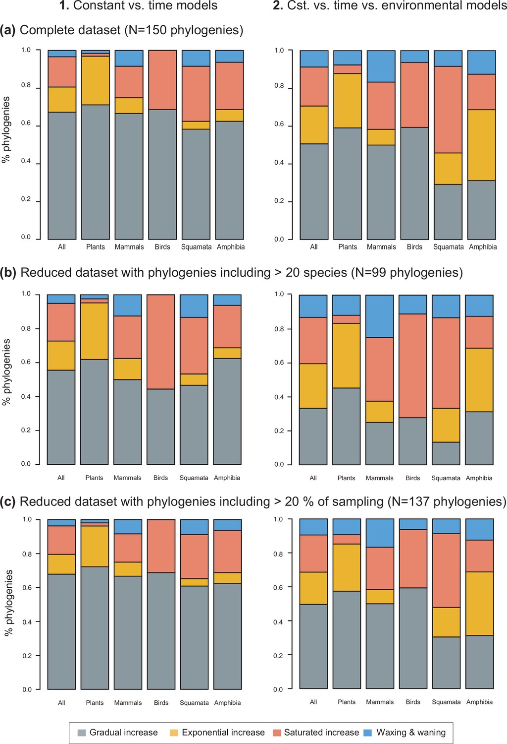
Species richness dynamics on 150 phylogenies of Neotropical plants and tetrapods.
The histograms show the proportion of phylogenies best fitting gradual increase (Sc. 1), exponential increase (Sc. 2), saturated increase (Sc. 3), and waxing and waning (Sc. 4) species richness dynamics, as derived from diversification rates when comparing (1) time-dependent against constant models, and (2) environmental (temperature- and uplift dependent) models against time-dependent and constant models. The results are reported for (a) the complete dataset, (b) a reduced dataset including only trees with more than 20 species, and (c) a reduced dataset including only trees with a sampling fraction over 20%. Abbreviation: Cst = constant.
Figure 5 with 2 supplements
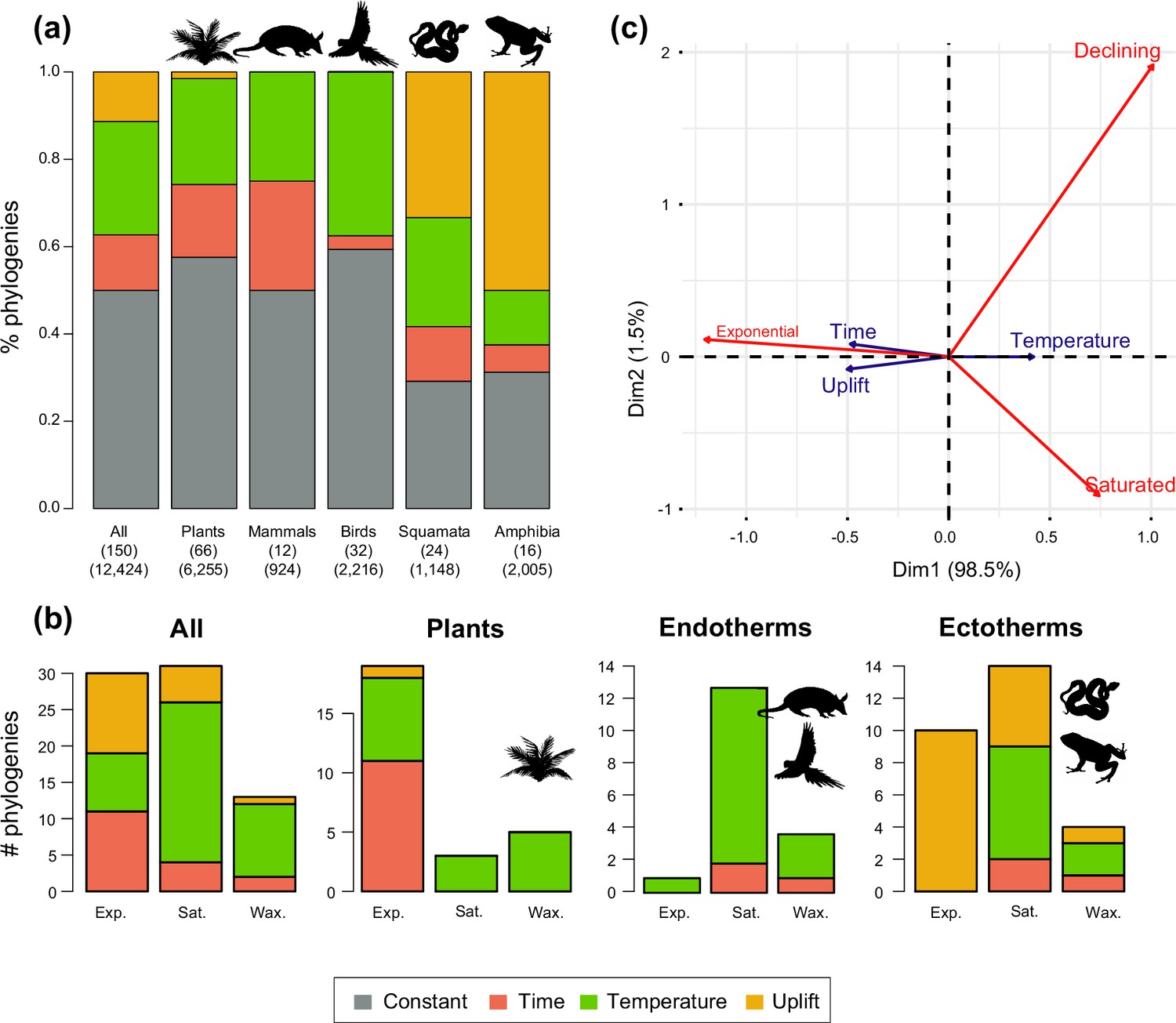
Drivers of Neotropical diversification in 150 phylogenies of Neotropical plants and tetrapods.
The histograms report the proportion of (a) phylogenies whose diversification rates are best explained by a model with constant, time-dependent, temperature-dependent, or uplift-dependent diversification. The number of phylogenies (and species) per group is shown in parentheses. (b) The histograms report the number of phylogenies whose diversification rates are best explained by a model with constant, time-, temperature-, or uplift-dependent diversification according to different species richness scenarios (Exp = Exponential increase [Sc.2], Sat = Saturated increase [Sc.3], and Wax = Waxing and waning [Sc.4]), for plants, endotherm tetrapods, ectotherms, and all clades pooled together. (c) Correspondence analysis for the pooled dataset showing the association between species richness dynamics (represented by red arrows) and the environmental drivers (blue arrows). If the angle between two arrows is acute, then there is a strong association between the corresponding variables. Figure 5—source data 1 provides the data to construct this figure. Figure 5—figure supplement 1 shows the proportion of phylogenies best fitting different paleoenvironmental models based on the most supported and second most supported model. Results are also reported for a reduced dataset including only trees with more than 20 species (N=99), or with a sampling fraction over 20% (N=137). Figure 5—figure supplement 2 shows the comparison of diversification results based on different paleotemerature curves.
-
Figure 5—source data 1
Provides the data to construct this figure.
- https://cdn.elifesciences.org/articles/74503/elife-74503-fig5-data1-v3.docx
-
Figure 5—source data 2
Shows diversification results for the most supported (lowest AIC value), and the second most supported diversification model.
- https://cdn.elifesciences.org/articles/74503/elife-74503-fig5-data2-v3.docx
Figure 5—figure supplement 1
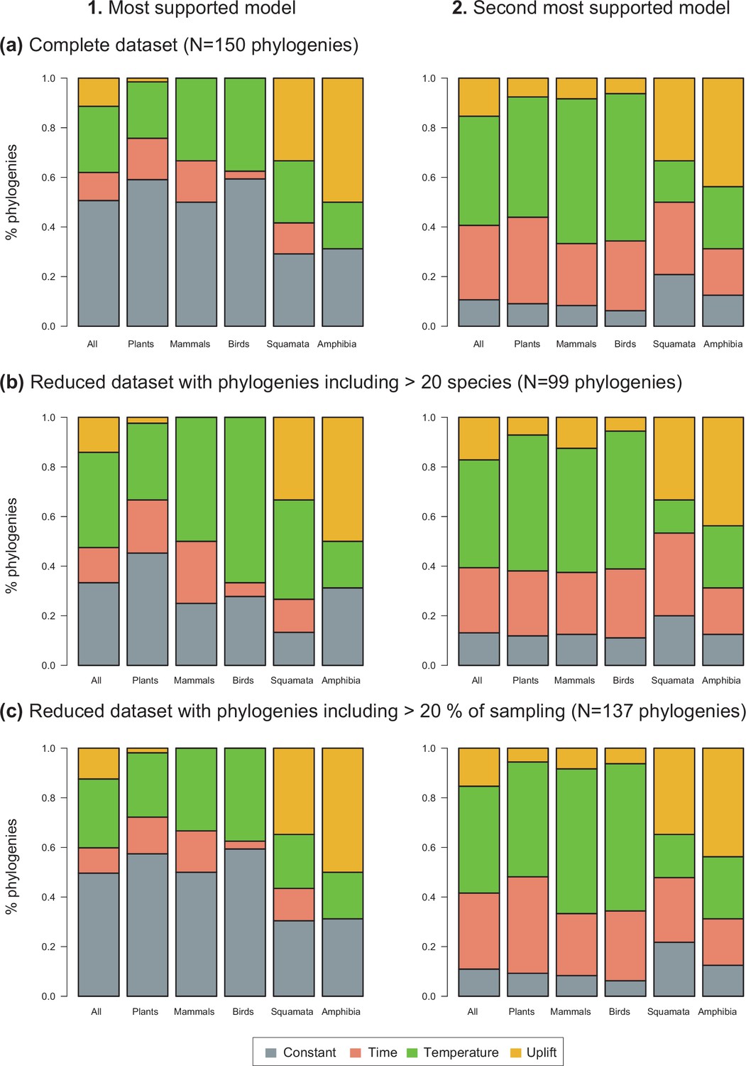
Drivers of Neotropical diversification.
The histograms report the proportion of phylogenies whose diversification rates are best explained by a model with constant, time-dependent, temperature-dependent, or uplift-dependent diversification based on (1) the most supported model (lowest AIC value), and (2) the second most supported model. The results are reported for the complete dataset (a), for a reduced dataset including only trees with more than 20 species (b), and for a reduced dataset including only trees with a sampling fraction over 20% (c).
Figure 5—figure supplement 2

Result comparisons when the temperature dependency of diversification rates is estimated based on the paleotemperature curve of Veizer and Prokoph, 2015, or Cramer et al., 2011 or Hansen et al., 2013, see Methods for details.
(a) Mean global paleotemperature estimates mostly differ in the magnitude of the changes but share the same overall trend. The histograms report (b) the proportion of phylogenies best supported by a model with diversification rates that are constant (in red), time (in blue), temperature (in green), or Andean (in orange) compared for the analyses based on different temperatures estimates.
Figure 6 with 2 supplements
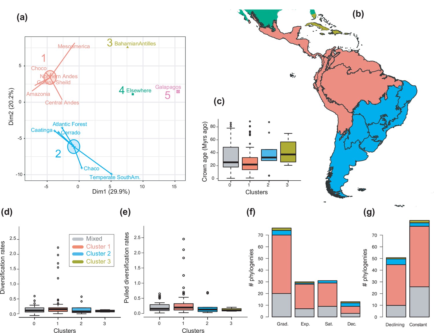
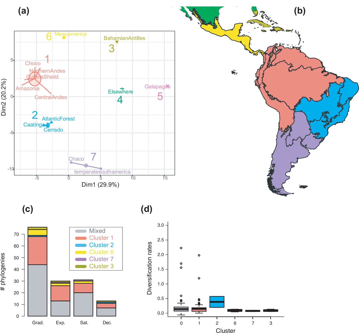
The geographical structure of long-term Neotropical diversification.
(a) Principal component analysis (PCA) representation of the five biogeographic clusters identified based on K-means clustering of 13 areas (WWF ecoregions) and 150 clades. (b) Resulting clusters (1–5) in geographic space. Colours correspond with the biogeographic clusters in (a). Thick lines delineate the original 13 ecoregions used in the analyses. (c) Box plot showing differences in crown age of the phylogenies distributed in each of the biogeographic clusters. (d) Variation in diversification and (e) pulled diversification rates (derived from the constant-rate model) across geographic clusters. (f) Number of phylogenies for which species richness scenarios Sc. 1–4 (Grad = Gradual increase [Sc.1], Exp = Exponential increase [Sc.2], Sat = Saturated increase [Sc.3], and Dec = Declining diversity [Sc.4]) were the best fit, across geographic clusters as derived from canonical diversification rates. (g) Number of phylogenies for which constant vs. declining speciation rates were the best fit, across geographic clusters as derived from pulled diversification rates. Figure 6—source data 1 provides the original data to conduct K-means clustering analyses, and generate Figure 6a; Figure 6—source data 2 provides the assignation of clades to biogeographic clusters; Figure 6—source data 3 provides the data to generate (c, d, f), and Figures 7—9; Figure 6—source data 4 provides the data to generate Figure 6; for example, Figure 6—figure supplement 1 shows the Elbow curve for K-means clustering results; Figure 6—figure supplement 2 shows biogeographic clustering and diversification results if seven clusters are considered.
-
Figure 6—source data 1
Provides the original data to conduct K-means clustering analyses, and generate Figure 6a.
- https://cdn.elifesciences.org/articles/74503/elife-74503-fig6-data1-v3.docx
-
Figure 6—source data 2
Provides the assignation of clades to biogeographic clusters.
- https://cdn.elifesciences.org/articles/74503/elife-74503-fig6-data2-v3.docx
-
Figure 6—source data 3
Provides the data to generate Figure 6c, d, f, and Figures 7—9.
- https://cdn.elifesciences.org/articles/74503/elife-74503-fig6-data3-v3.docx
-
Figure 6—source data 4
Provides the data to generate Figure 6; for example.
- https://cdn.elifesciences.org/articles/74503/elife-74503-fig6-data4-v3.docx
Figure 6—figure supplement 1
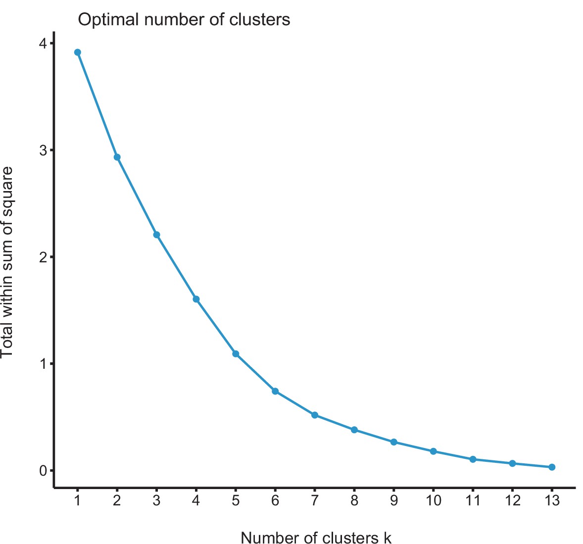
Elbow curve for K-means clustering results.
Figure 6—figure supplement 2
The geographic structure of long-term Neotropical diversification.
(a) Principal component analysis (PCA) representation of K-means clustering results for 13 areas (WWF ecoregions) and 150 clades. (b) Resulting clusters (1–5) on the geographic space. Colours correspond with the clusters of regions identified in (a), thick lines delineate the original ecoregions used in the analyses. (c) Number of phylogenies best fitting species richness scenarios Sc. 1–4 (Grad = Gradual increase [Sc.1], Exp = Exponential increase [Sc.2], Sat = Saturated increase [Sc.3], and Dec = Declining diversity [Sc.4]) across geographic clusters as derived from canonical diversification rates. (d) Variation in diversification rates (derived from the constant-rate model) across geographic clusters.
Figure 7
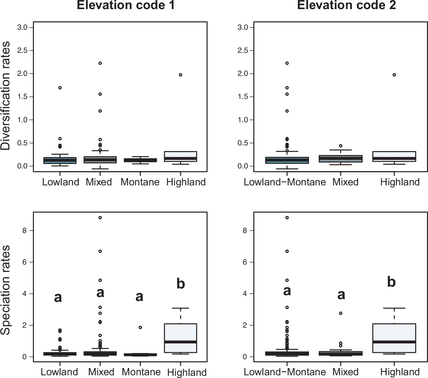
Variation in diversification rates on 150 Neotropical phylogenies of plants and tetrapods across elevation ranges.
Diversification and speciation rates are derived from the constant-rate model (Supplementary file 1A). In the elevation code 1 the montane category has been analysed separately, while in the elevation code 2 lowland and montane categories have been pooled together (see text). Letters are used to denote statistically differences between groups, with groups showing significant differences in mean values denoted with different letters. Source data to generate this figure is provided as Figure 6—source data 3.
Figure 8

Diversification rates compared across plants and tetrapods (endotherms and ectotherms).
Diversification and speciation rates are derived from the constant-rate model . Letters are used to denote statistically differences between groups, with groups showing significant differences in mean values denoted with different letters. The y-axis was cut off at 1.0 to increase the visibility of the differences between groups. Upper values for plants are therefore not shown, but the quartiles and median are not affected. Units are in events per million years. Source data to generate this figure is provided as Figure 6—source data 3.
Figure 9
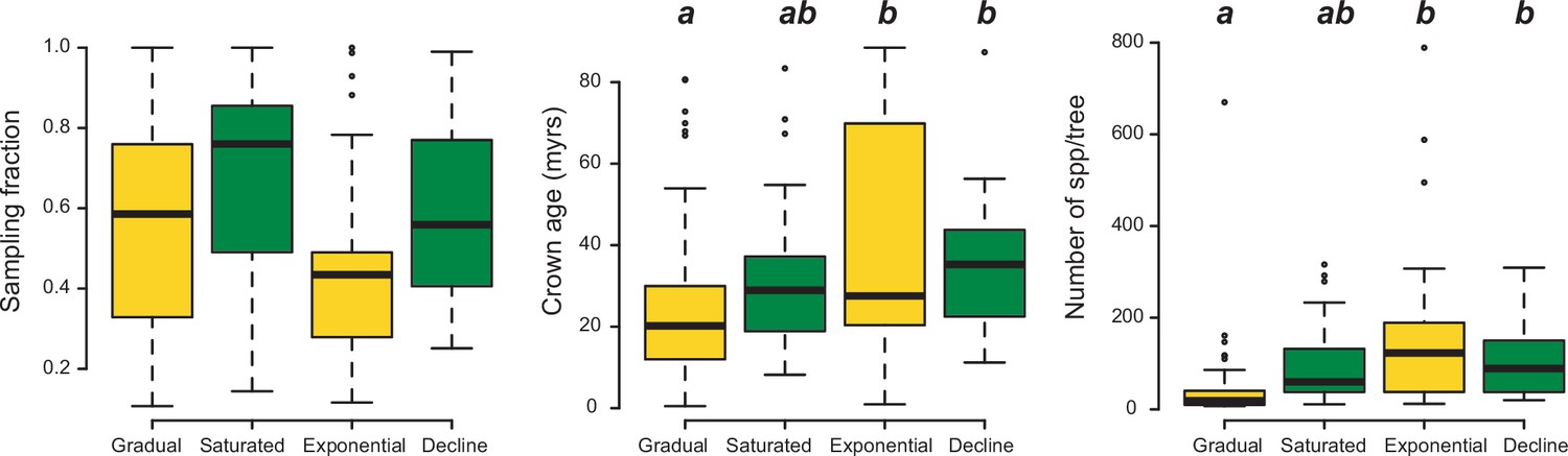
Box plots showing differences in sampling fraction, clade age (i.e., crown age), and number of species per tree (i.e., tree size) for the phylogenies supporting gradual increase (Sc. 1) vs. exponential increase (Sc. 2) vs. saturated (Sc. 3) vs. declining diversity dynamics (Sc. 4).
Sampling fraction does not differ significantly between model categories, suggesting that there is no particular bias of sampling in our study. Meanwhile, there are differences in the tree size and crown age between model categories. Letters are used to denote statistically differences between groups, with groups showing significant differences in mean values denoted with different letters. Source data to generate this figure is provided as Figure 6—source data 3.
Figure 10
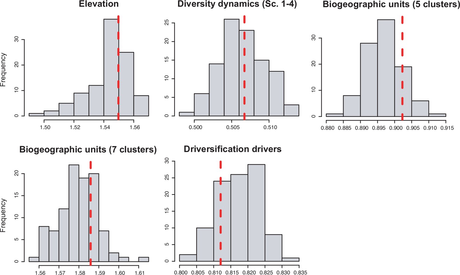
Phylogenetic signal of different multi-categorical traits.
Inferred δ-values (in red) compared to the distribution of values when the trait is randomized along the phylogeny.
Author response image 1
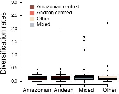
Variation in diversification rates on 150 Neotropical phylogenies of plants and tetrapods across geographic ranges.
Diversification rates are derived from the constant-rate model.
Author response image 2
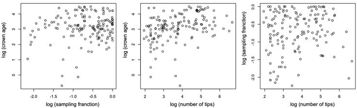
Scatterplots showing the relationship between (log transformed) sampling fraction, clade age (crown age in million years ago), and number of tips for the 150 phylogenies examined in this study.
The plots shows no association between the variables.
Author response image 3
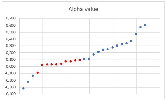
Α value of the clades which are best fit by a constant-rate model and second best fit by a temperature-dependent model.
In red those values ranging between -0.1 and 0.1. Eleven trees have constant speciation (α does not vary) and thus they are not represented here.
Tables
Table 1
Alternative species richness dynamics (Sc. 1–4) and the corresponding diversification processes (a–c) able to explain Neotropical diversity.
Species richness dynamics represent scenarios of expanding (Sc. 1–2), saturating (Sc. 3) and contracting (Sc. 4) diversity, in which speciation (λ) and/or extinction (μ) remain constant or vary through time. The number of phylogenies supporting each model is provided for all lineages pooled together, and for plants and tetrapods separately. Empirical support for each evolutionary model is based on canonical diversification rates (CDR), and pulled diversification rates (PDR), by comparing the constant model against different sets of time-variable models. For CDR, we provide as well the results (in italic) based on model comparisons including constant, time-variable, and paleoenvironmental-dependent (temperature and uplift) models.
| Diversity dynamics | CDR all (plant/tetra) | PDR all (plant/tetra) | Diversification process | Model parameters | CDR all (plant/tetra) | PDR all (plant/tetra) |
|---|---|---|---|---|---|---|
| Sc 1. Gradual increase | 101 (47/54) 76 (40/37) | 95 (39/56) | (a) Constant λ and μ | λ(t) = λ0, μ(t) = μ0 | 101 (47/54) 77 (40/37) | 95 (39/56) |
| (b) Equivalent increase in λ and μ | λ(t) = λ0eαt, μ(t) = μ0eβt, λ0 = μ0, α = β | 0 (0/0) 0 (0/0) | ||||
| (c) Both | 0 (0/0) 0 (0/0) | |||||
| Sc 2. Exponential increase | 20 (17/3) 30 (19/11) | 51 (25/26) * | (a) Increasing λ, constant μ | λ(t) = λ0eαt, α<0, μ(t) = μ0 | 9 (7/2) 9 (8/1) | 51 (25/26) * |
| (b) Constant λ, decreasing μ | λ(t) = λ0, μ(t) = μ0eβt, β>0 | 10 (10/0) 13 (11/2) | ||||
| (c) Both | 1 (0/1) 8 (0/8) | |||||
| Sc 3. Saturated increase | 24 (1/23) 31 (3/28) | (a) Decreasing λ, constant μ | λ(t) = λ0eαt, α>0, μ(t) = μ0 | 24 (1/23) 29 (3/27) | ||
| (b) Constant λ, increasing μ | λ(t) = λ0, μ(t) = μ0eβt, β<0 | 0 (0/0) 0 (0/0) | ||||
| (c) Both | 0 (0/0) 1 (0/1) | |||||
| Sc 4. Waxing and waning | 5 (1/4) 13 (5/8) | (a) Decreasing λ, constant μ | λ(t) = λ0eαt, α>0, μ(t) = μ0 | 1 (1/0) (1/5) | ||
| (b) Constant λ, increasing μ | λ(t) = λ0, μ(t) = μ0eβt, β<0 | 1 (0/0) (1/1) | ||||
| (c) Both | 3 (0/4) 8 (3/2) |
-
*
Pulled extinction rates (μp) can be useful for inferring speciation trends, for example, a negative present-day pulled extinction rate (μp(0)<0) is indicative that λ decreases through time. But the opposite is not necessarily true, that is, a positive present-day pulled extinction rate (μp(0)>0) does not necessarily indicate that λ increases through time (Louca and Pennell, 2020). Based on pulled extinction, we cannot infer either if diversification dropped below 0, and thus differentiate between the two scenarios in which λ decreases through time (3. damped increase and 4. waxing and waning dynamics). Similarly, based on pulled diversification rates, we cannot identify increases in speciation or time changes in extinction rates (scenarios 1b,c; 2a,b,c; 3b,c; 4b,c).
Table 2
Summary p value results derived from the analysis of canonical diversification (r) and pulled diversification (rp) rates.
Significant differences in the proportion of clades experiencing different diversity trajectories (based on canonical diversification rates: gradual expansions, exponential expansions, saturation or declining diversity; based on pulled diversification rates: expanding vs. declining speciation) across biogeographic units, elevations, taxonomic groups, and environmental drivers as derived from Fisher’s exact tests. Significant differences in net diversification, pulled diversification, and speciation rates across biogeographic units, elevations and taxonomic groups derive from Kruskal-Wallis chi-squared analyses. Significant results are highlighted in bold.
| Diversity trajectories | Diversification rates | Speciation rates | |||
|---|---|---|---|---|---|
| r | rp | r | rp | r | |
| Biogeographic units (5 clusters) | 0.459 | 0.252 | 0.168 | 0.083 | 0.248 |
| Biogeographic units (7 clusters) | 0.503 | 0.947 | 0.198 | 0.424 | 0.277 |
| Elevation | 0.504 | 0.839 | 0.672 | 0.277 | 0.034 |
| Elevation (lowland-montane combined) | 0.062 | 0.062 | 0.332 | 0.869 | 0.031 |
| Taxonomic groups | 0.000 | 0.126 | 0.000 | 0.000 | 0.000 |
| Environmental drivers | 0.003 | – | – | – | – |
Author response table 1
| Nb. WWF areas | Nb. species | Nb. species checked | % species checked |
|---|---|---|---|
| 1 | 7,334 | 1,918 | 26.15 |
| 2 | 2,609 | 922 | 35.34 |
| 3 | 1,339 | 529 | 39.51 |
| 4 | 687 | 370 | 53.86 |
| 5 | 307 | 215 | 70.03 |
| 6 | 218 | 184 | 84.40 |
| 7 | 127 | 103 | 81.10 |
| 8 | 111 | 91 | 81.98 |
| 9 | 77 | 67 | 87.01 |
| 10 | 46 | 35 | 76.09 |
| 11 | 32 | 30 | 93.75 |
| 12 | 11 | 11 | 100 |
| 13 | 6 | 6 | 100 |
Additional files
-
Supplementary file 1
This file contains the complete results of model selection based on (A) traditional diversification analyses comparing constant and time-dependent models; (B) traditional diversification analyses comparing constant, time-, temperature- and Andean uplift-dependent models; and (C) results for the pulled diversification rate analyses.
More details are given on each table.
- https://cdn.elifesciences.org/articles/74503/elife-74503-supp1-v3.docx
-
Supplementary file 2
This file contains all the information on the phylogenetic reconstruction and dating of Caviomorpha.
- https://cdn.elifesciences.org/articles/74503/elife-74503-supp2-v3.docx
-
Transparent reporting form
- https://cdn.elifesciences.org/articles/74503/elife-74503-transrepform1-v3.docx
Download links
A two-part list of links to download the article, or parts of the article, in various formats.
Downloads (link to download the article as PDF)
Open citations (links to open the citations from this article in various online reference manager services)
Cite this article (links to download the citations from this article in formats compatible with various reference manager tools)
Diversification dynamics in the Neotropics through time, clades, and biogeographic regions
eLife 11:e74503.
https://doi.org/10.7554/eLife.74503


