Gigapixel imaging with a novel multi-camera array microscope
- Department of Neurobiology, Duke School of Medicine, United States
- Ramona Optics Inc, United States
- Biomedical Engineering, Duke University, United States
Figures
Figure 1
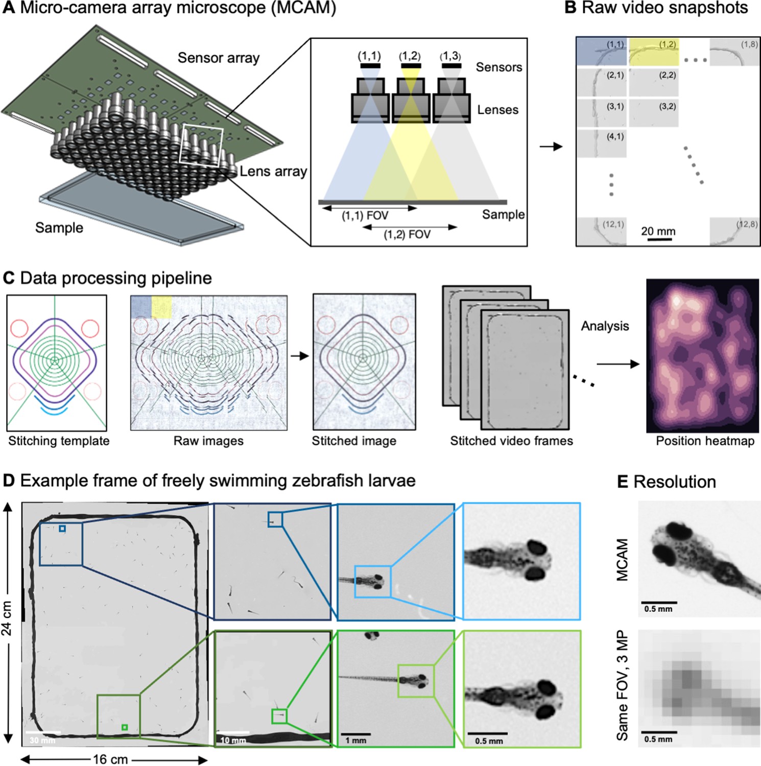
Architecture of the multiple camera array microscope.
(A) Schematic of MCAM setup to capture 0.96 gigapixels of snapshot image data with 96 micro-cameras. Inset shows MCAM working principle, where cameras are arranged in a tight configuration with some overlap (10% along one dimension and 55% along the other) so that each camera images a unique part of the sample and overlapping areas can be used for seamless stitching (across 5 unique test targets and all included model organism experiments) and more advanced functionality. (B) Example set of 96 raw MCAM frames (8x12 array) containing image data with an approximate 18 µm two-point resolution across a 16x24 cm field-of-view. (C) Snapshot frame sets are acquired over time and are combined together via a calibration stitching template to reconstruct final images and video for subsequent analysis. An example of an analysis is a probability heatmap of finding a fish within the arena at a given location across an example imaging session. (D) Example of one stitched gigapixel video frame of 93 wildtype zebrafish, 8 days post fertilization, selected at random from an hour-long gigapixel video recording. (E) Resolution comparison of an example larval zebrafish captured by the MCAM and from a single-lens system covering a similar 16x24 cm FOV using a 3 MP image sensor (but capable of high-speed video capture).
Figure 2
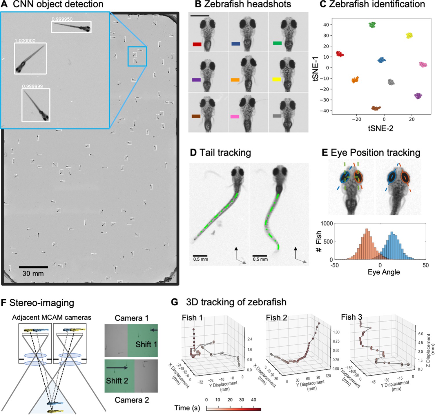
Gigapixel high-resolution imaging of collective zebrafish behavior.
(A) Example frame of stitched gigapixel video of 130 wildtype zebrafish, 8 days old (similar imaging experiment repeated 11 times). An object detection pipeline (Faster-RCNN) is used to detect and draw bounding boxes around each organism. Bounding boxes include detection confidence score (for more details see Methods). Each bounding box’ image coordinates is saved and displayed on stitched full frame image. Zoom in shows three individual fish (blue box). Scale bar: 1 cm. (B) Headshots of nine zebrafish whose images used to train a siamese neural network (see Methods, Appendix 1—figure 6). Colors indicate the fish identity used to visualize performance in (C). Each fish has a distinct melanophore pattern, which are visible due to the high resolution of MCAM. Scale bar: 1 mm. (C) Two-dimensional t-SNE visualization of the 64-dimensional image embeddings output from the siamese neural network, showing that the network can differentiate individual zebrafish. For 9 zebrafish, 9 clusters are apparent, with each cluster exclusively comprising images of one of the 9 fish (each dot is color-coded based on ground truth fish identity), suggesting the network is capable of consistently distinguishing larval zebrafish (62 training epochs, 250 augmented images per fish). (D) Close-up of three zebrafish with tail tracking; original head orientation shown in gray (bottom right). (E) Automated eye tracking from cropped zebrafish (see Methods for details); results histogram of eye angles measured on 93 zebrafish across 20 frames. (F) Optical schematic of stereoscopic depth tracking. The depth tracking algorithm first uses features to match an object between cameras (top) and then calculates the binocular disparity between the two cameras to estimate axial position with an approximate resolution of 100 µm along z (verified in calibration experiments at 50 axial positions). (G) Example 3D trajectories for 3 zebrafish from recorded gigapixel video of 93 individuals, with z displacement estimated by stereoscopic depth tracking.
Figure 3
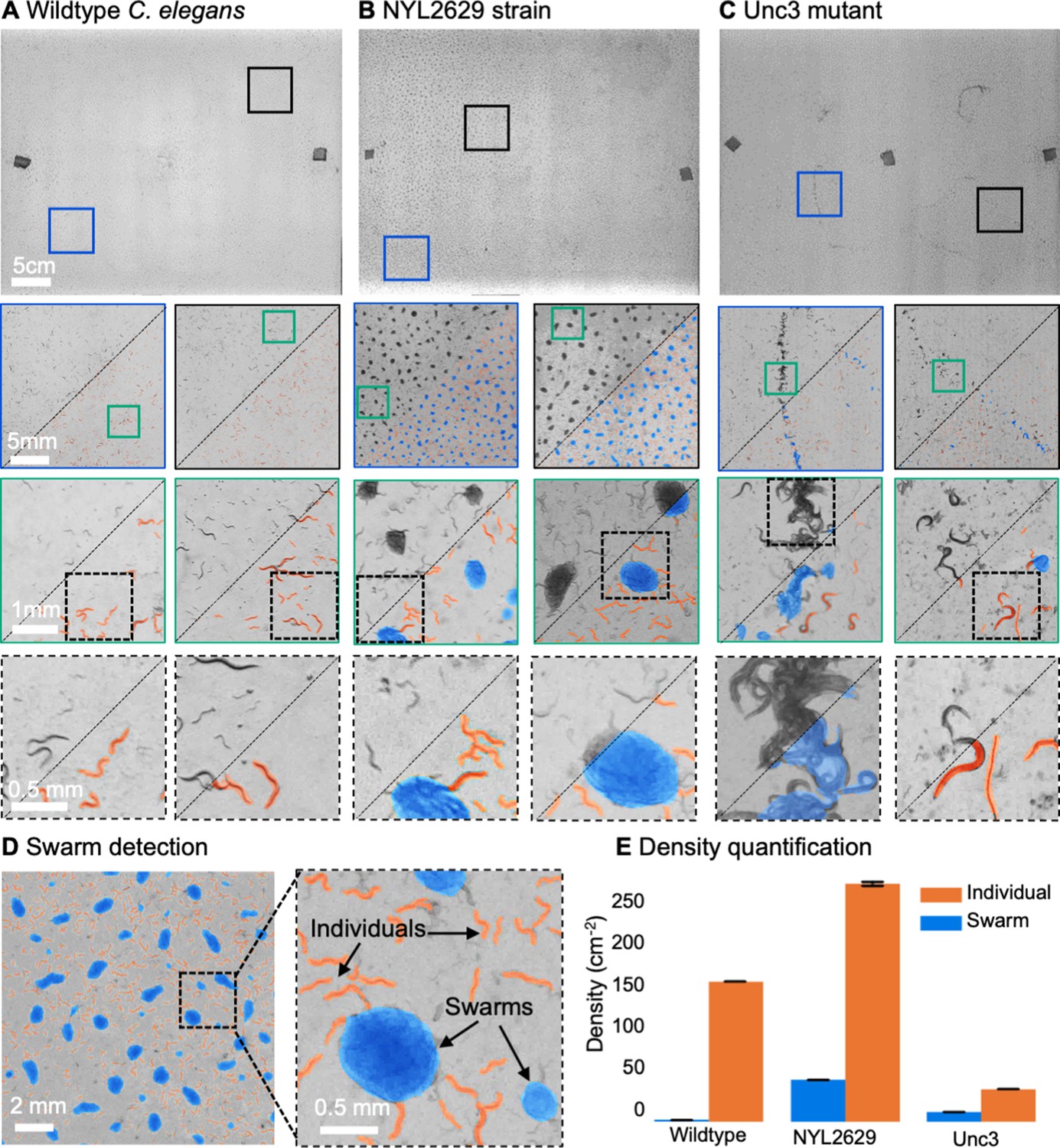
MCAM imaging of swarming behavior in C. elegans.
(A) Wild type C. elegans (N2 line) spread across the entire arena uniformly. Consecutive zoom ins show no significant swarming behavior. Approx. 30,000 organisms resolved per frame (similar imaging experiment repeated 4 times). (B) NYL2629 C elegans strain shows a periodic tiling of the petri dish over the majority of the arena as C. elegans form swarm aggregates that can be automatically detected. Approximately, 58,000 organisms resolved per frame. (C) Unc3 mutant C. elegans exhibit large wavefront swarms of activity, without the periodic tiling seen in the NYL2629 strain. Unc3 genotype inhibits a significant swarming behavior and causes swarms, annotated in blue, all over the entire arena. Our system provides sufficient resolution across a large field-of-view to enable studying behavioral patterns of C. elegans. In all cases the imaging was performed after day 3 of starting the culture. Videos 4–6 allow viewing of full video. Entire gigapixel video frames viewable online, ~8000 organisms resolved per frame. (D) Segmentation of swarms (blue) and individual C. elegans (orange) using a U-shaped convolutional network allows the automatic creation of binary identification masks of both individual worms and swarms. After segmentation, we used a pixel-connectivity-based method to count the number of objects (worms or swarms) in each gigapixel segmentation mask. (E) Bar graph quantifying density of worms within and outside of swarms for the different strains in A-C. Error bars indicate S.E.M across the arena. Mean worm density (number of worms/cm2) for wildtype 154+–0.254, NYL2629 262 +- 1.126, Unc3 36+–0.203. Mean swarm density (swarms/cm2) for wildtype 1.85+–0.01, NYL2629 45.92 +- 0.073, Unc3 10.65+–0.025. While more wild type worms than Unc3 are plated, wild type worms form far fewer swarms (p=2.3 x 10–66, Cohen’s d=0.96) 1 sided t-test. For more details, see Methods.
Figure 4
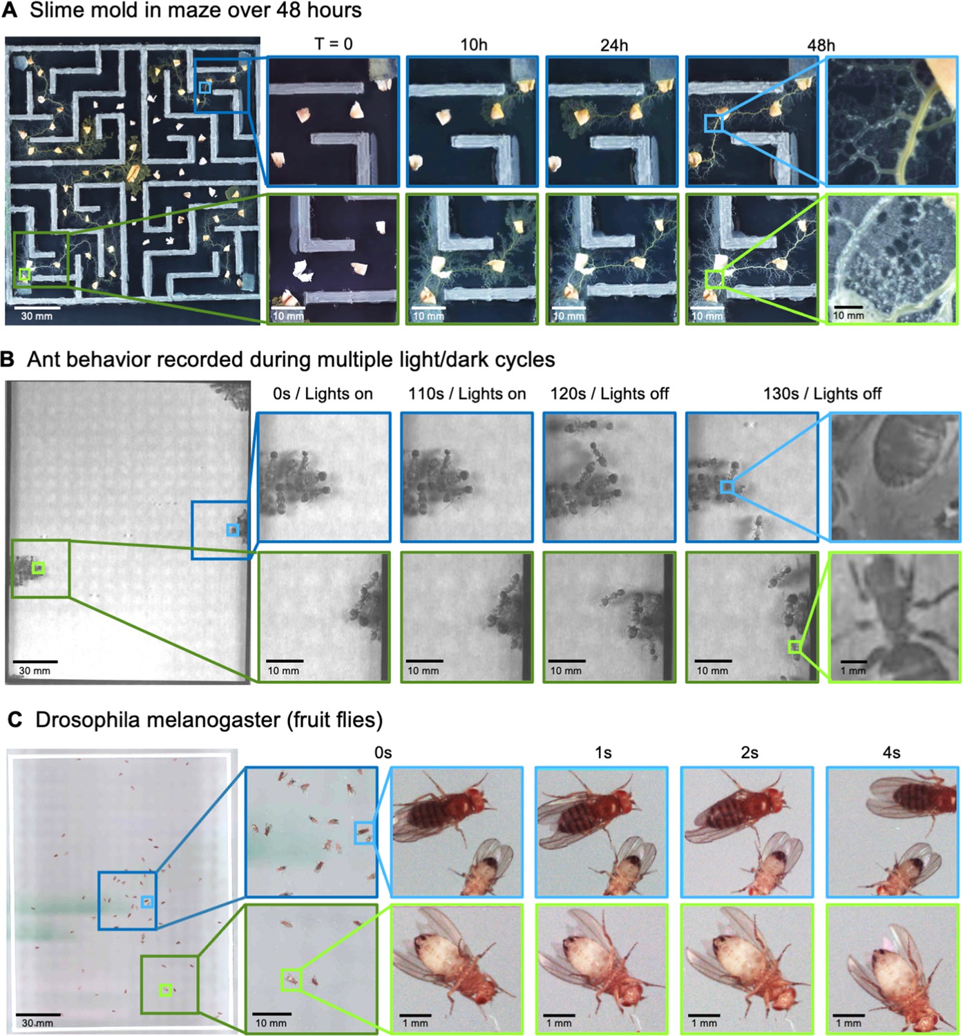
MCAM imaging of behaviors in multiple small organisms.
(A) Gigapixel video of slime mold (P. polycephalum) growth on maze (16.5 cm per side). Four mold samples were taken from a seed inoculation on another petri dish and placed in four corners of the maze. Recording for 96 hr shows the slime mold growth within the maze (Video 7). highlighting the MCAM’s ability to simultaneously observe the macroscopic maze structure while maintaining spatial and temporal resolution sufficient to observe microscopic cytoplasmic flow (imaging experiments with P. polycephalum repeated 5 times). (B) Gigapixel video of a small colony of Carpenter ants during light and dark alternations. Overall activity (velocity) of ants measured with optical flow increased during light off versus light on phases. Full MCAM frame observes Carpenter ant colony movement and clustering within large arena, while zoom-in demonstrates spatial resolution sufficient for leg movement and resolving hair on abdomen (imaging experiments with Carpenter ants repeated 2 times). See Video 10. (C) Adult Drosophila gigapixel video frame showing collective behavior of several dozen organisms at high spatial resolution, with insets revealing fine detail (e.g. wings, legs, eyes) during interaction (imaging experiments with adult Drosophila repeated 2 times). See Video 11.
Appendix 1—figure 1
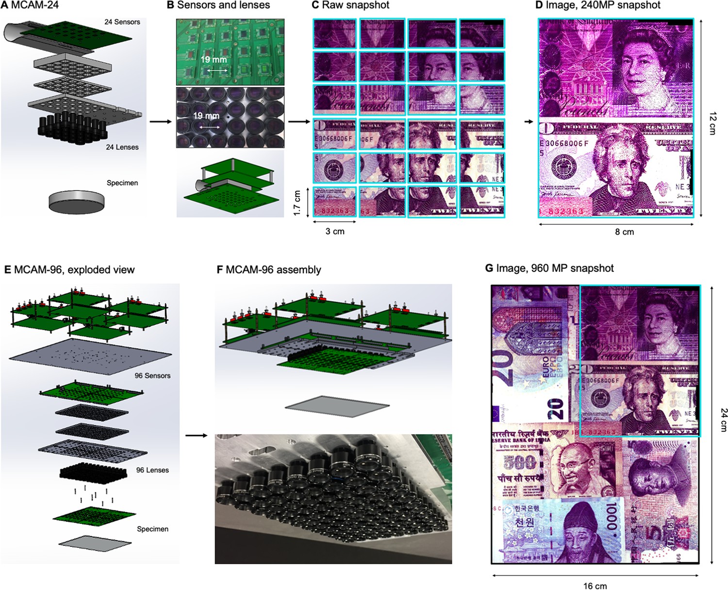
MCAM hardware.
(A) MCAM-24 hardware arrangement in an exploded view, showing an array of 24 individual CMOS sensors (10 MP each) integrated onto a single circuit board with 24 lenses mounted in front. (B) Photos of bare MCAM-24 CMOS sensor array and lens array. (C) Example snapshot of 24 images acquired by MCAM-24 of common currency. (D) Stitched composite. (E) Four MCAM-24 units are combined to create the gigapixel MCAM-96 setup, with 96 sensors and lenses tiled into a uniformly spaced array for a total of 960 MP captured per image snapshot. (F) CAD render and photo of complete MCAM-96 system. (G) Example stitched composite from MCAM-96, with MCAM-24 field-of-view shown in teal box.
Appendix 1—figure 2
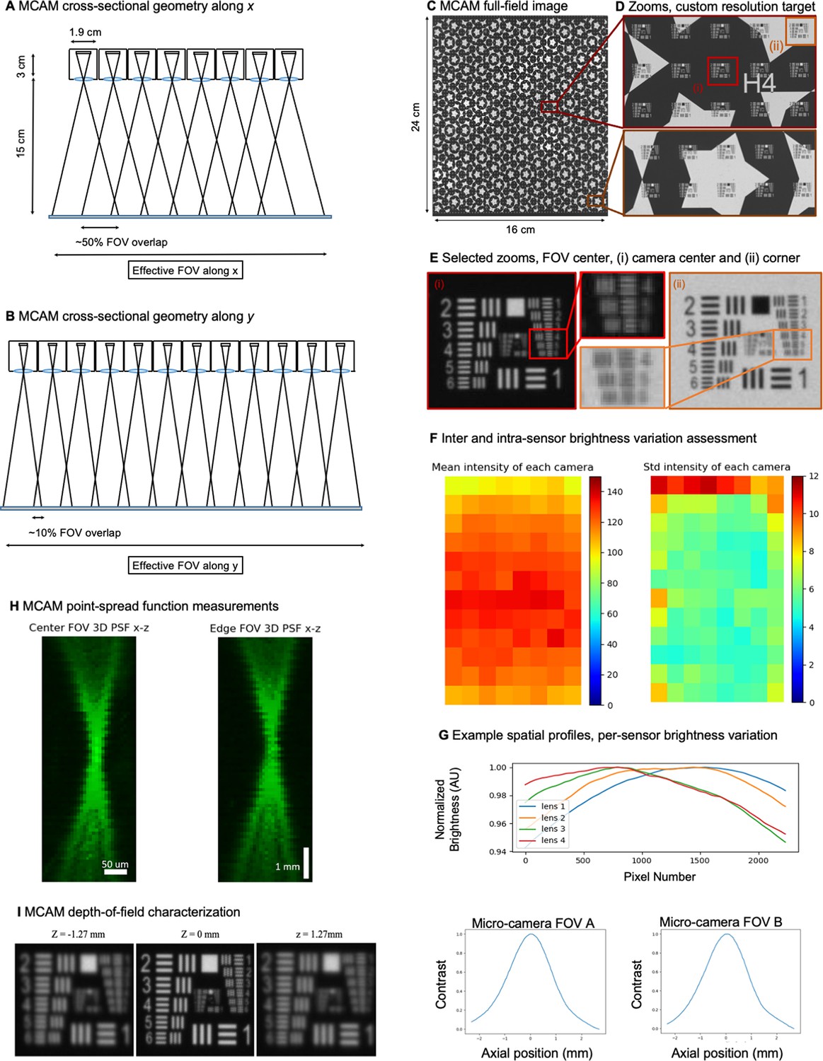
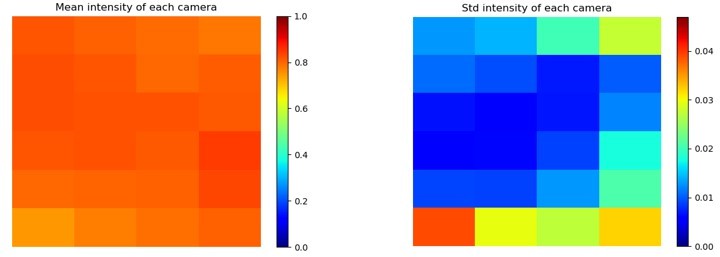
96-camera MCAM geometry, resolution, and brightness measurements.
(A) MCAM geometry cross-section along x direction of 8x12 array. The rectangular image sensor exhibits a longer dimension along x, yielding camera images sharing >50% FOV overlap for depth tracking and dual-fluorescence imaging. (B) MCAM geometry cross-section along y direction of 8x12 array, where image sensor’s shorter dimension leads to approximately 10% overlap between adjacent camera FOVs to facilitate seamless image stitching. (C) Full field-of-view MCAM-96 image of a custom-designed resolution target covering over 16 cm x 24 cm, with (D) Zoom-ins. (E) Two further zoom-ins from marked boxes in (d) that lie at the center and edge of a single camera FOV. Resolution performance varies minimally across each camera FOV. For this custom-designed resolution target, Element 4 at the resolution limit exhibits a 22.10 µm full-pitch line pair spacing, Element 5 a 19.68 µm full-pitch line pair spacing, Element 6 a 17.54 µm full-pitch line pair spacing. The MCAM consistently resolves Element 5 but at times does not fully resolve Element 6, leading to our approximation of 18 µm resolution. (F) Plots of inter- and intra-camera brightness variation for a uniformly diffuse specimen. (left) Mean of raw pixel values for each camera within the 8x12 array, and standard deviation across all per-sensor raw pixel values for each sensor within the 8x12 array. (G) Plot of average normalized pixel value across the vertical camera dimension for 4 randomly selected micro-cameras when imaging a fully diffuse target. Relative brightness varies <6% across the array. Primary contributions arise from illumination, lens, and sensor-induced vignetting effects. As described in Appendix 1 – Image stitching below, digital flat-field correction is used for correction. (H) X-Z and Y-Z cross-sections of point-spread function (PSF) measurements acquired by a single micro-camera at FOV center and edge. For acquisition, monolayer of 6 µm fluorescent microspheres was mechanically translated in 100 µm steps axially across 7 mm. (I) Depth of field (DOF) characterization data. (left) USAF target images at axial locations used to identify axial range across which resolution stays within a factor of 2 of its maximum value as DRes = 2.54 mm. (right). Plots of normalized mean USAF target image gradient magnitude as a function of axial position across 5 mm depth range with average FWHM DCon = 1.95 mm.
Appendix 1—figure 3
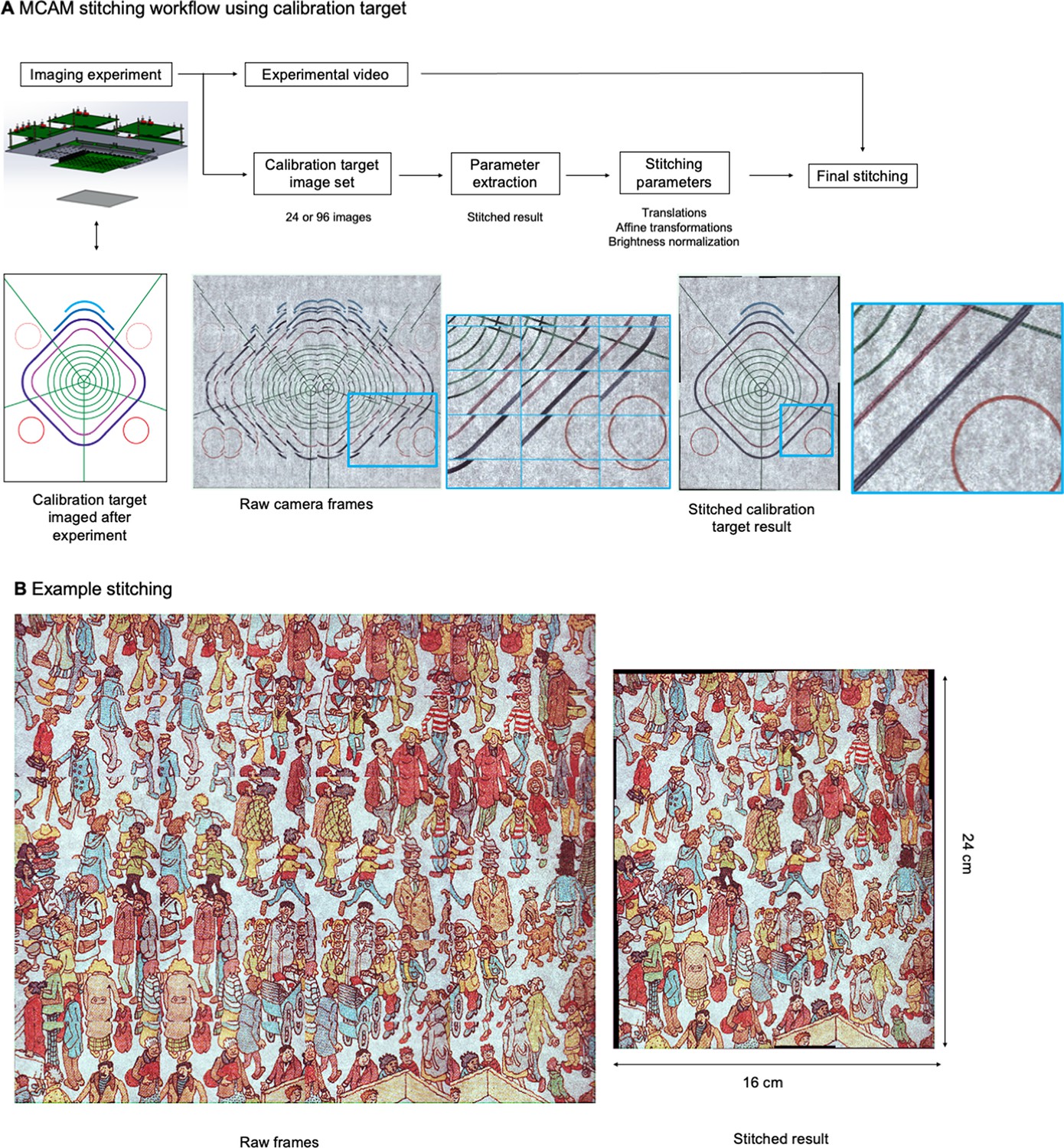
MCAM Stitching Process.
(A) Schematic of workflow of the MCAM stitching process. (B) Example raw frame are stitched together using parameters extracted from calibration target.
Appendix 1—figure 4
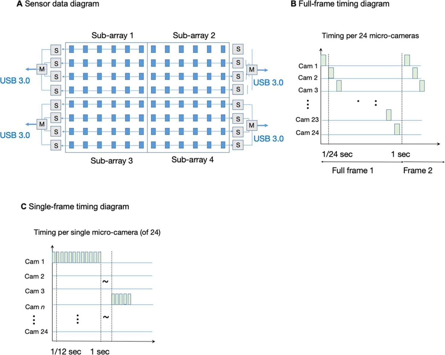
MCAM data management and timing.
(A) MCAM-96 (0.96 gigapixel) data layout and readout geometry from four MCAM-24 sub-arrays. (B) Timing sequence of frame data for each MCAM-24 running in full-frame mode. (C) Timing sequence of frame data for each MCAM-24 running in single-frame mode.
Appendix 1—figure 5
Object detection using gigapixel video.
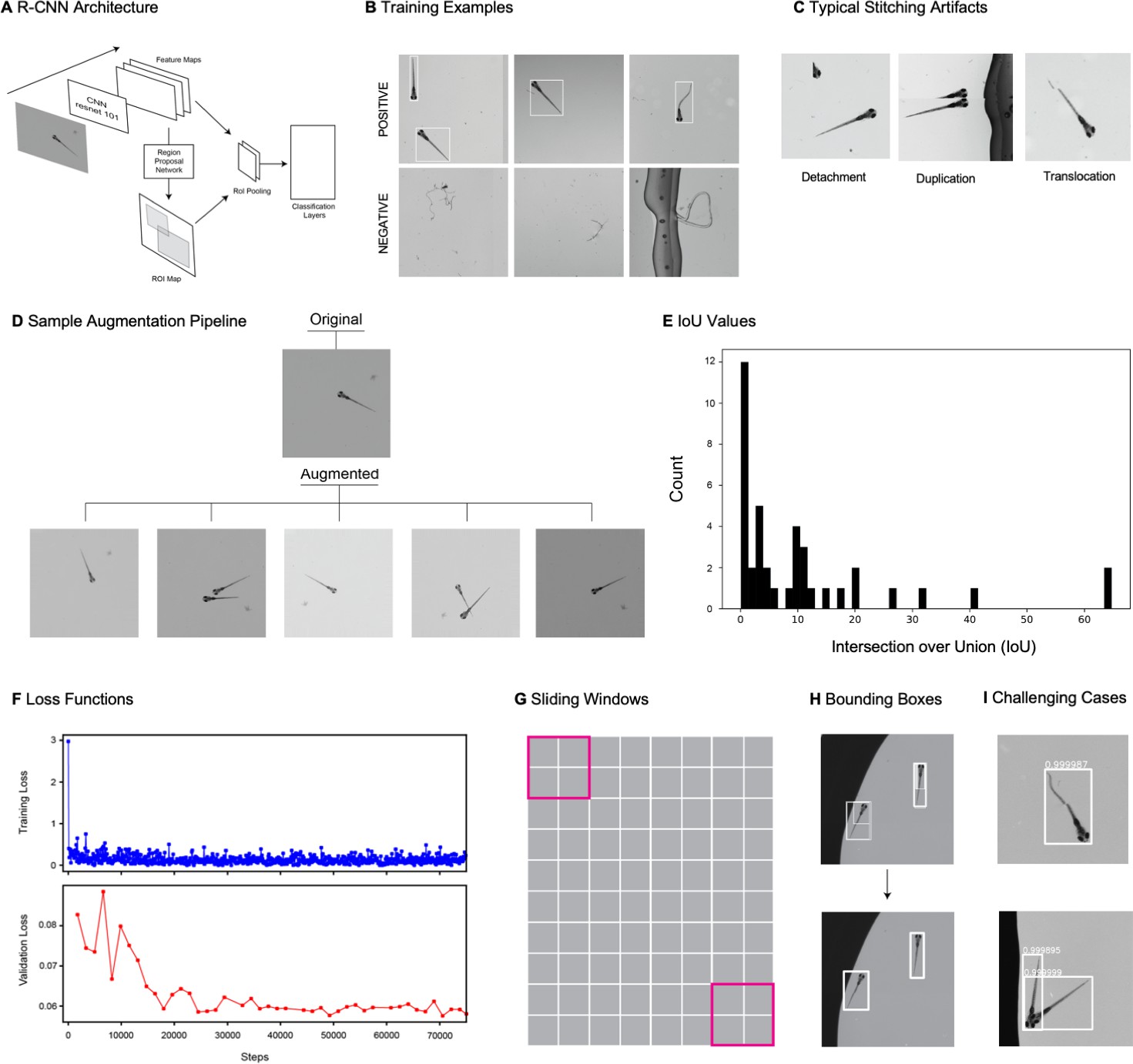
(A) Faster R-CNN architecture. The architecture consists of a traditional CNN (in this case a resnet-101 backbone) for feature extraction, which feeds into a region proposal network (RPN) and an RoI pooling layer. The RPN generates an ROI map, proposing potential locations of objects. The features and potential object locations are fed to an RoI pooling layer which normalizes the size of each bounding box before the information is fed into a classifier that predicts the object type for each ROI. (B) Examples of positive (top row) and negative (bottom row) examples used for training the faster R_CNN. (C) Examples of the main types of stitching artifacts, including detachment (left), duplication (middle), and translocation (right). See main text in Appendix 1: Large-scale object detection pipeline for more details. (D) Augmentation pipeline example: top image is the original image, and the bottom five images are five augmented instances generated from the original. We generated five augmented instances of each training image in our training data. (E) Histogram of intersection over union values for all fish from our actual data (test data and unaugmented training data). (F) Loss function in training and validation data during 75000 step training of the faster-R-CNN. (G) Depiction of sliding windows used for inference over stitched images. (H) Example from a fraction of a stitched frame showing multiple fish of the original set of multiple overlapping bounding boxes, and the final set of unique bounding boxes enveloping individual fish (obtained using a combination of a nonmax suppression followed by a proper subset filter, as described in Appendix 1). (I) Examples of successfully detected zebrafish in the presence of stitching artifacts (top) and occlusion (bottom). Please see additional example in Appendix 1—Video 3.
Appendix 1—figure 6
Siamese network with triplet loss differentiates individual zebrafish.
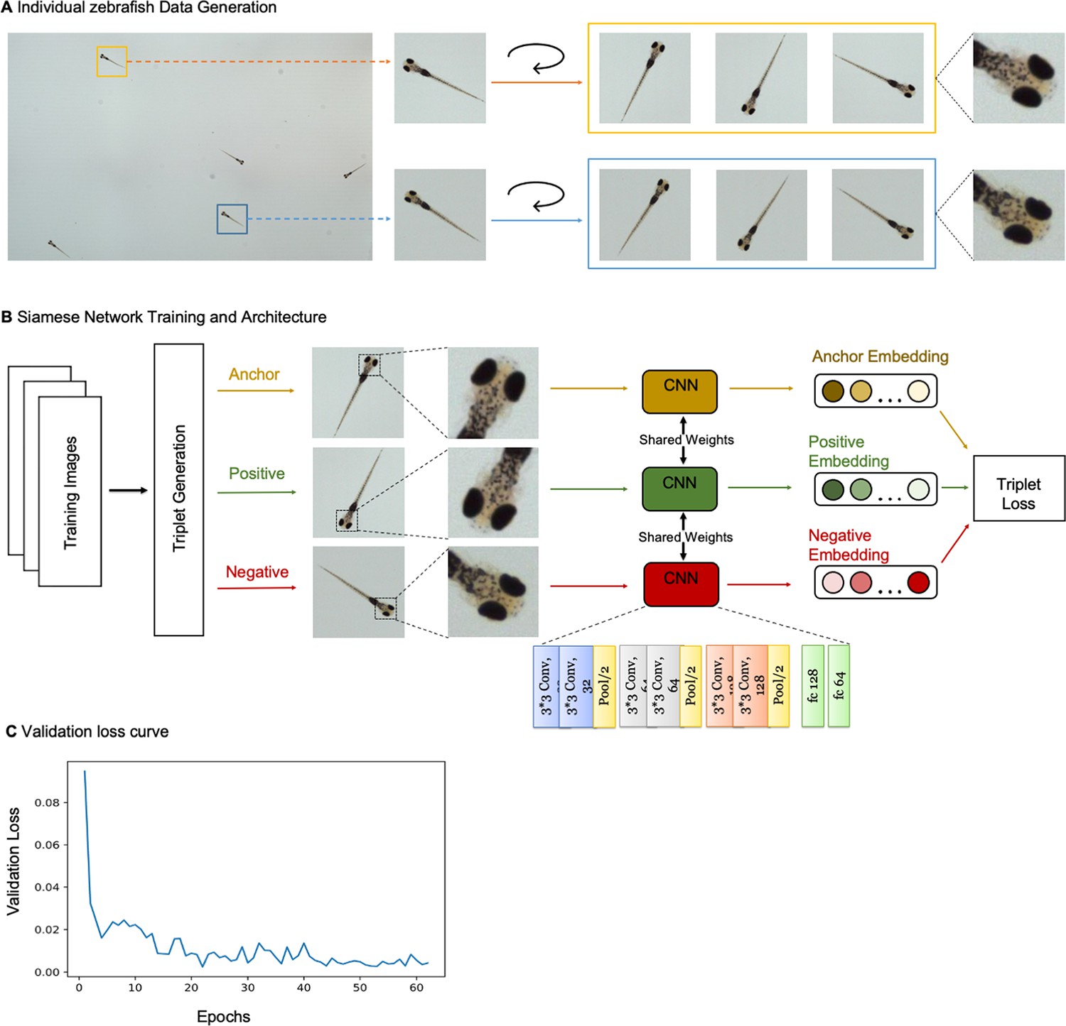
(A) Strategy for training data generation from two example larval zebrafish in a section of the behavioral arena. Bounding boxes from Faster-RCNN algorithm were used to crop fish from images captured by MCAM. Data was augmented via rotations of cropped images by a random angle (θ≤360°). Individual differences, such as melanophore patterns are discernable in training images and presumably used to distinguish larval zebrafish. (B) Cartoon of Siamese Network with triplet loss architecture used to differentiate larval zebrafish. Three subnetworks with shared weights and parameters have six convolutional layers and two fully connected layers. The subnetworks receive triplets containing two training images of the same fish (anchor and positive) and a third training image of a different fish (negative) and generate 64-dimensional embeddings. Triplet loss compares the anchor to the positive and negative inputs, and during training maximizes the Euclidean distance between the anchor and negative inputs and minimizes the distance between the anchor and positive inputs. (C) Validation loss versus epoch for training shown in Figure 2C. Loss decreases and ultimately converges over training. Here, the network is trained for 62 epochs, which takes approximately 20 minutes.
Appendix 1—figure 7
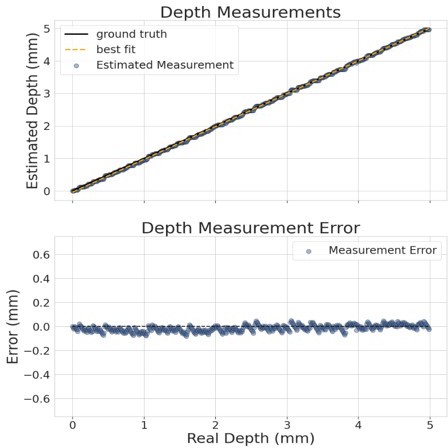
MCAM Stereoscopic imaging.
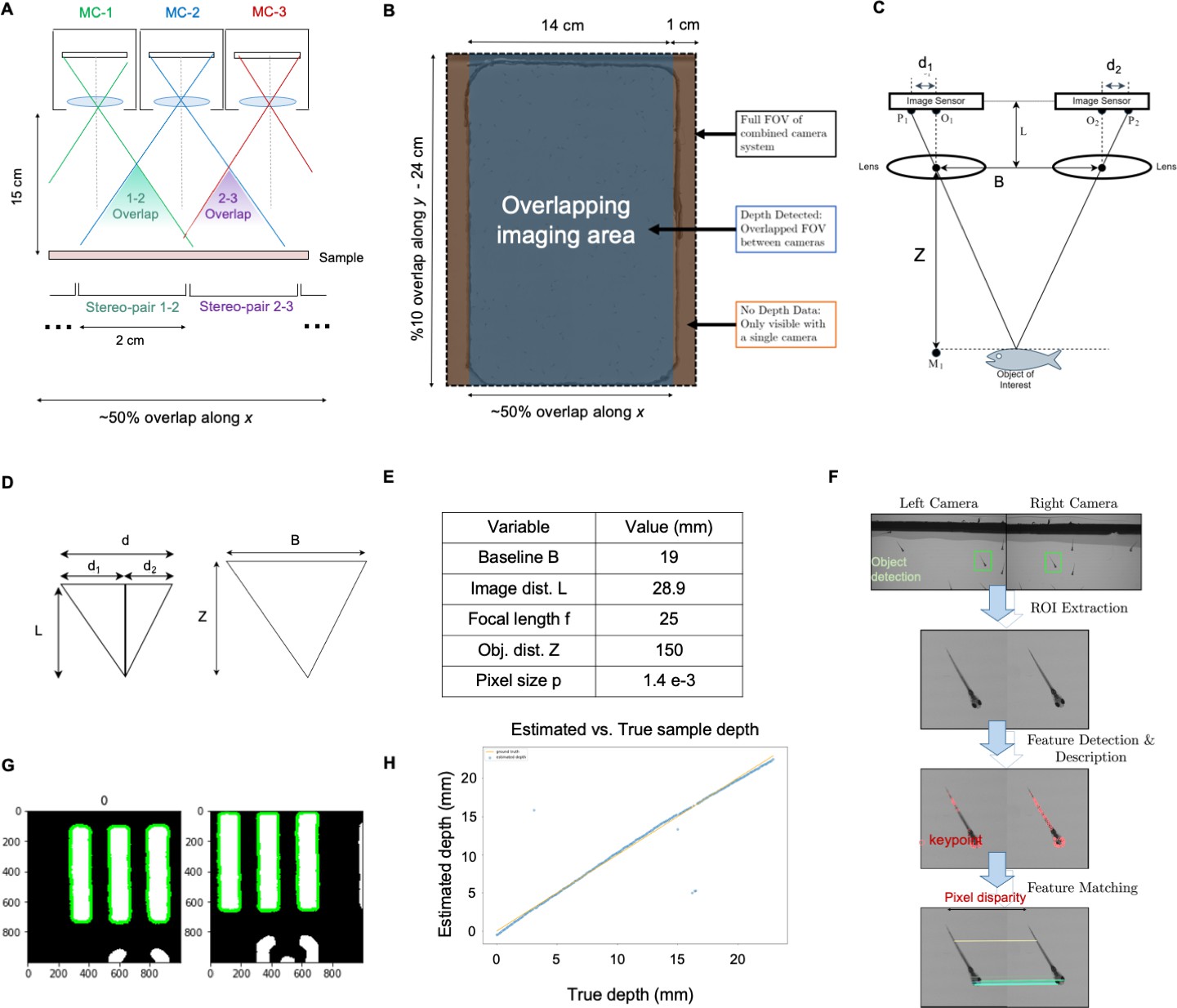
(A) Diagram of MCAM imaging geometry for stereoscopic depth tracking with marked stereo-pair regions (B) Stereo-pair regions exist within an overlapping imaging area (other than a small boarder region). (C) Schematic of stereoscopic imaging arrangement with variables of interest marked. Object distance (Z) is calculated via trigonometry, after digital estimation of d1 and d2. (D) (d) Similar triangles from (c) used for depth estimation via Equation 1. (E) Table of variables and typical experimental values. (F) Feature Detection and Matching Pipeline. Matching ROI extracted from a stereo pair, a feature description algorithm is applied to each image and are then matched to compute d1 and d2 for pixel disparity measurement (G, H) Experimental results, indicating approximately 100 µm resolution over the entire depth range. Outlying points are due to the inability to accurately match image pair features. For more see main text of Appendix 1: Depth tracking section.
Appendix 1—figure 8
Single and dual channel wide field fluorescence imaging with the MCAM.
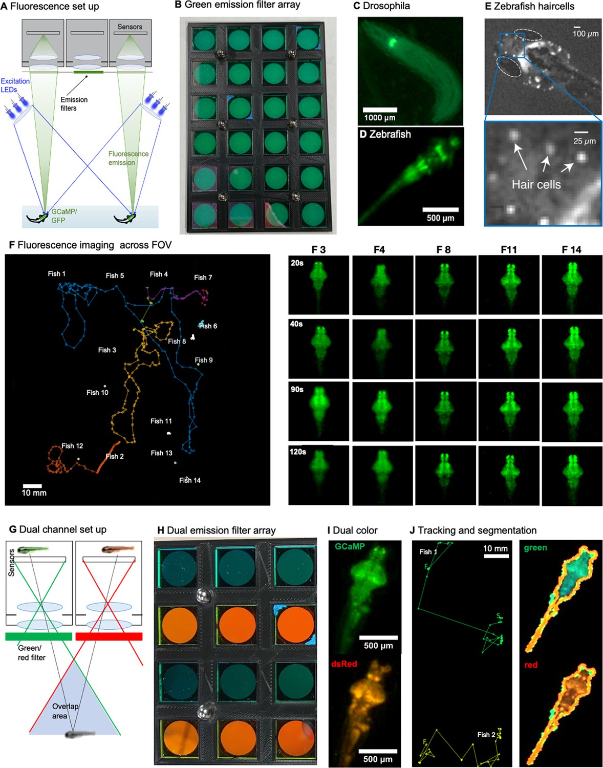
(A) Schematic of MCAM fluorescence imaging set up. Wide-field single-channel fluorescence imaging was implemented with two external high-power LEDs with a wavelength of 470 nm (Chanzon, 100 W Blue) for excitation. Each excitation source additionally included a short-pass filter (Thorlabs, FES500). We then inserted a custom-designed emission filter array containing 24 filters (525±25.0 nm, Chroma, ET525/50 m) directly over the MCAM imaging optics array to selectively record excited green fluorescent protein and GCaMP. Dual-channel fluorescence imaging was accomplished with a set of blue LEDs (470 nm, Chanzon, 100 W Blue) combined with a 500 nm short-pass filter (Thorlabs, FES500). For emission, we used 510±10.0 nm filters (Chroma, ET510/20 m) for Tg(elavl3:GCaMP6s) (green) signals and 610±37.5 nm filters (Chroma, ET610/75 m) for slc17a6b (red) signals. (B) Custom 3d-printed array of 24 emission filters fitted over each camera lens. (C) Example fluorescent MCAM image zoom of fluorescent D. melanogaster instar 3 larva (410Gal4x20XUAS-IVS-GCaMP6f), showing fluorescence can be detected in proprioceptive neurons. See Video 11. (D) Localized expression of GFP in cranial nerves and brain stem motor neurons in Tg(Islet1:GFP) transgenic zebrafish. (E) Snapshot and zoom in of 6 day old zebrafish with fluorescently labeled hair cells demonstrates imaging performance that approaches cellular level detail. (F) Fourteen freely moving zebrafish, Tg(elavl3:GCaMP6s) in a 24-camera MCAM system, tracked over a 120 s video sequence, similar imaging experiments were repeated 17 times. The right hand panel shows the detail of five fish at four different time points. See Appendix 1—video 2. (G) Dual channel fluorescence imaging configuration. As each area is imaged by two MCAM sensors, it is possible to simultaneously record red and green fluorescence emission. (H) Close-up of emission filters within array used for simultaneous capture of GFP and RFP fluorescence signal for ratiometric video of neural activity within freely moving organisms (4x3 section of 24-array bank of filters shown here). (I) Example dual-channel images of the same double transgenic zebrafish TgBAC(slc17a6b:LOXP-DsRed-LOXP-GFP) x Tg(elavl3:GCaMP6s). (J) Example tracking and segmentation from ratiometric recording setup. Left: Example stitched MCAM frames across 8x12 cm FOV of simultaneously acquired green (GFP) and red (RFP) fluorescence channels, with two freely swimming zebrafish larvae exhibiting both green Tg(elval3:GCaMP6s) and red Tg(slc17a6b:loxP-DsRed-loxP-GFP) fluorescence emission. At right is tracked swim trajectories over 240 sec acquisitions, from which swim speed is computed. Right: Example of automated segmentation of a double transgenic fish in the red and green channel from the recording shown on the left. See Appendix 1—video 3.
Author response image 1
Author response image 2
Videos
Video 1
3D rendering of MCAM.
Three-dimensional rendering of the MCAM hardware. Corresponds to discussion of Figure 1A.
Video 2
High-resolution, large-FOV larval zebrafish.
Brightfield video of freely swimming, 8-day-old zebrafish, recorded at approximately 1 frame per second for 1 hr (2000 frames shown here). Randomly selected zoom-in locations at two spatial scales demonstrate ability to resolve individual organism behavior at high fidelity across full 16x24 cm field-of-view. Corresponds to discussion of Figure 1D.
Video 3
Example output of gigadetector algorithm.
Brightfield video of freely swimming, 8-day-old zebrafish, showing output of automated organism detection software marked as a bounding box and label around each larva. Corresponds to discussion of Figure 2A.
Video 4
Wild type C. elegans.
Brightfield video of C. elegans wild type (N2) imaged with MCAM-96. Randomly selected zoom-in locations at two spatial scales demonstrate ability to resolve individual organisms. Corresponds to discussion of Figure 3A.
Video 5
NYL2629 C. elegans strain.
Brightfield video of C. elegans NYL2629 strain. Randomly selected zoom-in locations at two spatial scales demonstrate ability to resolve individual organisms and jointly observe macroscopic behavioral phenomena, in particular the marked tiling of the dish with periodic swarms of C elegans. Corresponds to discussion of Figure 3B.
Video 6
C. elegans super-swarming behavior.
Brightfield video of C. elegans unc-3 mutant imaged with MCAM-96. Randomly selected zoom-in locations at two spatial scales demonstrate ability to resolve individual organisms and jointly observe macroscopic super-swarming behavioral phenomena. Corresponds to Figure 3C.
Video 7
Slime mold maze traversal.
Video of slime mold Physarum polycephalum traversing a custom-designed maze from 4 starting locations, imaged in time-lapse mode with the MCAM-96 over the course of 96 hr. Zoom-ins show ability to observe pseudopodia at high resolution during growth and foraging. Corresponds to discussion of Figure 4A.
Video 8
Slime mold petri dish exploration.
Time-lapse Video (image taken every 15 min) shows single slime mold growth from center of petri dish over 46 hr. Petri dish is seeded with multiple oatmeal flakes, and you can observe the characteristic large-scale exploratory behavior of the slime mold over time, as well as finer-scale plasmodia structure.
Video 9
Slime mold cytoplasmic flow demonstration.
This was recorded running the MCAM in single camera mode at 10 Hz. Cytoplasmic flow, and its reversal, within individual plasmodia, is clearly observable.
Video 10
Carpenter ant behavior under multiple light/dark cycles.
Brightfield imaging of collective Carpenter Ant behavior using MCAM-96, with ambient lighting sequentially turned on and off every two minutes (6 repetitions). Randomly selected zoom-in locations shown at two spatial scales at right. Corresponds to discussion of Figure 4B.
Video 11
Drosophila adult bright-field imaging demonstration.
Adult Drosophila during spontaneous free movement and interaction across full MCAM-96 FOV (approx. 16x24 cm), with randomly selected zoom-in locations at two scales demonstrating ability to monitor macroscopic and microscopic behavioral phenomena. Corresponds to discussion of Figure 4C.
Appendix 1—video 1
Drosophila larva fluorescence demonstration.
Fluorescence video of three freely moving Drosophila melanogaster larva expressing GFP imaged at 10 Hz (genotype: w; UAS-CD4tdGFP/cyo; 221-Gal4).
Appendix 1—video 2
Tracking of green fluorescent zebrafish expressing GCaMP across the brain.
Fluorescence video and tracking demonstration, 14 unique freely swimming zebrafish expressing GCaMP quasi panneuronally across the brain. 8x12 cm FOV at 18 µm full-pitch resolution using MCAM-24 array (240 captured megapixels/frame, imaged at 1 Hz).
Appendix 1—video 3
Dual mode zebrafish fluorescent imaging.
Video of freely swimming transgenic zebrafish expressing the green fluorescent genetically encoded calcium sensor (GCaMP6s) and stable red fluorescent protein (dsRed) in almost all neurons and only GABAergic neurons, respectively. In future design iterations, simultaneous dual-channel MCAM recording of both red fluorescence (dsRed) and green fluorescence (GCaMP6s) could potentially allow ratiometric measurements by normalizing the fluctuating green fluorescence reflecting changes in neural activity with the stable signal in the red channel. Two color channels are shown on the left across full MCAM FOV, with tracked zoom-ins of each fish shown to right.
Additional files
Download links
A two-part list of links to download the article, or parts of the article, in various formats.
Downloads (link to download the article as PDF)
Open citations (links to open the citations from this article in various online reference manager services)
Cite this article (links to download the citations from this article in formats compatible with various reference manager tools)
Gigapixel imaging with a novel multi-camera array microscope
eLife 11:e74988.
https://doi.org/10.7554/eLife.74988


