Fuzzy supertertiary interactions within PSD-95 enable ligand binding
- Department of Physics and Astronomy, Clemson University, United States
- Department of Physiology and Biophysics, Stony Brook University, United States
- Molecular Physical Chemistry, Heinrich Heine University, Germany
Figures
Figure 1
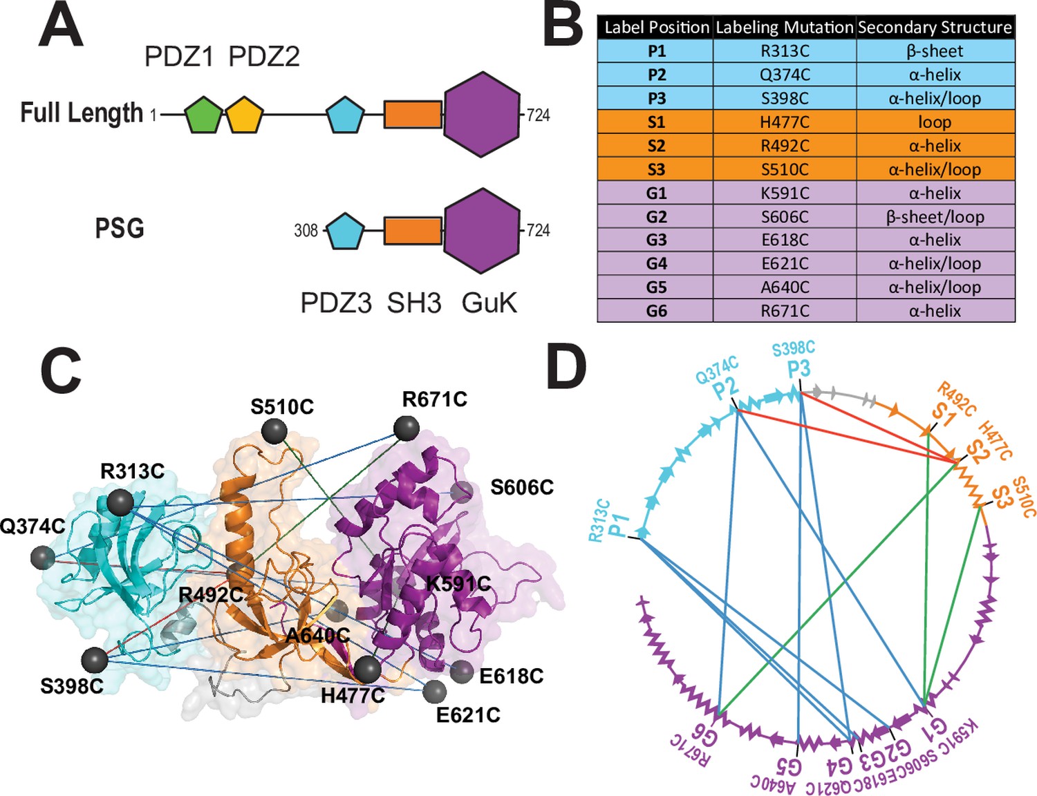
A FRET network to probe structure and dynamics in PSD-95.
(A) Schematic representation of the domain organization in PSD-95. (B) Cysteine substitutions used for fluorescent labeling. Label position indicates the domain for each mutant and the order in the primary sequence. Label mutation gives the residue identity. Secondary structure describes the local secondary structural environment at each site. (C) Location of the labeling sites within the supertertiary structure of the PSG fragment. The PSG is shown in cartoon representation with PDZ3 (cyan), SH3 (orange) and GuK (purple). Spheres indicate the location of the dye while lines indicate the experimental Förster resonance energy transfer (FRET) pairs. Although only the PSG is shown, measurements were made on full-length PSD-95. (D) Connectivity in the FRET network. The primary sequence of PSD-95 is shown in a circular representation with each domain colored as in panel C. The secondary structural elements are indicated: α helices (zig zag) and β sheets (arrows). The position of each labeling site is indicated by the domain and order in the primary sequence. The FRET pairs used for measurements are indicated by lines connecting the labeling sites used in that variant with FRET pairs spanning PDZ3-GuK (blue), PDZ3-SH3 (red), and SH3-GuK (green).
Figure 2
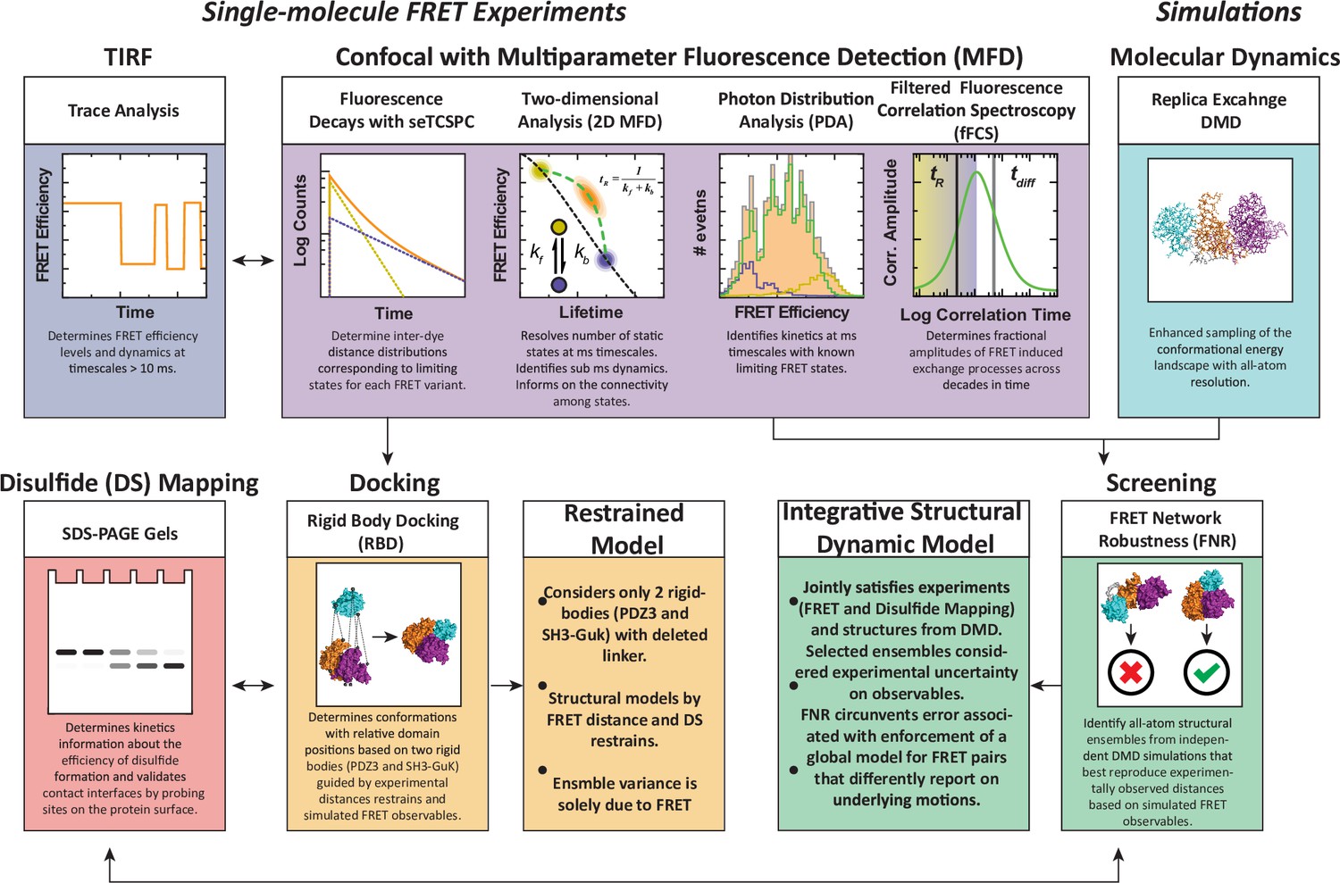
An experimental workflow for dynamic structural biology.
For single molecule Förster resonance energy transfer (smFRET) experiments, total internal reflection fluorescence (TIRF) and confocal modalities were used to probe the FRET network consisting of 12 complementary pairs of FRET labeling sites. Comparing the two approaches provides validation through the use of different dyes, sample preparation, instrumentation, and handling. Confocal smFRET with pulsed interleaved excitation and multiparameter fluorescence detection were holistically analyzed in four modalities, including fluorescence decay analysis, two-dimensional representations, photon distribution analysis, and filtered fluorescence correlation spectroscopy. Each approach provides complementary information on the underlying conformational distribution with respect to inter-dye distances and protein dynamics. For simulations: replica-exchange discrete molecular dynamics (rxDMD) provided an independent view of the energy landscape. For structural modeling: two approaches were used. Rigid body docking used two fixed structures (PDZ3 and SH3-GuK) to identify domain orientations that satisfied the FRET-derived interdye distances for all 12 FRET pairs, resulting in a fully FRET-restrained model. Screening of the rxDMD simulations with the FRET distances and the boundaries from FRET robustness analysis allowed classification of structures that mutually satisfy the simulated model (rxDMD) and the FRET observables. Finally, to validate the proposed structural models, we used disulfide mapping and probed interfaces corresponding to the preferred structural basins. In a refinement step, we introduced the disulfide information for both structural modeling approaches.
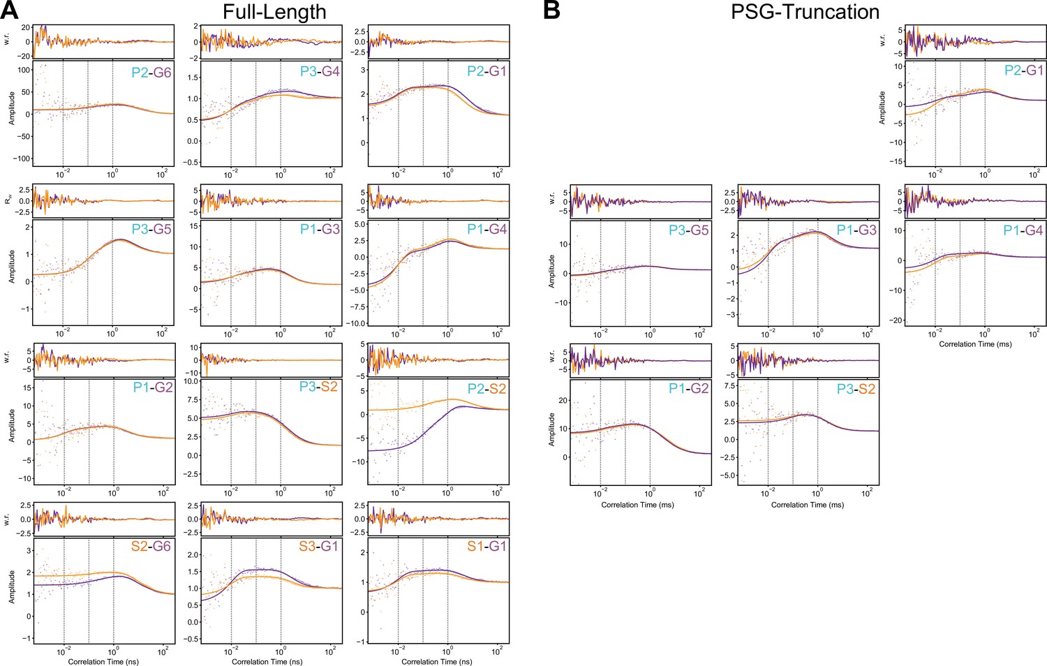
Figure 3
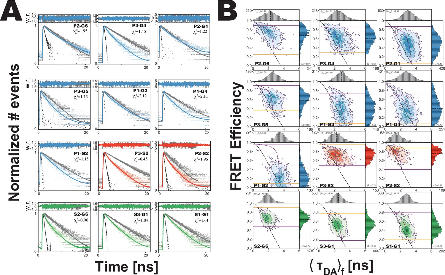
Analysis of confocal microscopy data.
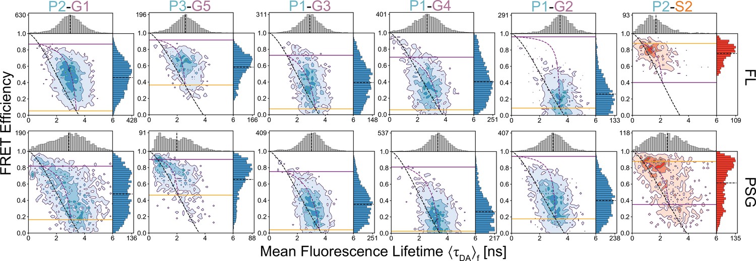
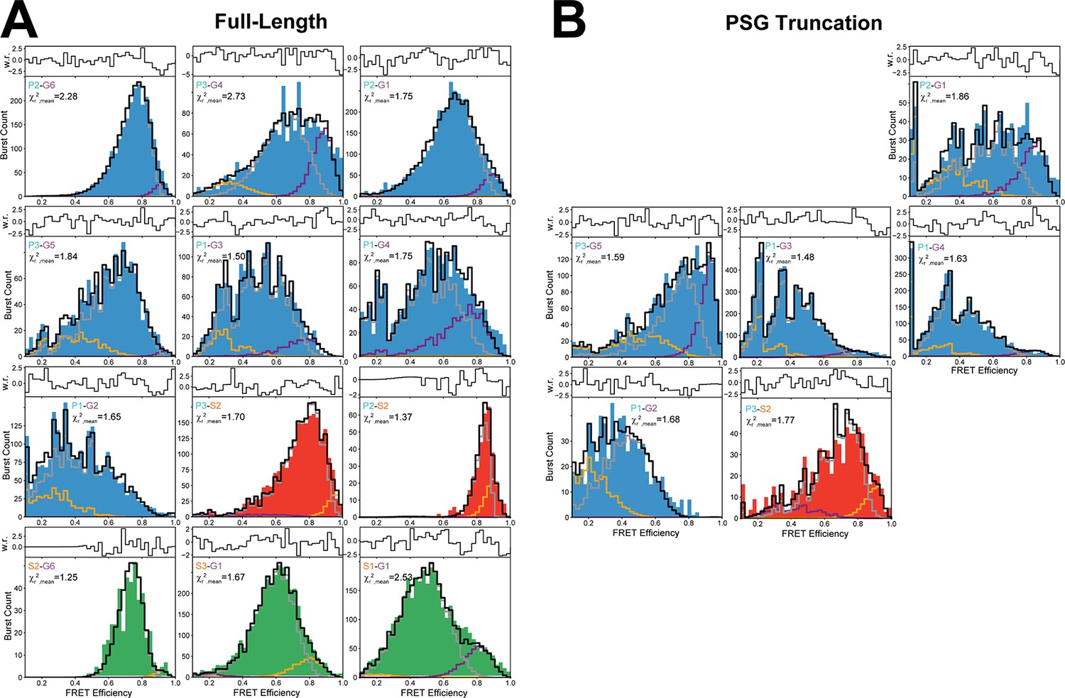
(A) Global fit of the Förster resonance energy transfer (FRET)-sensitized donor fluorescence decay curves for full length variants. Shown are subensemble time correlated single photon counting decays for FRET pairs spanning PDZ3-GuK (blue), PDZ3-SH3 (red), and SH3-GuK (green). The instrument response function is shown in black, and the donor-only fluorescence decay is shown in gray. Raw histogram data are shown as points, with fits overlaid as lines. FRET quenches donor fluorescence, which reduces the lifetime and introduces curvature into fluorescence decay. The presence of more than one underlying state with different FRET efficiencies results in multi-exponential fluorescence decays. Fit parameters can be found in Appendix 1—table 2 and Appendix 1—table 3. Details of the model and fit can be found in Materials and methods. (B) Multiparameter fluorescence histograms of full-length PSD-95 FRET variants. Multiparameter fluorescence detection histograms for FRET pairs spanning PDZ3-GuK (blue), PDZ3-SH3 (red), and SH3-GuK (green) as noted in each panel. Variant details can be found in Figure 1. Overlaid on the contour plots are the static FRET-lines (black, dashed), dynamic FRET-lines (purple, dashed), and solid horizontal lines corresponding to the limiting states A (orange) and B (purple) from seTCSPC. Also given are the burst-wise average values for the mean donor fluorescence lifetime () and mean FRET efficiency ( (black, dashed lines in 2D histograms). Dynamic exchange is immediately evident from broadening and skew rightward from the static FRET-line for each variant. Correction parameters for these histograms can be found in Appendix 1—table 2while parameters for the static and dynamic FRET-lines can be found in Appendix 1—table 5, Appendix 1—table 6, respectively.
Figure 4 with 4 supplements
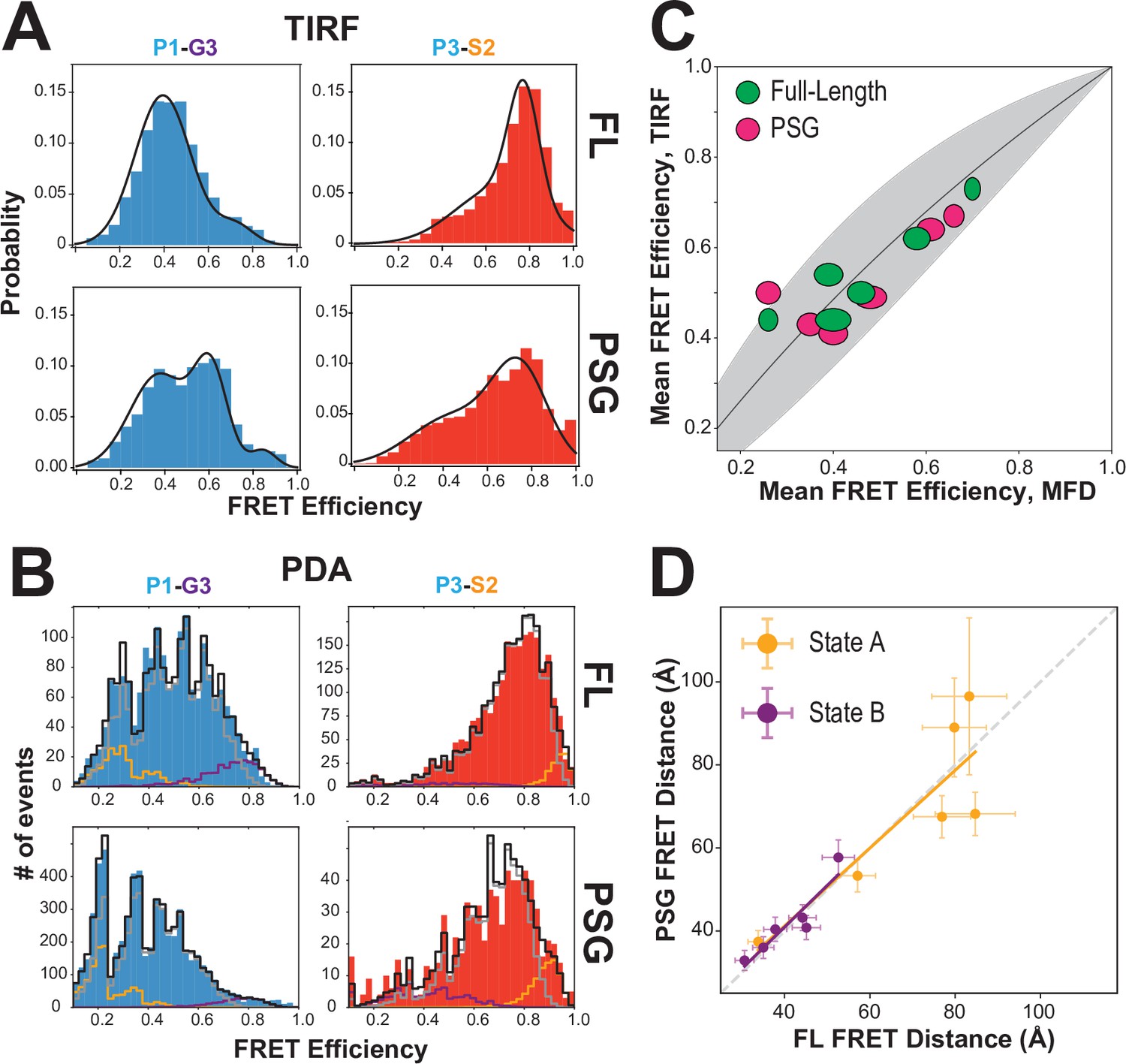
Effect of truncating PSD-95 on PSG supertertiary structure.
(A) Representative single-molecule total internal reflection fluorescence (smTIRF) Förster resonance energy transfer (FRET) efficiency histograms for full-length PSD-95 (top) and the corresponding truncated PSG fragment (bottom). Shown are variants P1-G3 (blue) and P3-S2 (red). (B) Representative PDA plots using a 2 ms time window for the same variants from panel A using the same coloring. Molecules occupying limiting states A and B are highlighted in orange and purple, respectively. (C) Comparison of mean FRET efficiency as measured with smTIRF (y-axis) and multiparameter fluorescence detection (MFD) (x-axis) for full-length (green) and PSG (pink) variants. Ellipse eccentricities represent the relative width of FRET distributions observed by each method. The expected relationship given the different fluorophores used is shown as a line with the shaded region corresponding to Förster radius uncertainty. Förster radii used were as used previously (McCann et al., 2012; Yanez Orozco et al., 2018). The fit to the ideal relationship gave = 2.13 with .=0.72 and = 1.42. (D) Comparison of the seTCSPC limiting-state distances for full-length PSD-95 (y-axis) and the PSG fragment (x-axis). Distances are shown for state A (orange; Slope = 0.94; Pearson Correlation Coefficient (Rp)=0.86) and state B (purple; Slope = 1.0; Rp = 0.93).
-
Figure 4—source data 1
This zip archive contains all of the FRET values for each variant measured with smTIRF.
The data is included as excel files for the accumulated per-frame (i.e. pointwise) FRET along with the time-averaged (per molecule) FRET for each selected molecule. Also included are the intensity time traces for representative molecules along with summary information about the number of molecules for each data panel.
- https://cdn.elifesciences.org/articles/77242/elife-77242-fig4-data1-v2.zip
Figure 4—figure supplement 1
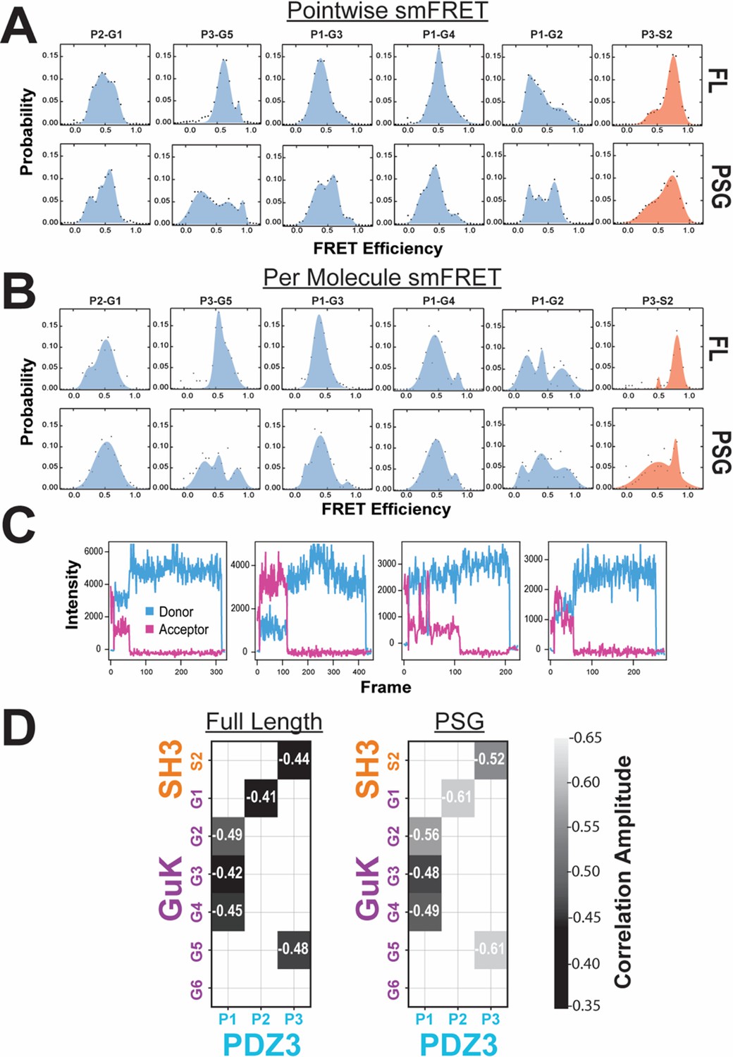
Effect of truncation on PSD-95 as measured with smTIRF.
(A) Population histograms of pointwise single-molecule total internal reflection fluorescence (smTIRF) data (per 100 millisecond frame) for variants with Förster resonance energy transfer (FRET) pairs spanning PDZ3-GuK (blue), PDZ3-SH3 (red) as indicated above each panel. Shown are data for full-length PSD-95 (top) and the truncated PSG (bottom). (B) Time-averaged (per molecule) population histograms from the same smTIRF data shown in panel A with identical coloring. (C) Representative single-molecule time traces for variant P2-G1 in the PSG truncation showing static and dynamic molecules. (D) Matrix representation of site-specific dynamics in full-length PSD-95 (left) and the PSG truncation (right). The axes specify the domains and labeling sites with each variant placed at the intersection between sites used. Shown are the mean Pearson correlation coefficients as calculated from smTIRF donor-acceptor time traces before photobleaching occurred. The Pearson correlation coefficients capture anticorrelated FRET transitions on the subsecond timescale such as those visible in panel C.
Figure 4—figure supplement 2
Comparison of multiparameter fluorescence histograms of PSG-truncated and full-length PSD-95 Förster resonance energy transfer (FRET) variants.
Multiparameter fluorescence detection (MFD) plots of PSG truncations (bottom). Full Length (FL) variants with same labeling sites are shown for comparison (top). The labeling sites are indicated within each panel. Dynamic lines and limiting states for PSG variants were determined from global fitting of donor fluorescence decays of PSG variants shown in Figure 3. Experimental parameters can be found in Appendix 1—table 3 and Appendix 1—table 4. Fit parameters for determination of the limiting states can be found in Appendix 1—table 3 and Appendix 1—table 4. Parameters for the calculation of static and dynamic FRET lines can be found in Appendix 1—table 5 and Appendix 1—table 6.
Figure 4—figure supplement 3
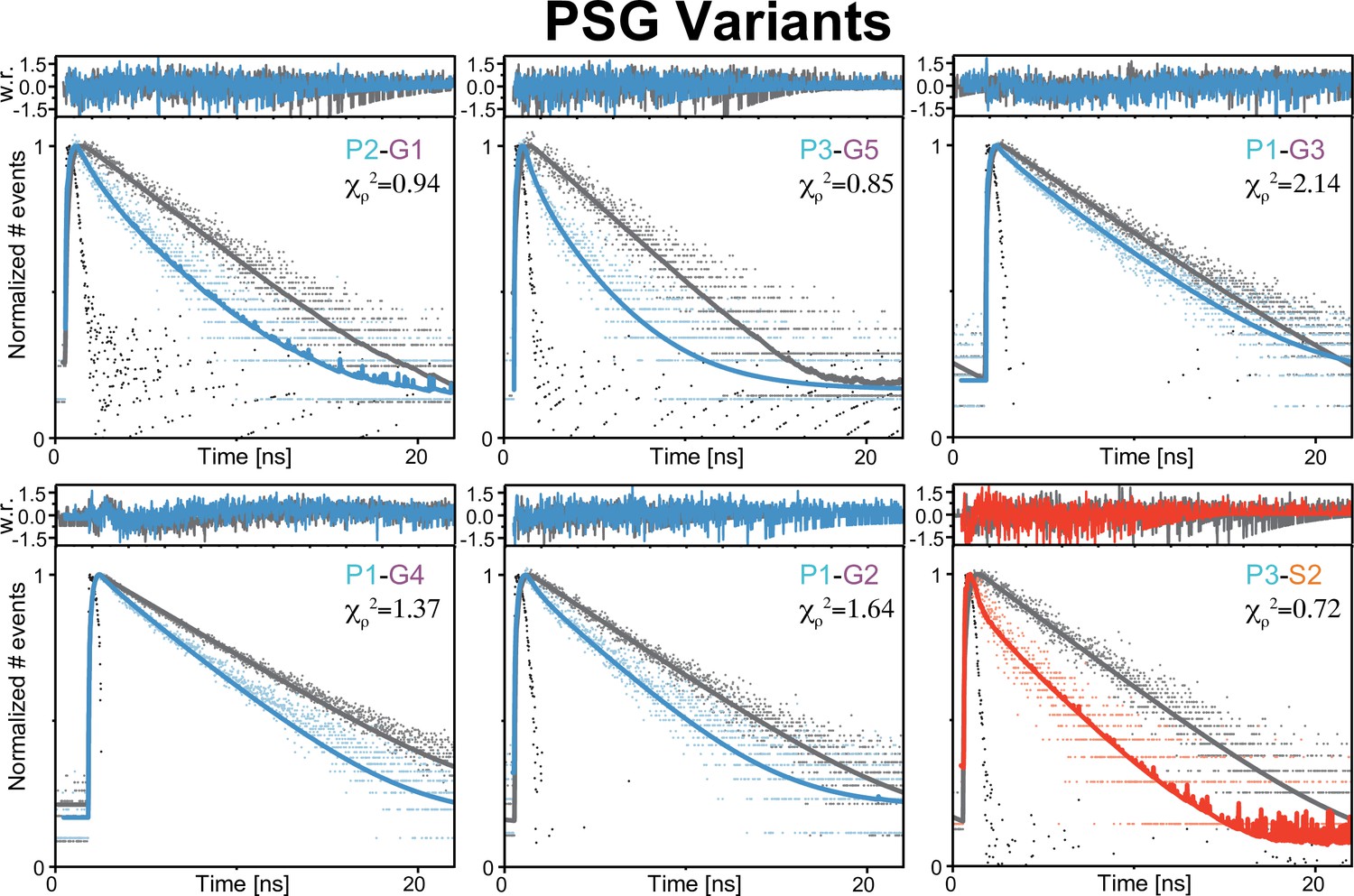
Global fit of seTCSPC Förster resonance energy transfer (FRET)-sensitized donor fluorescence decay curves for truncated PSG variants.
Fit parameters can be found in Appendix 1—table 3, Appendix 1—table 4. Fits are analogous to those shown in Figure 3 but for PSG variants donor only samples colored gray. FRET-sensitized donor decays colored blue for PDZ3-GuK; red for PDZ3-SH3.
Figure 4—figure supplement 4
Photon distribution analysis histograms.
Representative photon distribution analysis for both full length PSD-95 and PSG truncated variants. Data shown is binned using 2 ms time windows. Fits were performed globally with 1 ms, 2 ms, and 3 ms time windows for each sample. The displayed is the simple mean of for fits of all three time windows. Raw data is color coded as blue (PDZ3-GuK), red (PDZ3-SH3), or green (SH3-GuK). Data is binned using 50 evenly spaced bins in Förster resonance energy transfer (FRET) efficiency. Fits are shown in gray (dynamic fraction), orange (state A static fraction), purple (state B static fraction), and black (sum of three components). Fit parameters can be found in Appendix 2—table 1.
Figure 5 with 1 supplement
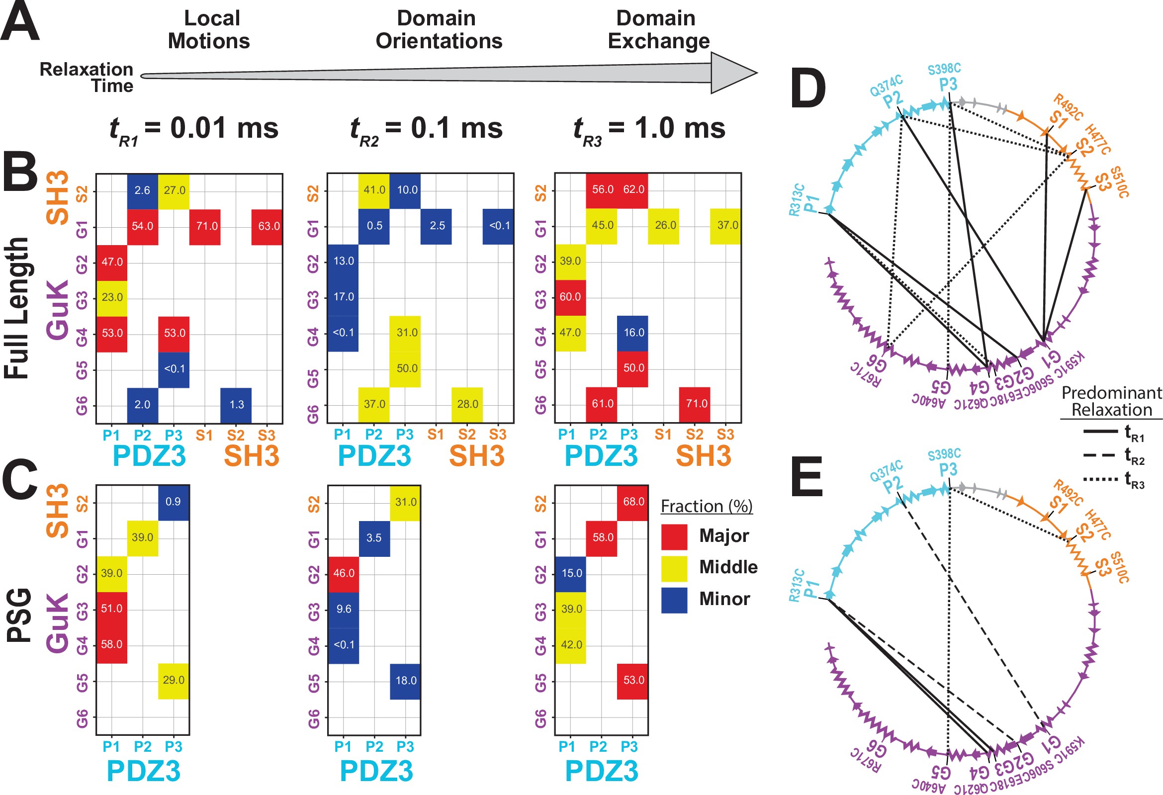
Effect of truncating PSD-95 on supertertiary dynamics within PSG.
Site-specific dynamics for each variant as measured with filtered fluorescence correlation spectroscopy (fFCS) and fit to a model with three correlation times at three decades in time from 10–5 s to 10–3 s. (A) Association between the dynamic relaxation time and the expected protein motions across the three decades in time used in the analysis. (B & C) Matrix representations of the relative contribution to dynamic relaxation at each decade in time (as indicated above the panel). The axes specify the domains and labeling sites with each variant placed at the intersection between sites used. In both panels, the relative contribution to relaxation at each timescale is highlighted: major (red); middle (yellow); minor (blue). The percentage is shown within each square. (B) Extent of dynamics across timescales for full length PSD-95. (C) Extent of dynamics across timescales for the PSG truncation, measured with the same variants. (D & E) The major contribution to dynamics is mapped onto the primary sequence. Shown are circular representations of the primary sequence with PDZ3 (cyan), SH3 (orange) and GuK (purple). The secondary structural elements are indicated: α helices (zig zag) and β sheets (arrows). Lines denote the fluorophore labeling sites for each measurement and indicate the predominant relaxation timescale: tR1 (solid); tR2 (dashed); tR3 (dotted). (D) Predominant timescale for relaxation of each FRET variant measured in full length PSD-95. (E) Predominant timescale for relaxation of each FRET variant measured in the PSG truncation. The most dominant relaxation times, tR1 and tR3, correspond to fast local motions and domain-scale conformational exchange, respectively.
Figure 5—figure supplement 1
Filtered fluorescence correlation spectroscopy fits.
(A) Cross-correlation curves for full-length PSD-95 variants as indicated within each panel. (B) Cross-correlation curves for truncated PSG variants as indicated within each panel. Curves were fit with diffusion timescales fit based on autocorrelation curves. Cross-correlation decay timescales are fixed to.01 ms,.10 ms, and 1.00 ms (gray, vertical dashes) such that relative amplitudes corresponding to each timescale can be directly compared (Figure 5). Weighted residuals are displayed in upper panels. Raw correlation data is shown as points with lines overlaid for fit curves. Purple data corresponds to low-Förster resonance energy transfer (FRET) to high-FRET component cross-correlation, while orange corresponds to low-FRET to high-FRET. Individual amplitudes are shared between the datasets, but each component is allowed a global scaling factor (Eqns. S2 and S3). Details of the model functions are available in Materials and methods.
Figure 6 with 4 supplements
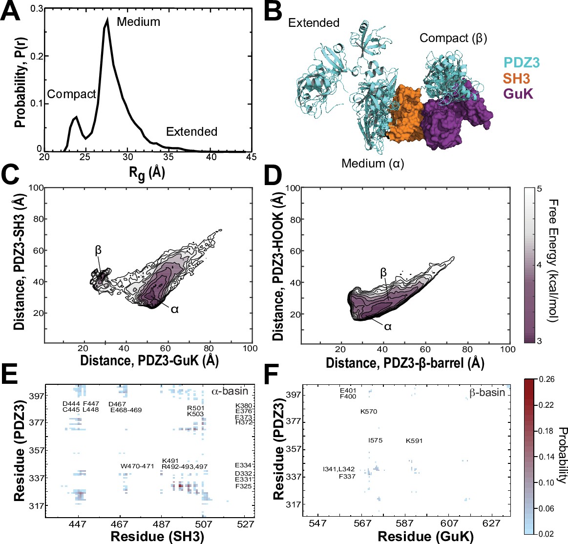
Discrete molecular dynamics of the PSG supramodule from PSD-95.
(A) Probability distribution of the radius of gyration (Rg) of the PSG during replica-exchange discrete molecular dynamics (DMD) simulations totaling 11.9 μs. (B) Representative conformations from the three basins apparent in the Rg distribution. The conformations and their respective population fractions in the highly sampled α-basin and less frequently sampled β-basin are provided in Figure 6—figure supplement 3. (C) 2D free energy landscape of the relative distance between centers of mass (COM) for PDZ3 and GuK (x-axis) or SH3 β-barrel (y-axis). (D) 2D free energy landscape of the relative distance between COM for PDZ3 and either the SH3 β-barrel (x-axis) or the SH3 HOOK insertion (y-axis). (E) Probability of pairwise residue contacts between PDZ3 and SH3, which define the α-basin. Residues from PDZ3 are on the y-axis while residues from SH3 are on the x-axis. (F) Probability of pairwise residue contacts between PDZ3 and GuK, which define the β-basin. Residues from PDZ3 are on the y-axis while residues from GuK are on the x-axis. The associated color bar indicates the normalized probability of the individual pairwise interactions.
Figure 6—figure supplement 1
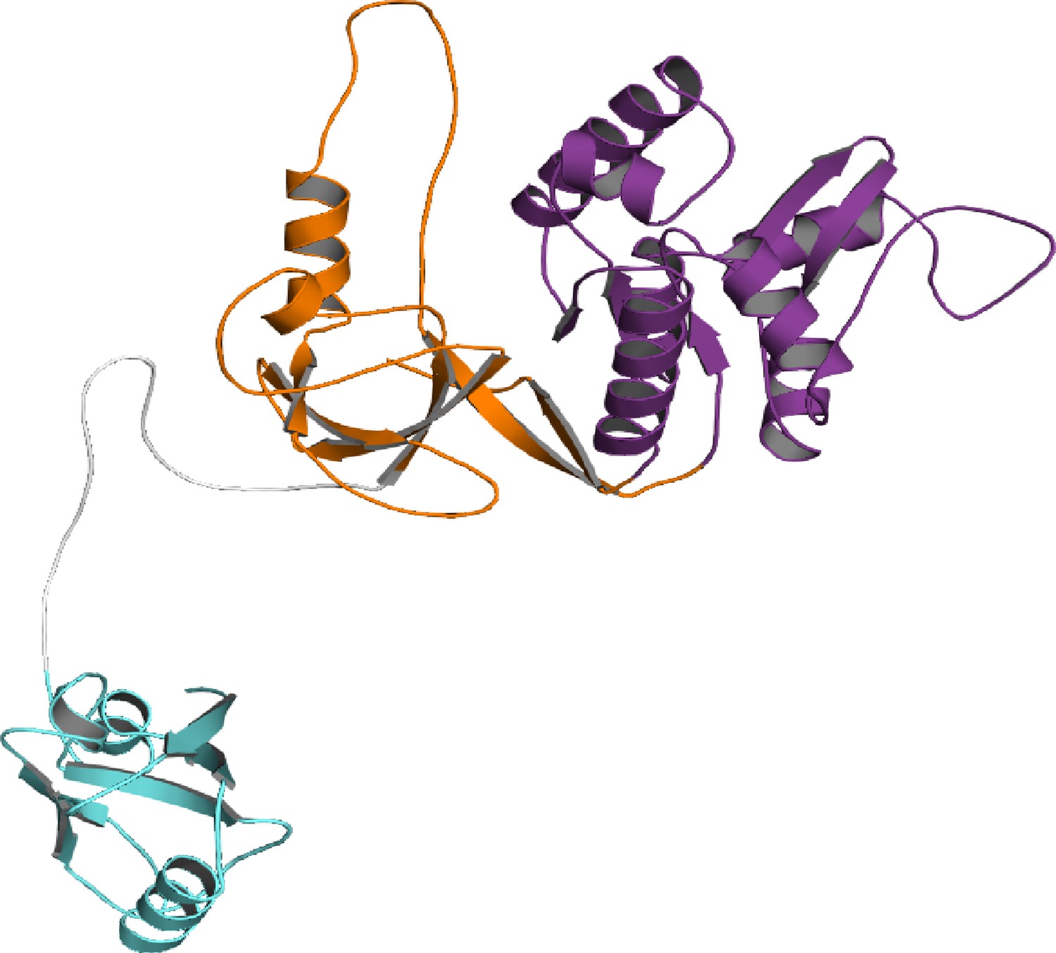
The starting conformation for the PSG supramodule from PSD-95 used in DMD simulations.
Cartoon representation of the initial model for discrete molecular dynamics (DMD) simulations showing PDZ3 (cyan), SH3 (orange) and GuK (purple). To avoid biasing the interactions, PDZ3 was positioned away from the SH3-GuK without any contacts. The model was constructed from the crystal structures of PDZ3 (1TP5) and SH3-GuK (1KJW). PDZ3 was placed in a random orientation without interdomain contacts to avoid bias. The PDZ3-SH3 linker and missing loops were reconstructed using our in-house loop reconstruction program ‘medusa-loop’.
Figure 6—figure supplement 2
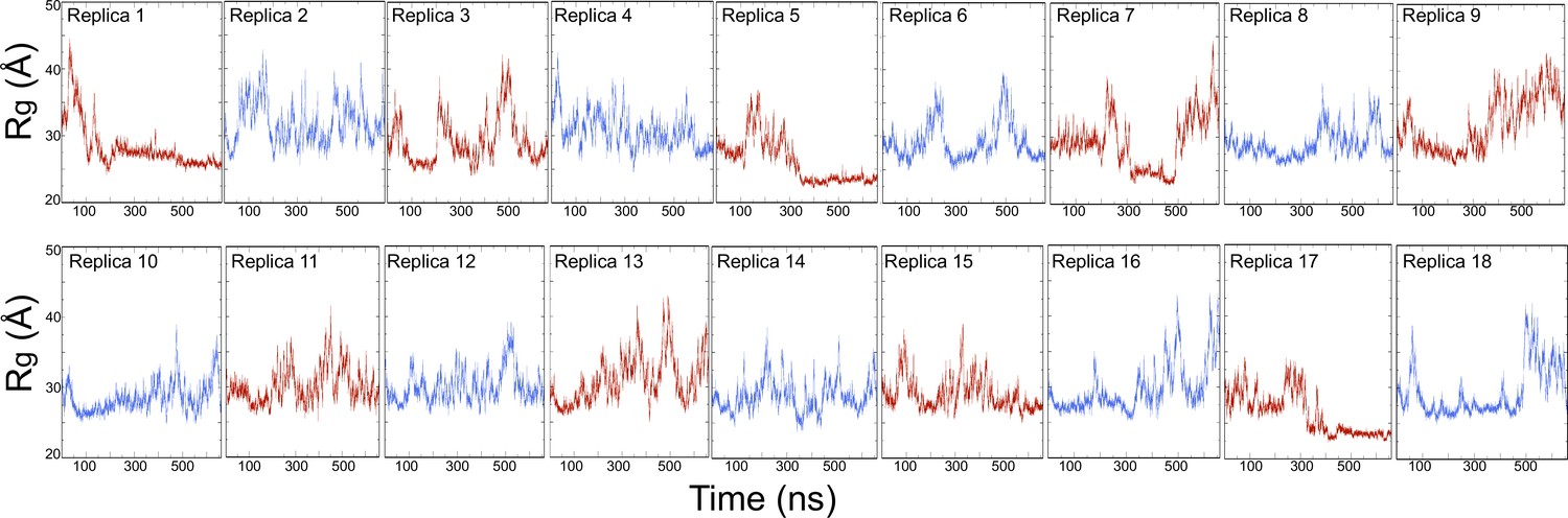
Time evolution of the radius of gyration (Rg) of PSG supramodule for 18 replicas discrete molecular dynamics (DMD) simulations.
The total simulation time for each replica is 660 ns and amounts to a total simulation time of 11.9 μs. We used the last 400 ns of replica exchange trajectories for the statistical analysis.
Figure 6—figure supplement 3
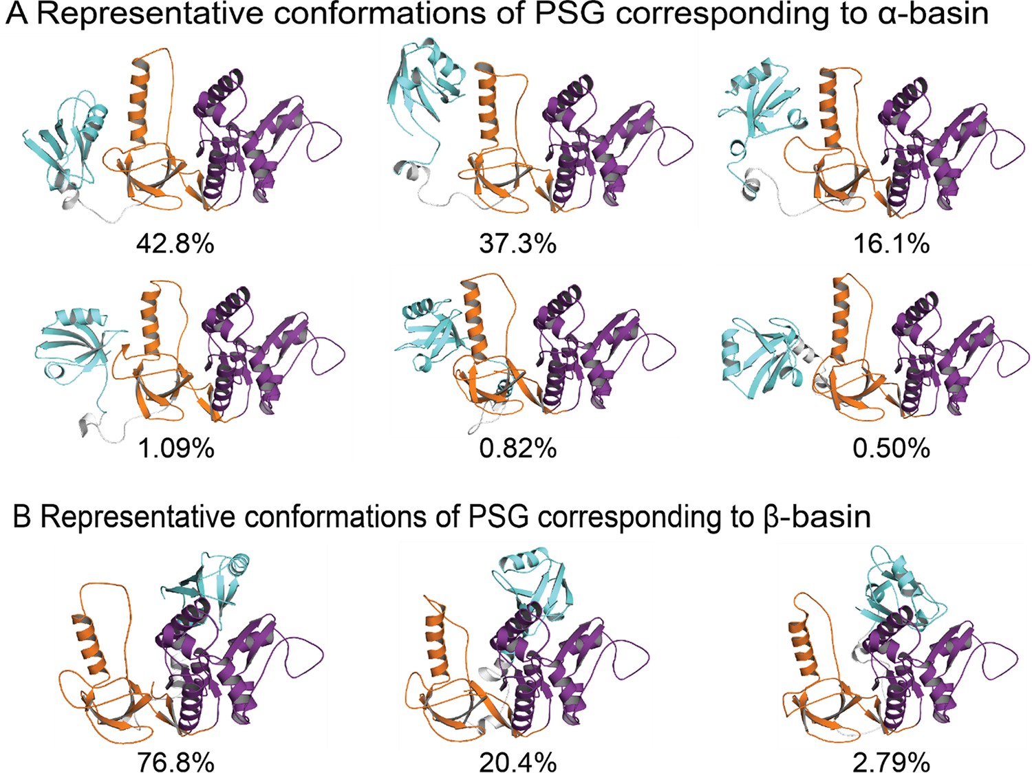
Representative conformations of PSG supramodule from PSD-95 (PDBDEV_00000164).
(A) Representative conformations and their population occupancy in the highly sampled α-basin with PDZ3 interacting with the SH3 domain. PDZ3 is colored cyan, SH3 colored orange, and GuK colored purple. A multiplicity of states is sampled within the fuzzy α-basin. The top centroid cluster in the α-basin shows PDZ3 to reorient away from the HOOK helix and sample the β1-β2 loop (RT loop in canonical SH3 domain). The pairwise contact maps from discrete molecular dynamics (DMD) show that interactions within the α-basin involved degenerate electrostatic interactions engaged by all conformations with occasional hydrophobic interactions leading an occluded PDZ3 binding pocket. (B) Representative conformations and their population in the β-basin with PDZ3 interacting with the GuK domain of PSG. The β-basin was comparatively well defined due to involvement of exposed hydrophobic residues in β3-α1 of PDZ3 and a relatively hydrophobic surface in GuK formed by α7, α5, and β10–11 (e.g. L349-F684, L342-L608), which support a limited range of conformations. Both basins infrequently engaged the canonical GLGF motif, which would prevent peptide binding to PDZ3. An RMSD cutoff of 8.0 Å was used to select the centroid clusters of α- and β-basins.
Figure 6—figure supplement 4

Comparison of equilibrated conformations observed in discrete molecular dynamics (DMD) to published crystal structures.
(A) Steric occlusion of the PDZ3 ligand-binding pocket within the α-basin. The structure of PDZ3 bound to a short peptide (1TP3, yellow) is aligned with PDZ3 from a representative α-basin model (cyan). The ligand is shown as a beta strand (yellow) that overlaps with the SH3 HOOK insertion (orange). (B) Lack of steric occlusion in the β-basin. The structure of GuK (yellow) bound to a MAP1A peptide (red) is aligned with a representative β-basin model (purple). The canonical ligand binding pockets of GuK and PDZ3 remain accessible in the β-basin.
Figure 7 with 2 supplements
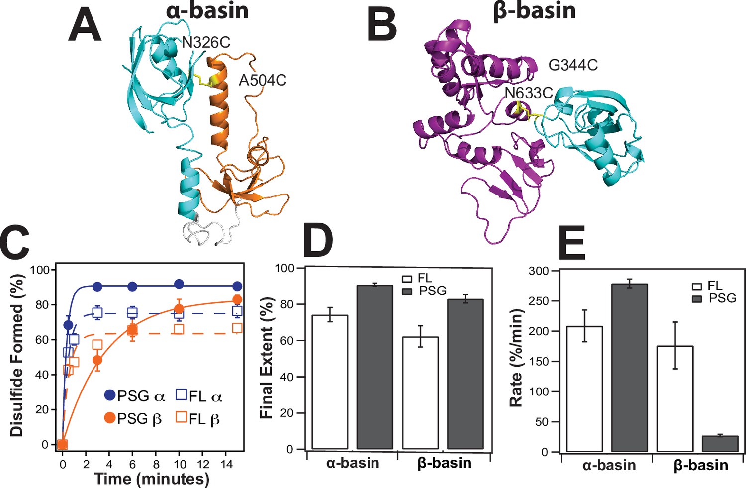
Disulfide mapping of the contact interfaces identified from DMD simulations.
Cartoon representations showing PDZ3 (cyan), SH3 (orange), and GuK (purple). (A) Target model from the α-basin. N326C-A504C disulfide in yellow. (B) Target model from the β-basin. G344C-N633C disulfide in yellow. (C) Kinetics of disulfide bond formation as measured using non-reducing SDS-PAGE (Figure 7—figure supplement 1) showing the α-basin (blue) and the β-basin (orange). Data for full-length PSD-95 are shown as circles with fits as solid lines while data for the PSG truncations is shown as open circles with dashed lines. (D) Final extent of disulfide bond formation from single exponential fits to the kinetic data for full-length PSD-95 (white) and the PSG truncation (gray). (E) Kinetic rate of disulfide bond formation from single exponential fits to the kinetic data. Error bars represent the SD from three replicate measurements.
Figure 7—figure supplement 1
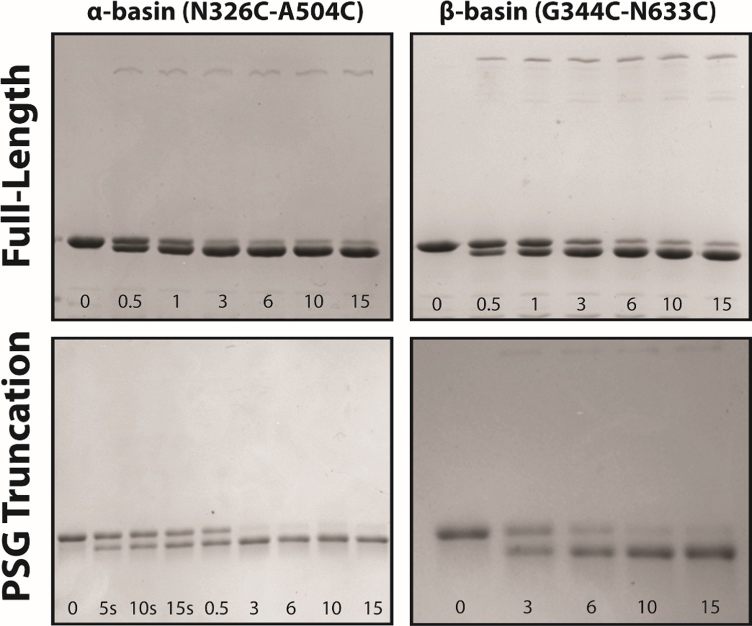
Disulfide mapping of the contact interfaces from DMD.
Representative non-reducing SDS-PAGE gels used to extract kinetic information about rates of disulfide formation. The top row shows 7.5% acrylamide gels for full-length PSD-95 variants. The bottom row shows 10% acrylamide gels used for PSG truncations. The variant and the introduced mutations are noted above each column. The time for each lane is indicated within each panel in minutes unless indicated otherwise. The background-subtracted intensity of each band was obtained using ImageJ to calculate the background-subtracted mean intensity, which are plotted in Figure 7. Each experiment was repeated in triplicate.
Figure 7—figure supplement 2
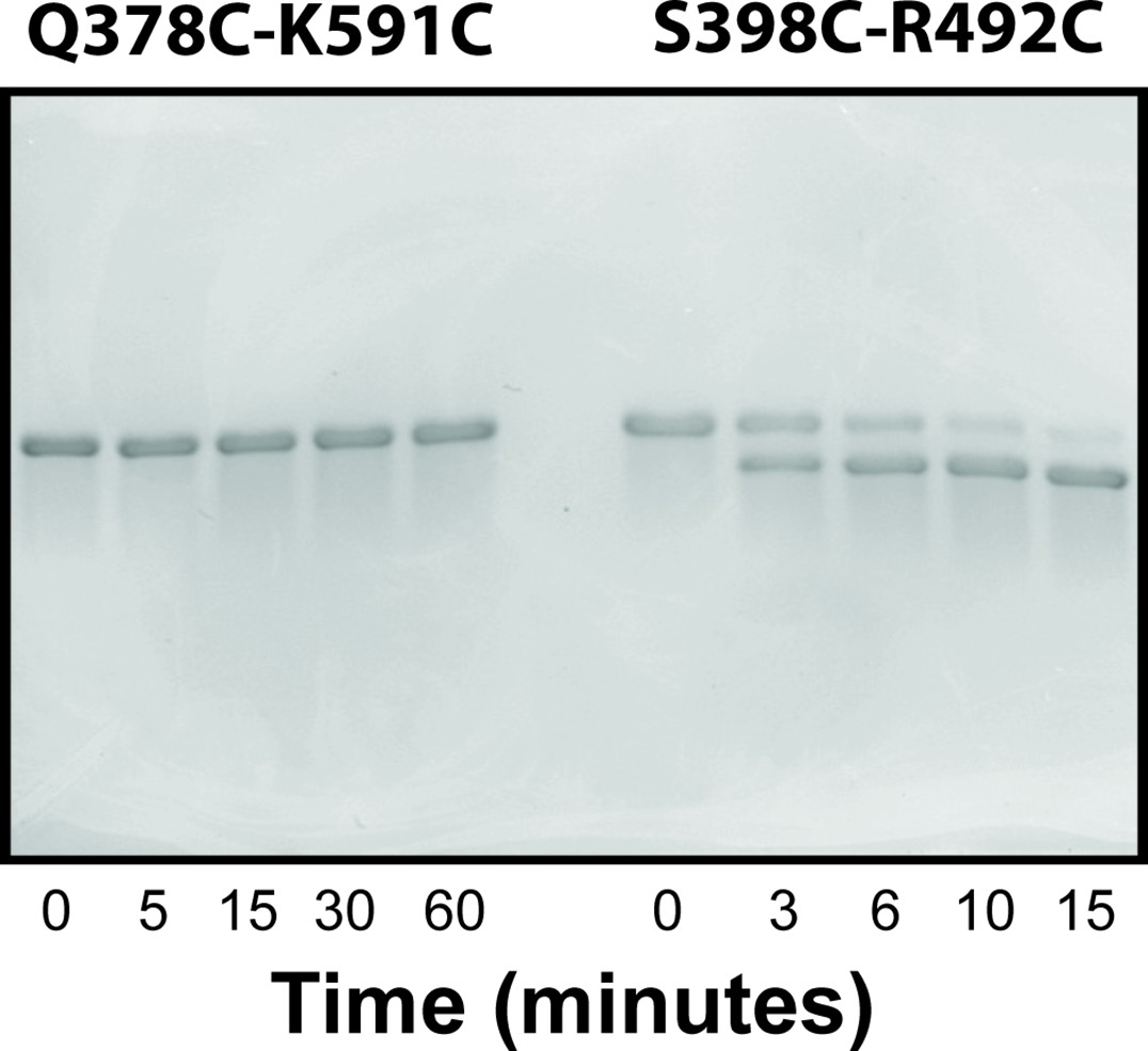
Controls for disulfide mapping of the contact interfaces from DMD.
Representative non-reducing SDS-PAGE using 10% acrylamide gels to probe for disulfide formation in selected Förster resonance energy transfer variants. The variant Q378-K591 residue pair is not predicted to be in contact as part of either conformational basin. In contrast, the S398-R492 residue pair does occasionally sample close distances in the α-basin. The experiments used PSG truncations with the introduced mutations as noted above each experiment. The time for each lane is indicated beneath the panel in minutes.
Figure 8 with 2 supplements
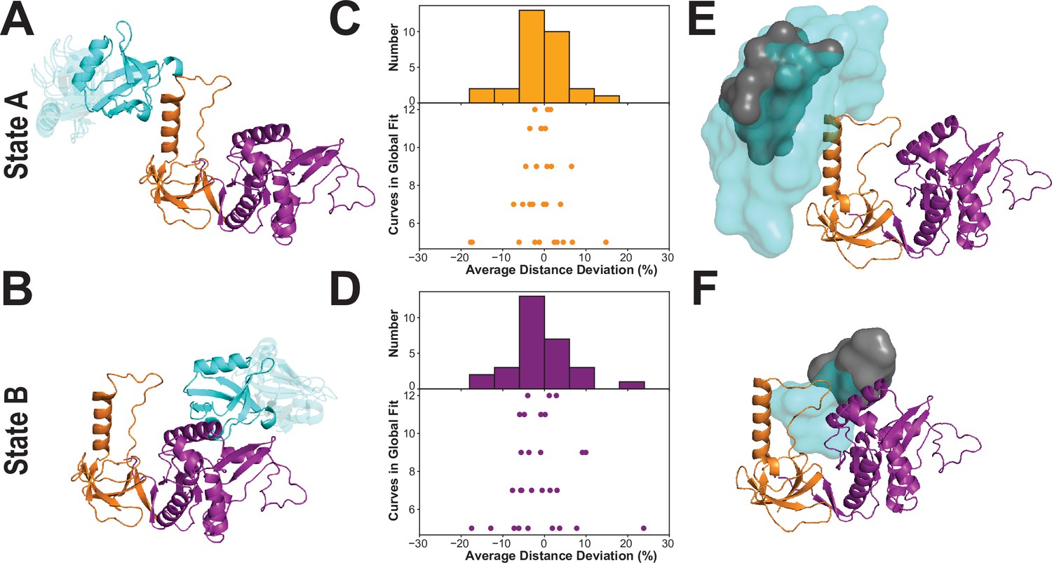
Modeling the supertertiary structural ensemble with experimental FRET restraints.
(A & B) Cartoon representations of the best fit models from rigid body docking of PDZ3 based on the FRET distances with PDZ3 (cyan), SH3 (orange) and GuK (purple) (PDBDEV_00000161). (A) Best fit model for full-length PSD-95 in limiting state A. (B) Best fit model for limiting state B. (C & D) FRET network robustness analysis. We randomly selected sub-samples of the FRET network and repeated a global fit on the reduced FRET network. Histograms show the percent error in distance for all sub-sample fits relative to the global fit. Distance errors from each sub-sample fit are shown beneath the histogram as a function of the number of variants included. Distances and associated widths resulting from subsampled global fitting are summarized in Appendix 4—table 2. (C) Average distance deviation for state A from global fitting of individual sub-sampled FRET networks. (D) Average distance deviation for state B. The histograms show that the distributions are centered on the reported distances regardless of the number of variants. These summary statistics indicate convergence toward the center of the distribution as the number of samples globally fit is increased. (E & F) Heterogeneity of the conformational state ensembles based on classification of structures from discrete molecular dynamics (DMD). The position of PDZ3 in each model is represented as a sphere at its center of mass. The gray surfaces represent the 95% confidence intervals for localization of the PDZ3, based on the F-test for the ratio of χ2r for all docking structures relative to the χ2r of the top-ranked structure with nine free parameters (number of distances used for docking of PDZ3). This captures the uncertainty in distances from the global fit but not the full heterogeneity of each basin. The cyan surfaces represent conformational space accessible to PDZ3 within the thresholds from the FRET network robustness analysis shown in panels C and D (Appendix 4—table 2) (PDBDEV_00000164). (E) Fuzziness of the conformational α-basin related to state A. (F). Fuzziness of the conformational β-basin related to state B.
Figure 8—figure supplement 1
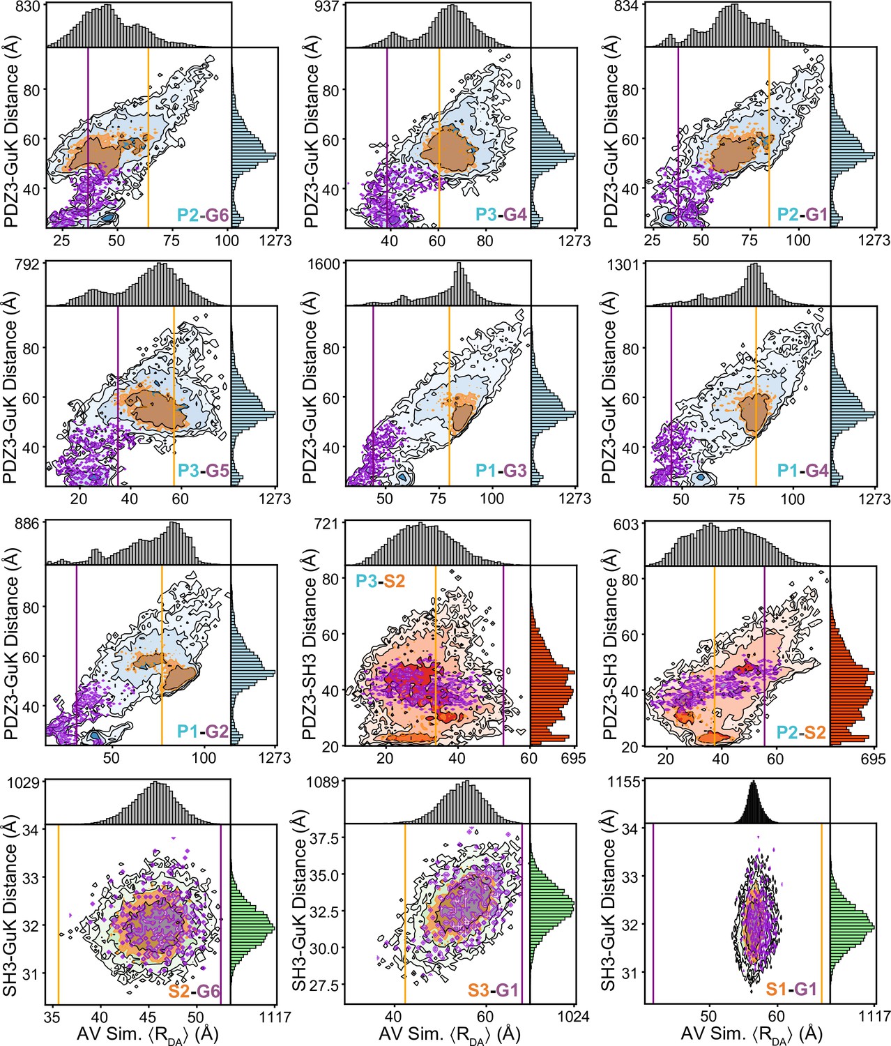
Responsiveness of individual variants to the underlying conformational distribution.
Shown are the simulated interdye distances from accessible volume (AV) simulations using discrete molecular dynamics (DMD) structures. The 20,871 snapshot structures from DMD were used to calculate the AV for the dyes at each labeling position, which were then used to calculate average interdye distances for each snapshot structure. These interdye distances for each variant are plotted against the distance between centers of mass (CoM) for the relevant domains. These 2D plots provide a qualitative analysis of how each Förster resonance energy transfer (FRET) pair reflects changes in the underlying conformation. The limiting state distances for each variant are shown as vertical lines for state A (orange) and state B (purple). Overlaid are contours corresponding to DMD structures residing in state A (orange) and state B (purple), which are within the distance uncertainty from sub-sampling analysis of TCSPC fluorescence decays and the AV simulation distances. For most variants, limiting state distances qualitatively agree with the locations of local maxima in the simulated interdye distance distributions. However, some variants show both maxima along the same vertical line indicating that the conformational dynamics are not fully captured by that FRET pair. Furthermore, presence of FRET pairs spanning SH3-GuK show the most difference between simulated and measured distances, likely owing to the limited dynamics of these domains in silico.
Figure 8—figure supplement 2
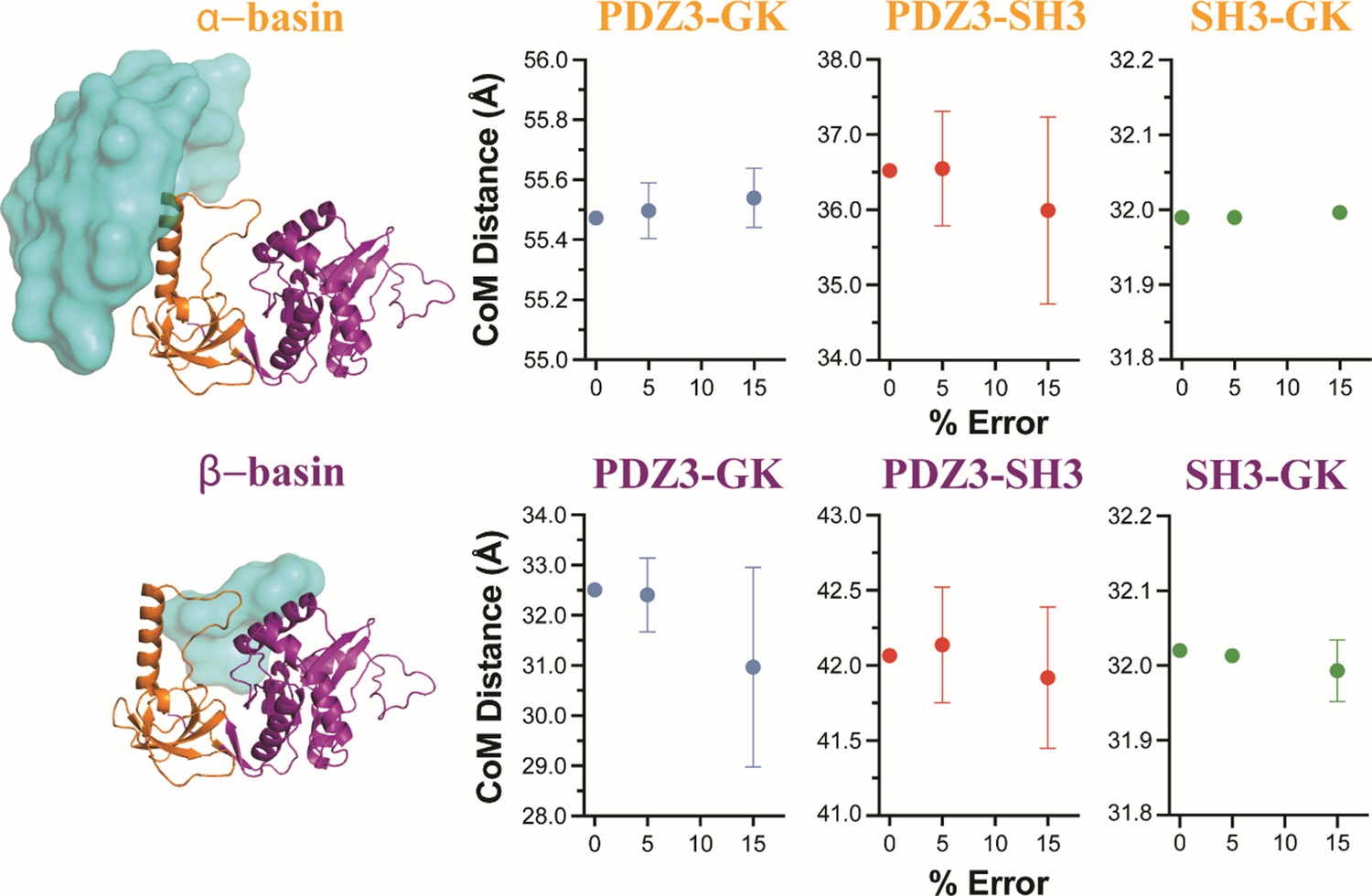
Model robustness analysis.
As with the Förster resonance energy transfer (FRET) network robustness analysis, where we analyzed the model dependence on the inclusion of individual variants, here we bootstrapped the dependency of the models on error in the FRET distances using the same framework. For each trial, we introduced a random, artificial error on each of the FRET distances and repeated the classification of structures from discrete molecular dynamics (DMD) into the two basin ensembles. To check the dependence on the magnitude of the error, we used introduced a random error to each variant between 5 and –5% or between 15 and –15% of the original distance. Each condition was repeated three times with different random errors. To compare conditions, we measured the change in the center of mass of the surface distribution composed from the individual PDZ3 centers of mass identified by that screen. We found that increasing the distance error did not significantly impact the classification of structures into the two ensembles. The variance in the mean ensemble positions over three repeats increased with increasing error along with small shifts in the mean positions. Notably,+/-15% is greater than the uncertainties in distances obtained via global fitting of fluorescence decays, suggesting that the intrinsic uncertainty in the FRET-derived distances from a single fit (Appendix 4—table 2) does not significantly impact the ensemble assignment or their fuzziness.
Figure 9 with 2 supplements

Energy landscape for the conformational ensemble of the PSG supramodule within PSD-95.
(A) Energy landscape surface from principal component analysis (Figure 9—figure supplement 1). The basins α and α’ correspond to the two sub-basins separated by a small shoulder along principal component 2. The surface was rescaled such that the integrated volumes of basins α and β matched the experimental population fractions from global analysis of the lifetime decays for states A and B, respectively. The transitions and their associated timescales were taken from correlation analysis. The timescale for each transition is indicated by colored arrows. The fastest transitions are associated with local motions, which were not resolved by Förster resonance energy transfer but are inferred from discrete molecular dynamics (DMD) simulations and filtered fluorescence correlation spectroscopy (fFCS). (B) Conformational exchange within the energy landscape. Cartoon models for the PSG supramodule in each basin are shown with PDZ3 (cyan), SH3 (orange) and GuK (purple). The timescale for each transition is indicated by colored arrows as in panel A. The movie in Figure 9—video 1 illustrate the supertertiary dynamics of the PSG supramodule. Structures were sampled from the the ensmbles to PDB-Dev ( PDBDEV_00000164) .
Figure 9—figure supplement 1

Principal component analysis of COM and AV data.
In order to visualize the conformational landscape of the PSG supramodule within PSD95, we performed principal component analysis using the distances between the domain’s centers of mass (COM) and the simulated for PDZ3 to SH3 and PDZ3 to GuK (Figure 8—figure supplement 1). Data were analyzed using scikit-learn (sklearn) in Python. Data were first standardized such that each set of inter-COM and AV-derived interdye distances had mean 0 and unit variance using the sklearn.preprocessing.StandardScaler. Principal components were calculated using sklearn.decomposition.PCA with two components. The surface depth corresponds to the relative number of structures from discrete molecular dynamics (DMD) simulations which occupy some region of the principal component (PC) space. PCA results in basins α and β separated along PC1, which explains 65% of the standardized dataset variance. The variance along PC2 (16% explained variance ratio) mostly corresponds to apparent heterogeneity in basin α. Additionally, there is an apparent saddle point corresponding to the transition pathway between the two basins along PC1. This suggests that the motions corresponding to heterogeneity in basin α are distinct from those corresponding to interdomain transitions as observed by Förster resonance energy transfer. This surface was rescaled for Figure 9 such that the integrated volume of the two basins were equivalent to the population fractions for states A and B obtained from seTCSPC analysis.
Figure 9—video 1
Illustration of supertertiary dynamics of the PSG supramodule within PSD-95.
The movie was constructed using 100 frames from ensembles A and B generated using FNR analysis (all shown structures are included in PDBDEV_00000164). To represent experimental population fractions from experiments with full-length PSD-95, the movie shows 46 total frames sampled from state A and 54 from state B, with dwell times of 23 frames in A and 27 in B, respectively.
Figure 10 with 1 supplement
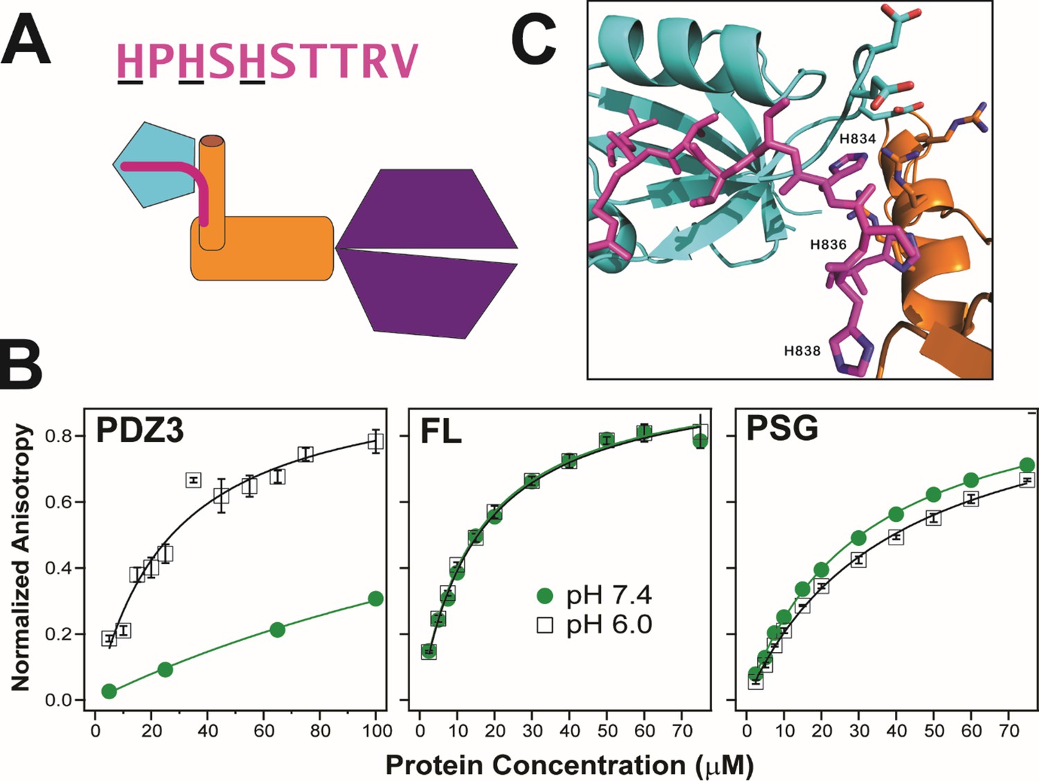
Effect of supertertiary environment on neuroligin binding.
(A) Schematic illustration of the interaction between PSD-95 and the neuroligin peptide (pink). The sequence of the neuroligin C-terminal peptide used in binding experiments is shown with pH-sensitive histidines underlined. (B) Representative binding isotherms for the neuroligin peptide binding to truncated PDZ3 (left), full-length PSD-95 (middle) and truncated PSG (right). Shown are data at pH 7.4 (green circles) and pH 6.0 (open squares). Anisotropy values were normalized relative to the final anisotropy taken from non-linear least squares fits (lines). Error bars represent the standard deviation from three replicate measurements. (C) Representative conformation from docking of the neuroligin peptide (pink) to PSG in the α–basin from discrete molecular dynamics (DMD) (Figure 10—figure supplement 1). The peptide C-terminus interacts with the GLGF motif in PDZ3 (cyan). Charged residue interactions between PDZ3 and SH3 (orange) prevent electrostatic repulsion of histidines that otherwise weakens peptide binding at neutral pH.
Figure 10—figure supplement 1
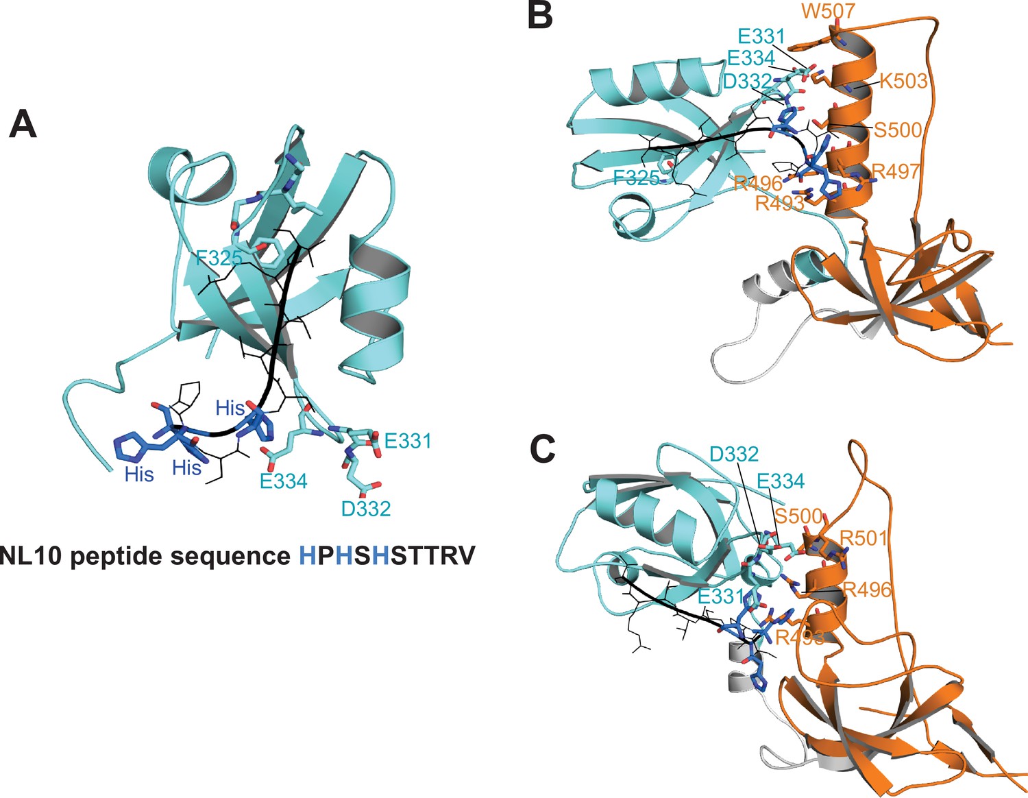
Docking of neuroligin to PDZ3 and the PSG supramodule in α-basin.
(A) Docked conformation of NL10 peptide bound to the PDZ3. The NL10 peptide is shown in black with the three histidine residues shown in blue. When protonated, these histidine residues extend towards E331, D332, and E334 in PDZ3, which may explain the higher binding affinity at low pH. At physiological pH, the negatively charged residues will inhibit binding of uncharged histidines. (B–C) Representative conformations of NL10 peptide binding to PDZ3 within the PSG α-basin. In the context of PSG, positively charged residues in the SH3 HOOK insertion form salt-bridges with the negatively charged residues in PDZ3. These electrostatic interactions sequester these negative charges to stabilize the binding of NL10 at physiological pH.
Tables
Table 1
Fit statistics for models with increasing numbers of states.
The fit parameter χ2r,seTCSPC is shown for each variant when fit to a model with an increasing number of structural states as indicated above each column. Increasing from one to two states results in a significant increase in fit quality. Further increase to three states provides little to no improvement in fit quality. Increasing model complexity beyond two states decreases the average fit quality. Details of variants can be found in Figure 1.
| Sample | One State χ2r,seTCSPC | Two State χ2r,seTCSPC | Three State χ2r,seTCSPC |
|---|---|---|---|
| P2-G6 | 8.46 | 2.54 | 1.95 |
| P3-G4 | 3.32 | 1.49 | 1.67 |
| P2-G1 | 1.66 | 1.22 | 1.53 |
| P3-G5 | 1.55 | 1.13 | 1.45 |
| P1-G3 | 2.86 | 2.12 | 2.38 |
| P1-G4 | 2.87 | 2.11 | 2.31 |
| P1-G2 | 1.54 | 1.15 | 1.52 |
| P3-S2 | 0.68 | 0.45 | 0.65 |
| P2-S2 | 14.65 | 1.96 | 1.58 |
| S2-G6 | 1.77 | 0.92 | 1.23 |
| S3-G1 | 5.75 | 1.84 | 1.78 |
| S1-G1 | 2.94 | 1.61 | 1.71 |
| Average | 4.00 | 1.55 | 1.65 |
Appendix 1—table 1
Details for MFD instruments used in this study.
Correction parameters for MFD that are specified for each experimental setup. The setup used to measure each variant is indicated in Appendix 1—table 2. HHU stands for Heinrich Heine University.
| Parameter | Setup 1 (Clemson) | Setup 2 (HHU) |
|---|---|---|
| Det. Efficiency Ratio (G/R) | 3.7 | 0.8 |
| Green Power (485 nm) | 80 µW | 60 µW |
| Red Power (640 nm) | 32 µW | 10 µW |
| PIE Repetition Rate | 20 MHz | 32 MHz |
| Repetition Time | 50.00 ns | 31.25 ns |
| Direct Acceptor Excitation, δ | 2.2 | 1.3 |
| Spectral Crosstalk, G→R, α | 1.7 | 1.7 |
Appendix 1—table 2
Correction parameters for multiparameter fluorescence detection.
Correction parameters determined for each FRET variant based on buffer measurements for backgrounds, donor-only and directly-excited acceptor fluorescence for quantum yields (QYG, QYR), and standard stock fluorophore solutions for G-factors. Parameters constant for all samples measured on a given setup are summarized at the end. Details of variants can be found in Figure 1 and Table 1. HHU stands for Heinrich Heine University.
| FL Variant | QYG | QYR | BGG(D) (kHz) | BGR(D) (kHz) | BGR(A) (kHz) | G-factor | Setup |
|---|---|---|---|---|---|---|---|
| P2-G6 | 0.72 | 0.26 | 0.85 | 0.45 | 0.30 | 1.06 | HHU |
| P3-G4 | 0.75 | 0.53 | 0.54 | 0.21 | 0.38 | 1.06 | HHU |
| P2-G1 | 0.72 | 0.38 | 0.53 | 0.18 | 0.17 | 0.83 | Clemson |
| P3-G5 | 0.77 | 0.46 | 0.51 | 0.16 | 0.17 | 0.83 | Clemson |
| P1-G3 | 0.71 | 0.37 | 0.38 | 0.14 | 0.15 | 0.83 | Clemson |
| P1-G4 | 0.76 | 0.39 | 0.41 | 0.15 | 0.15 | 0.83 | Clemson |
| P1-G2 | 0.75 | 0.37 | 0.54 | 0.20 | 0.19 | 0.83 | Clemson |
| P3-S2 | 0.81 | 0.43 | 0.50 | 0.16 | 0.17 | 0.83 | Clemson |
| P2-S2 | 0.68 | 0.26 | 0.78 | 0.45 | 0.36 | 1.06 | HHU |
| S2-G6 | 0.70 | 0.26 | 0.74 | 0.39 | 0.29 | 1.06 | HHU |
| S3-G1 | 0.71 | 0.44 | 0.51 | 0.26 | 0.40 | 1.06 | HHU |
| S1-G1 | 0.73 | 0.49 | 0.51 | 0.26 | 0.40 | 1.06 | HHU |
| PSG Variant | QYG | QYR | BGG(D) (kHz) | BGR(D) (kHz) | BGR(A) (kHz) | G-factor | Setup |
| P2-G1 | 0.72 | 0.31 | 0.56 | 0.18 | 0.17 | 0.83 | Clemson |
| P3-G5 | 0.72 | 0.35 | 0.51 | 0.16 | 0.17 | 0.83 | Clemson |
| P1-G3 | 0.74 | 0.40 | 0.38 | 0.14 | 0.15 | 0.83 | Clemson |
| P1-G4 | 0.69 | 0.39 | 0.41 | 0.15 | 0.15 | 0.83 | Clemson |
| P1-G2 | 0.75 | 0.35 | 0.53 | 0.19 | 0.17 | 0.83 | Clemson |
| P3-S2 | 0.77 | 0.38 | 0.50 | 0.16 | 0.17 | 0.83 | Clemson |
Appendix 1—table 3
Fit parameters from seTCSPC using a Two State Model.
| FL Variant | Donor Fraction | Scattering Amplitude | τD(0) | <κ2> | rD|D,∞ | rA|A,∞ | rA|D,∞ | Species Fraction xI | Species Fraction xII | τD(A),xI | τD(A),xII | τD(A),fI | τD(A),fII | χ,seTCSPC2 |
|---|---|---|---|---|---|---|---|---|---|---|---|---|---|---|
| P2-G6 | 0.02 | 0.07 | 3.60 | 0.72 | .09 | .14 | .07 | 0.46 | 0.54 | 2.73 | 0.39 | 2.78 | 0.65 | 2.54 |
| P3-G4 | 0.00 | 0.17 | 3.76 | 0.82 | .18 | .14 | .08 | 0.46 | 0.54 | 2.67 | 0.53 | 2.75 | 0.83 | 1.49 |
| P2-G1 | 0.01 | 0.04 | 3.59 | 0.85 | .14 | .19 | <.01 | 0.46 | 0.54 | 3.41 | 0.46 | 3.41 | 0.74 | 1.22 |
| P3-G5 | 0.15 | 0.12 | 3.86 | 0.85 | .14 | .21 | .02 | 0.46 | 0.54 | 2.45 | 0.33 | 2.57 | 0.59 | 1.13 |
| P1-G3 | 0.39 | 0.09 | 3.56 | 0.83 | .19 | .13 | .01 | 0.46 | 0.54 | 3.31 | 0.97 | 3.31 | 1.25 | 2.12 |
| P1-G4 | 0.11 | 0.05 | 3.79 | 0.89 | .15 | .22 | .08 | 0.46 | 0.54 | 3.58 | 1.13 | 3.58 | 1.41 | 2.11 |
| P1-G2 | 0.00 | 0.05 | 3.77 | 0.83 | .12 | .20 | .04 | 0.46 | 0.54 | 3.44 | 0.15 | 3.45 | 0.34 | 1.15 |
| P3-S2 | 0.02 | 0.0 | 4.04 | 0.88 | .19 | .25 | .02 | 0.46 | 0.54 | 0.28 | 2.09 | 0.37 | 2.27 | 0.45 |
| P2-S2 | 0.00 | 0.20 | 3.38 | 0.71 | .04 | .20 | .04 | 0.46 | 0.54 | 0.41 | 2.03 | 0.67 | 2.14 | 1.96 |
| S2-G6 | 0.00 | 0.16 | 3.50 | 0.72 | .11 | .13 | <.01 | 0.46 | 0.54 | 0.33 | 1.80 | 0.58 | 1.97 | 0.92 |
| S3-G1 | 0.00 | 0.20 | 3.56 | 0.77 | .14 | .05 | .01 | 0.46 | 0.54 | 0.80 | 2.95 | 1.09 | 2.98 | 1.84 |
| S1-G1 | 0.00 | 0.12 | 3.64 | 0.79 | .18 | .14 | .09 | 0.46 | 0.54 | 2.96 | 0.76 | 2.99 | 1.06 | 1.61 |
| PSG Variant | Donor Fraction | Scattering Amplitude | τD(0) | κ2 | rD|D,∞ | rA|A,∞ | rA|D,∞ | Species Fraction xI | Species Fraction xII | τD(A),xI | τD(A),xII | τD(A),fI | τD(A),fII | χr,se TCSPC2 |
| P2-G1 | 0.00 | 0.09 | 3.60 | 0.79 | .14 | .08 | .07 | 0.52 | 0.49 | 3.01 | 0.65 | 3.03 | 0.94 | 0.94 |
| P3-G5 | 0.04 | 0.10 | 3.59 | 0.85 | .14 | .25 | .02 | 0.52 | 0.49 | 1.93 | 0.36 | 2.09 | 0.62 | 0.85 |
| P1-G3 | 0.11 | 0.06 | 3.72 | 0.84 | .19 | .16 | .01 | 0.52 | 0.49 | 3.57 | 0.92 | 3.57 | 1.22 | 2.14 |
| P1-G4 | 0.05 | 0.06 | 3.46 | 0.87 | .14 | .25 | .07 | 0.52 | 0.49 | 3.38 | 0.66 | 3.38 | 0.94 | 1.37 |
| P1-G2 | 0.00 | 0.06 | 3.77 | 0.83 | .14 | .18 | .04 | 0.52 | 0.49 | 3.12 | 0.23 | 3.14 | 0.45 | 1.64 |
| P3-S2 | 0.05 | 0.07 | 3.87 | 0.86 | .14 | .25 | .04 | 0.52 | 0.49 | 0.47 | 2.52 | 0.77 | 2.62 | 0.72 |
Appendix 1—table 4
Interdye distances from the global fit of seTCSPC decays.
Distances resulting from seTCSPC fits. Model details are in Materials and Methods. All R0 for distance calculations taken as 52 Å, state widths set to 6 Å. Model fit parameters can be found in Appendix 1—table 3. Details of variants can be found in Figure 1 and Table 1. Uncertainties corresponding to 95% confidence intervals were estimated using the F-test for the ratio of χr,seTCSPC2 of the final fit to the χr,seTCSPC2 under variation of each parameter independently. The number of degrees of freedom was 2663 for all curves (number of data points-number of parameters).
| FL Variant | (Å) | (Å) |
|---|---|---|
| P2-G6 | 64.0±2.0 | 36.6±4.4 |
| P3-G4 | 60.4±2.9 | 38.5±1.1 |
| P2-G1 | 84.7±7.0 | 37.8±3.8 |
| P3-G5 | 57.1±3.2 | 35.0±6.0 |
| P1-G3 | 79.8±9.8 | 44.2±8.3 |
| P1-G4 | 83.3±5.2 | 45.1±5.8 |
| P1-G2 | 76.9±7.4 | 30.6±4.5 |
| P3-S2 | 33.8±6.0 | 52.6±2.1 |
| P2-S2 | 37.4±3.5 | 55.6±1.6 |
| S2-G6 | 35.6±3.4 | 52.5±1.4 |
| S3-G1 | 42.3±2.8 | 67.8±4.2 |
| S1-G1 | 66.5±2.9 | 41.7±2.1 |
| FL Fraction | 46.1% | 53.9% |
| PSG Variant | 〈RDA,A〉(Å) | 〈RDA,B〉(Å) |
| P2-G1 | 68.2±6.2 | 40.4±7.6 |
| P3-G5 | 53.3±3.0 | 36.0±5.5 |
| P1-G3 | 89.0±10.5 | 43.2±4.3 |
| P1-G4 | 96.5±12.0 | 40.8±2.0 |
| P1-G2 | 67.5±2.1 | 32.9±3.5 |
| P3-S2 | 37.4±3.9 | 57.7±5.7 |
| PSG Fraction | 51.8% | 48.2% |
Appendix 1—table 5
Parameters for calculation of static FRET-lines in MFD plots.
The static FRET-lines are calculated using these parameters and shown for visual reference in MFD plots in Figure 3 and Figure 4—figure supplement 2. FRET-lines are corrected for dynamic averaging due to fluorophore linker dynamics via polynomials relating the species fluorescence lifetimes, τD(A),x, from seTCSPC fits and linker-movement corrected apparent fluorescence-averaged fluorescence decay lifetimes, τD(A),f. These polynomials take the form: . Polynomial coefficients are determined via simulations of state widths in the Margarita software package. Static FRET-lines describe the expected relationship between and FRET efficiency for non-dynamic populations as is varied from 0 to the donor-only lifetime. Values for are listed in Appendix 1—table 3. Details of variants can be found in Figure 1 and Table 1. The static FRET-lines take the form: .
| FL Variant | p0 | p1 | p2 | p3 | p4 |
|---|---|---|---|---|---|
| P2-G6 | –0.020 | 0.362 | 0.465 | –0.109 | 0.008 |
| P3-G4 | –0.020 | 0.368 | 0.442 | –0.099 | 0.007 |
| P2-G1 | –0.020 | 0.362 | 0.466 | –0.109 | 0.008 |
| P3-G5 | –0.021 | 0.372 | 0.430 | –0.094 | 0.006 |
| P1-G3 | –0.019 | 0.361 | 0.471 | –0.111 | 0.008 |
| P1-G4 | –0.021 | 0.369 | 0.438 | –0.098 | 0.007 |
| P1-G2 | –0.020 | 0.369 | 0.441 | –0.099 | 0.007 |
| P3-S2 | –0.022 | 0.378 | 0.407 | –0.086 | 0.005 |
| P2-S2 | –0.018 | 0.353 | 0.500 | –0.124 | 0.009 |
| S2-G6 | –0.019 | 0.358 | 0.481 | –0.115 | 0.008 |
| S3-G1 | –0.019 | 0.361 | 0.471 | –0.111 | 0.008 |
| S1-G1 | –0.020 | 0.364 | 0.459 | –0.106 | 0.008 |
| PSG Variant | p0 | p1 | p2 | p3 | p4 |
| P2-G1 | –0.020 | 0.362 | 0.465 | –0.109 | 0.008 |
| P3-G5 | –0.020 | 0.362 | 0.466 | –0.109 | 0.008 |
| P1-G3 | –0.020 | 0.367 | 0.448 | –0.102 | 0.007 |
| P1-G4 | –0.019 | 0.357 | 0.486 | –0.118 | 0.009 |
| P1-G2 | –0.020 | 0.369 | 0.441 | –0.099 | 0.007 |
| P3-S2 | –0.021 | 0.372 | 0.427 | –0.093 | 0.006 |
Appendix 1—table 6
Parameters for calculation of dynamic FRET-lines in MFD plots.
The dynamic FRET-lines are calculated using these parameters and shown for visual reference in MFD plots in Figure 3 and Figure 4—figure supplement 2. Two-State dynamic FRET-lines describe the path in FRET efficiency vs plots on which populations exhibiting fractional mixing between two limiting, Gaussian-distributed states would fall. Dynamic lines are corrected like static lines for linker dynamics. Lifetimes for limiting states are taken from seTCSPC analysis (Figure 3A and Appendix 1—table 3). Details of variants can be found in Figure 1 and Table 1. Dynamic FRET-lines take the form: .
| Variant | p0 | p1 | p2 | p3 |
|---|---|---|---|---|
| P2-G6 | –2.499 | 1.894 | 0.000 | 0.000 |
| P3-G4 | –2.134 | 1.768 | 0.000 | 0.000 |
| P2-G1 | –2.608 | 1.767 | 0.000 | 0.000 |
| P3-G5 | –2.653 | 2.023 | 0.000 | 0.000 |
| P1-G3 | –1.355 | 1.400 | 0.000 | 0.000 |
| P1-G4 | –1.482 | 1.414 | 0.000 | 0.000 |
| P1-G2 | –4.946 | 2.435 | 0.000 | 0.000 |
| P3-S2 | –3.337 | 2.453 | 0.000 | 0.000 |
| P2-S2 | –1.984 | 1.907 | 0.000 | 0.000 |
| S2-G6 | –2.118 | 2.049 | 0.000 | 0.000 |
| S3-G1 | –1.675 | 1.560 | 0.000 | 0.000 |
| S1-G1 | –1.763 | 1.586 | 0.000 | 0.000 |
| Variant | p0 | p1 | p2 | p3 |
| P2-G1 | –1.955 | 1.641 | 0.000 | 0.000 |
| P3-G5 | –2.146 | 2.003 | 0.000 | 0.000 |
| P1-G3 | –1.713 | 1.479 | 0.000 | 0.000 |
| P1-G4 | –2.014 | 1.597 | 0.000 | 0.000 |
| P1-G2 | –3.712 | 2.179 | 0.000 | 0.000 |
| P3-S2 | –2.247 | 1.844 | 0.000 | 0.000 |
Appendix 2—table 1
Reaction rates and population fractions from Photon Distribution Analysis (PDA).
| FL Variant | kAB (ms–1) | kBA (ms–1) | kR (ms–1) | TR (ms) | Static Fraction A (%) | Static Fraction B (%) | Kinetic Fraction (%) |
|---|---|---|---|---|---|---|---|
| P2-G6 | 4.10 | 3.15 | 7.25 | 0.14 | 0.4 | 4.3 | 95.3 |
| P3-G4 | 3.08 | 2.99 | 6.07 | 0.17 | 9.8 | 25.2 | 65.0 |
| P2-G1 | 4.76 | 3.56 | 8.32 | 0.12 | 1.4 | 8.1 | 90.5 |
| P3-G5 | 1.97 | 5.76 | 7.73 | 0.13 | 19.4 | 1.3 | 83.1 |
| P1-G3 | 4.53 | 7.00 | 11.53 | 0.09 | 25.0 | 8.0 | 67.1 |
| P1-G4 | 3.25 | 4.75 | 8.00 | 0.13 | 0.0 | 25.1 | 74.9 |
| P1-G2 | 0.72 | 8.11 | 8.83 | 0.11 | 27.7 | 0.4 | 72.0 |
| P3-S2 | 5.54 | 3.14 | 8.68 | 0.12 | 6.5 | 3.2 | 90.3 |
| P2-S2 | 2.00 | 7.03 | 9.03 | 0.11 | 27.8 | 1.0 | 71.2 |
| S2-G6 | 7.32 | 5.01 | 12.33 | 0.08 | 2.9 | 0.0 | 97.1 |
| S3-G1 | 5.19 | 6.76 | 11.95 | 0.08 | 11.2 | 2.2 | 86.6 |
| S1-G1 | 3.52 | 5.84 | 9.36 | 0.11 | 1.7 | 14.2 | 84.1 |
| PSG Variant | kAB (ms–1) | kBA (ms–1) | kR (ms–1) | TR (ms) | Static Fraction A (%) | Static Fraction B (%) | Kinetic Fraction (%) |
| P2-G1 | 5.09 | 10.80 | 15.89 | 0.06 | 35.4 | 19.2 | 45.4 |
| P3-G5 | 4.10 | 7.65 | 11.75 | 0.09 | 23.7 | 26.3 | 50.0 |
| P1-G3 | 5.28 | 15.90 | 21.18 | 0.05 | 35.0 | 3.3 | 61.7 |
| P1-G4 | 3.27 | 16.20 | 19.47 | 0.05 | 26.4 | 2.9 | 70.7 |
| P1-G2 | 2.91 | 28.80 | 31.71 | 0.03 | 35.8 | 0.1 | 64.1 |
| P3-S2 | 7.32 | 4.23 | 11.55 | 0.09 | 11.0 | 13.6 | 75.4 |
Appendix 3—table 1
Fit parameters from global analysis of filtered Fluorescence Correlation Spectroscopy (fFCS).
Cross-correlation decay times were fixed for all samples, and their amplitudes were set as global parameters when fitting the cross-correlation curves. The average and log-space average, diffusion time (tdiff.) and geometric factor s are also global fit parameters as defined in Materials and Methods. Details of variants can be found in Figure 1 and Table 1. Decay timescales correspond to tR and amplitudes to CCi in Materials and Methods.
| FL Variant | 0.01ms Amplitude | 0.10ms Amplitude | 1.00ms Amplitude | Average | tdiff. (ms) | S |
|---|---|---|---|---|---|---|
| P2-G6 | 0.02 | 0.37 | 0.61 | 0.65 | 8.64 | 4.70 |
| P3-G4 | 0.53 | 0.31 | 0.16 | 0.20 | 10.19 | 4.70 |
| P2-G1 | 0.54 | 0.01 | 0.45 | 0.46 | 2.27 | 4.42 |
| P3-G5 | 0.00 | 0.50 | 0.50 | 0.55 | 4.47 | 4.42 |
| P1-G3 | 0.23 | 0.17 | 0.60 | 0.62 | 0.91 | 4.42 |
| P1-G4 | 0.53 | 0.00 | 0.47 | 0.47 | 1.08 | 4.42 |
| P1-G2 | 0.47 | 0.13 | 0.39 | 0.41 | 2.05 | 4.42 |
| P3-S2 | 0.27 | 0.10 | 0.62 | 0.64 | 0.91 | 4.42 |
| P2-S2 | 0.03 | 0.41 | 0.56 | 0.60 | 7.03 | 4.70 |
| S2-G6 | 0.01 | 0.28 | 0.71 | 0.74 | 9.74 | 4.70 |
| S3-G1 | 0.63 | 0.00 | 0.37 | 0.37 | 1.21 | 4.70 |
| S1-G1 | 0.71 | 0.03 | 0.26 | 0.27 | 2.10 | 4.70 |
| PSG Variant | 0.01ms Amplitude | 0.10ms Amplitude | 1.00ms Amplitude | Average | tdiff. (ms) | S |
| P2-G1 | 0.39 | 0.03 | 0.58 | 0.59 | 1.04 | 4.42 |
| P3-G5 | 0.29 | 0.18 | 0.53 | 0.55 | 0.79 | 4.42 |
| P1-G3 | 0.51 | 0.10 | 0.39 | 0.41 | 1.54 | 4.42 |
| P1-G4 | 0.58 | 0.00 | 0.42 | 0.43 | 0.80 | 4.42 |
| P1-G2 | 0.39 | 0.46 | 0.15 | 0.20 | 3.12 | 4.42 |
| P3-S2 | 0.01 | 0.31 | 0.68 | 0.72 | 0.96 | 4.42 |
Appendix 3—table 2
Variant-specific fit parameters for analysis of filtered Fluorescence Correlation Spectroscopy (fFCS).
The baseline/no-correlation parameter B, average number of bright molecules in the confocal volume N, and long-timescale decay amplitude (ATl for tL = 5.00 ms, accounts for long-timescale photophysical effects). Parameters correspond to low-FRET to high-FRET cross-correlation (LH), high-FRET to low-FRET cross-correlation (HL), low-FRET autocorrelation (LL), or high-FRET autocorrelation (HH). Details of variants can be found in Figure 1 and Table 1. Parameter definitions can be found in Materials and Methods.
| FL Variant | bLH | NB,LH | ATl,LH | bHL | NB,HL | ATl,HL | bLL | NB,LL | ATl,LL | bHH | NB,HH | ATl,HH |
|---|---|---|---|---|---|---|---|---|---|---|---|---|
| P2-G6 | 1.00 | 0.03 | 0.00 | 1.00 | 0.04 | 0.00 | 1.00 | 0.03 | 0.00 | 1.00 | 0.01 | 0.00 |
| P3-G4 | 1.02 | 37.23 | 0.59 | 1.02 | 4.85 | 0.01 | 1.02 | 0.06 | 0.78 | 1.02 | 0.03 | 0.89 |
| P2-G1 | 1.14 | 0.57 | 0.00 | 1.14 | 0.34 | 0.41 | 1.24 | 0.05 | 0.19 | 1.09 | 0.15 | 0.03 |
| P3-G5 | 1.03 | 1.10 | 0.12 | 1.03 | 0.96 | 0.23 | 1.01 | 0.06 | 0.27 | 1.00 | 0.21 | 0.20 |
| P1-G3 | 1.00 | 0.12 | 0.02 | 1.00 | 0.11 | 0.00 | 1.00 | 0.05 | 0.00 | 1.00 | 0.02 | 0.00 |
| P1-G4 | 1.24 | 0.20 | 0.06 | 1.24 | 0.26 | 0.00 | 1.32 | 0.06 | 0.00 | 1.20 | 0.01 | 0.00 |
| P1-G2 | 1.05 | 0.16 | 0.12 | 1.05 | 0.18 | 0.00 | 1.28 | 0.02 | 0.12 | 1.05 | 0.03 | 0.00 |
| P3-S2 | 1.35 | 0.14 | 0.06 | 1.35 | 0.10 | 0.29 | 1.45 | 0.03 | 0.00 | 1.50 | 0.05 | 0.00 |
| P2-S2 | 1.00 | 0.32 | 0.01 | 1.00 | 0.78 | 0.00 | 1.00 | 0.02 | 0.00 | 1.00 | 0.16 | 0.00 |
| S2-G6 | 1.00 | 0.82 | 0.00 | 1.00 | 0.95 | 0.00 | 1.00 | 0.43 | 0.00 | 1.00 | 0.51 | 0.00 |
| S3-G1 | 1.00 | 1.49 | 0.00 | 1.00 | 0.90 | 0.00 | 1.00 | 0.06 | 0.00 | 1.00 | 0.05 | 0.00 |
| S1-G1 | 1.00 | 1.99 | 0.00 | 1.00 | 1.20 | 0.21 | 1.00 | 0.05 | 0.04 | 1.00 | 0.05 | 0.04 |
| PSG Variant | BLH | NLH | ATl,LH | BHL | NHL | ATl,HL | BLL | NLL | ATl,LL | BHH | NHH | ATl,HH |
| P2-G1 | 1.05 | 0.09 | 0.57 | 1.05 | 0.12 | 0.00 | 1.11 | 0.01 | 0.00 | 1.03 | 0.04 | 0.00 |
| P3-G5 | 1.25 | 0.19 | 0.31 | 1.25 | 0.16 | 0.37 | 1.85 | 0.01 | 0.01 | 1.15 | 0.04 | 0.00 |
| P1-G3 | 1.18 | 0.43 | 0.00 | 1.18 | 0.48 | 0.00 | 1.20 | 0.08 | 0.00 | 1.17 | 0.02 | 0.00 |
| P1-G4 | 1.10 | 0.23 | 0.00 | 1.10 | 0.24 | 0.00 | 1.10 | 0.05 | 0.00 | 1.10 | 0.01 | 0.00 |
| P1-G2 | 1.17 | 0.08 | 0.04 | 1.17 | 0.07 | 0.19 | 1.34 | 0.01 | 0.23 | 1.10 | 0.03 | 0.05 |
| P3-S2 | 1.16 | 0.20 | 0.00 | 1.16 | 0.16 | 0.24 | 1.40 | 0.01 | 0.00 | 1.07 | 0.07 | 0.00 |
Appendix 4—table 1
Attachment atom indices for accessible volume simulations.
Fluorophores were simulated in the FPS software package using a three-sphere model (Radii R1, R2, R3), with flexible linker dimensions given by LL (length) and WL (width). Docking simulations were performed with Alexa-488 C5-maleimide attached to PDZ3 sites and Alexa-647 C2-maleimide attached to SH3-GuK. Parameters for accessible volume simulations used in rigid body docking and simulations were as follows: For Alexa-488 C5-maleimide, radii values of 5.0 Å, 4.5 Å, and 1.5 Å were used with linker length of 20.5 Å and width 4.5 Å. For Alexa-674 C2-maleimide, radii values of 7.15 Å, 4.5 Å, and 1.5 Å were used with linker length of 21.0 Å and width 4.5 Å. Details of variants can be found in Figure 1 and Table 1.
| Labeling Site | Atom Index |
|---|---|
| PDZ3 | |
| P1 | 14 |
| P2 | 554 |
| P3 | 778 |
| SH3-GuK | |
| S1 | 519 |
| S2 | 664 |
| S3 | 870 |
| G1 | 1680 |
| G2 | 1830 |
| G3 | 1948 |
| G4 | 1972 |
| G5 | 2157 |
| G6 | 2477 |
Appendix 4—table 2
Distance bounds from FRET network robustness analysis.
Mean distances from re-analysis of sub-sampled seTCSPC data are reported for the two limiting states from each variant (Figure 8—figure supplement 1). These distances, along with AV simulations, were used for screening all snapshot structures from DMD simulations to estimate FRET-distances for each snapshot structure. Details of variants can be found in Figure 1 and Table 1. For inclusion in the basin ensembles from screening, simulated structures were rejected if the percent error of each distance was greater than the average σ%error from the corresponding basin (7.3% and 8.7% for limiting states A and B, respectively). Description of FRET Network Robustness Analysis is found in Materials and methods.
| Sample | ± σ%error A (Å) | ± σ%error B (Å) |
|---|---|---|
| P2-G6 | 68.1±5.0 | 37.7±3.3 |
| P3-G4 | 66.3±4.8 | 35.6±3.1 |
| P2-G1 | 81.6±6.0 | 34.5±3.0 |
| P3-G5 | 64.3±4.7 | 41.0±3.6 |
| P1-G3 | 85.8±6.3 | 41.4±3.6 |
| P1-G4 | 75.4±5.5 | 34.1±3.0 |
| P1-G2 | 77.3±5.6 | 27.2±2.4 |
| P3-S2 | 28.3±2.1 | 52.0±4.5 |
| P2-S2 | 36.9±2.7 | 59.1±5.1 |
| S2-G6 | 33.4±2.4 | 53.5±4.7 |
| S3-G1 | 38.8±2.8 | 73.2±6.4 |
| S1-G1 | 65.9±4.8 | 33.7±2.9 |
Additional files
-
Transparent reporting form
- https://cdn.elifesciences.org/articles/77242/elife-77242-transrepform1-v2.docx
-
Source code 1
This zip archive contains the MATLAB scripts used to extract FRET efficiency from emCCD camera data collected with smTIRF as shown in Figure 4.
Included are scripts to align 2 channel FRET images, extract time traces for intensity maxima, manually select single molecule traces and calculate FRET efficiency from selected molecules. A README file is added to aid in implementation of the scripts with MATLAB.
- https://cdn.elifesciences.org/articles/77242/elife-77242-code1-v2.zip
Download links
A two-part list of links to download the article, or parts of the article, in various formats.
Downloads (link to download the article as PDF)
Open citations (links to open the citations from this article in various online reference manager services)
Cite this article (links to download the citations from this article in formats compatible with various reference manager tools)
Fuzzy supertertiary interactions within PSD-95 enable ligand binding
eLife 11:e77242.
https://doi.org/10.7554/eLife.77242


