Contrasting action and posture coding with hierarchical deep neural network models of proprioception
- The Rowland Institute at Harvard, Harvard University, United States
- Tübingen AI Center, Eberhard Karls Universität Tübingen & Institute for Theoretical Physics, Germany
- Brain Mind Institute, School of Life Sciences, École Polytechnique Fédérale de Lausanne, Switzerland
Figures
Figure 1
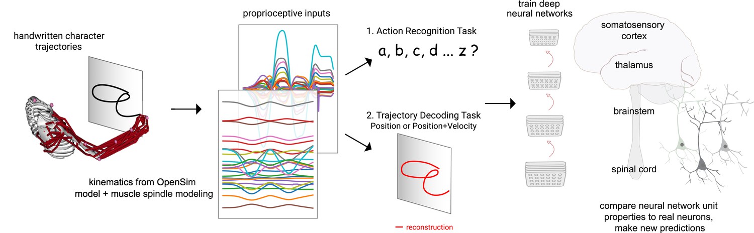
Contrasting spindle-based tasks to study proprioception: proprioceptive inputs that correspond to the tracing of individual letters were simulated using a musculoskeletal model of a human arm.
This scalable, large-scale dataset was used to train deep neural network models of the proprioceptive pathway either to classify the character (action recognition task [ART]) or to decode the posture of the arm (trajectory decoding tasks [TDTs]) based on the input muscle spindle firing rates. Here, we test two variants of the latter, to decode either position-only (canonical-proprioception) or position+velocity (as a control) of the end-effector. We then analyze these models and compare their tuning properties to the proprioceptive system of primates.
Figure 2 with 1 supplement
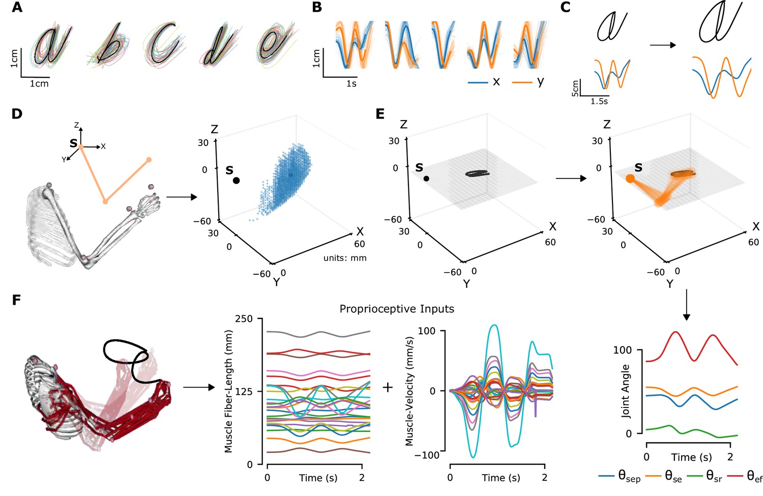
Synthetic proprioceptive characters dataset generation.
(A) Multiple examples of pen-tip trajectories for five of the 20 letters are shown. (B) The same trajectories as in A, plotted as time courses of Cartesian coordinates. (C) Creating (hand) end-effector trajectories from pen-tip trajectories. (Left) An example trajectory of character a resized to fit in a 10 × 10 cm2 grid, linearly interpolated from the true trajectory while maintaining the true velocity profile. (Right) This trajectory is further transformed by scaling, rotating, and varying its speed. (D) Candidate starting points to write the character in space. (Left) A 2-link, 4 degrees of freedom (DoFs) model human arm is used to randomly select several candidate starting points in the workspace of the arm (right), such that written characters are all strictly reachable by the arm. (E) (Left to right and down) Given a sample trajectory in (C) and a starting point in the arm’s workspace, the trajectory is then drawn on either a vertical or horizontal plane that passes through the starting point. We then apply inverse kinematics to solve for the joint angles required to produce the traced trajectory. (F) (Left to right) The joint angles obtained in (E) are used to drive a musculoskeletal model of the human arm in OpenSim, to obtain equilibrium muscle fiber-length trajectories of 25 relevant upper arm muscles. These muscle fiber lengths and their instantaneous velocities together form the proprioceptive inputs.
Figure 2—video 1
Supplementary video.
Video depicts the OpenSim model being passively moved to match the human-drawn character ‘a’ for three different variants; drawn vertically (left, right) and horizontally (middle).
Figure 3 with 1 supplement
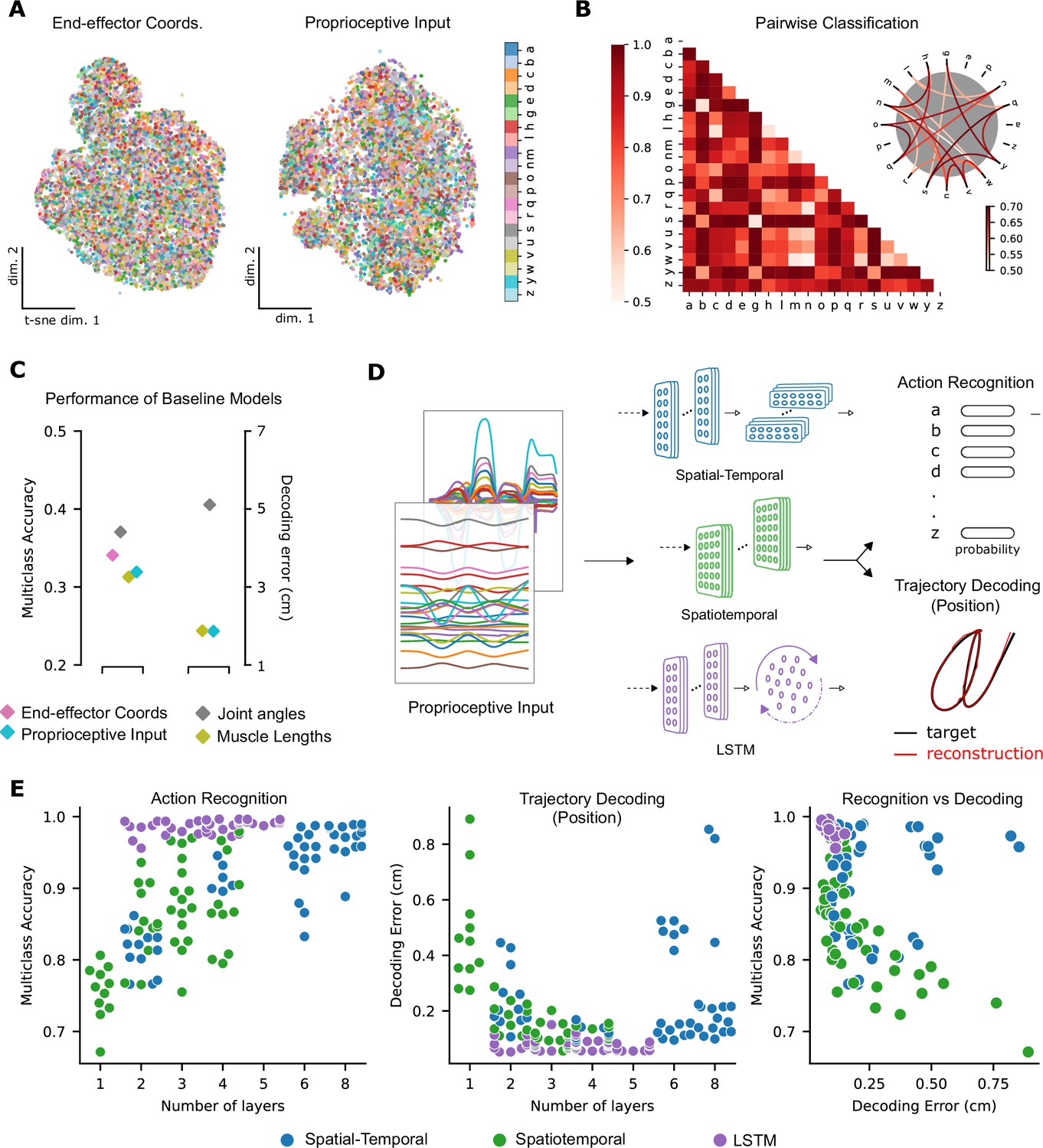
Quantifying action recognition and trajectory decoding task performance.
(A) t-Distributed stochastic neighbor embedding (t-SNE) of the end-effector coordinates (left) and proprioceptive inputs (right). (B) Classification performance for all pairs of characters with binary support vector machines (SVMs) trained on proprioceptive inputs. Chance level accuracy is 50%. The pairwise accuracy is 86.6 ± 12.5% (mean ± SD, pairs). A subset of the data is also illustrated as a circular graph, whose edge color denotes the classification accuracy. For clarity, only pairs with performance less than 70% are shown, which corresponds to the bottom 12% of all pairs. (C) Performance of baseline models: Multi-class SVM performance computed using a one-vs-one strategy for different types of input/kinematic representations on the action recognition task (left). Performance of ordinary least-squares linear regression on the trajectory decoding (position) task (right). Note that end-effector coordinates, for which this analysis is trivial, are excluded. (D) Neural networks are trained on two main tasks: action recognition and trajectory decoding (of position) based on proprioceptive inputs. We tested three families of neural network architectures. Each model is comprised of one or more processing layers, as shown. Processing of spatial and temporal information takes place through a series of one-dimensional (1D) or two-dimensional (2D) convolutional layers or a recurrent layer. (E) Performance of neural network models on the tasks: the test performance of the 50 networks of each type is plotted against the number of layers of processing in the networks for the action recognition (left) and trajectory decoding (center) tasks separately and against each other (right). Note we jittered the number of layers (x-values) for visibility, but per model it is discrete.
Figure 3—figure supplement 1
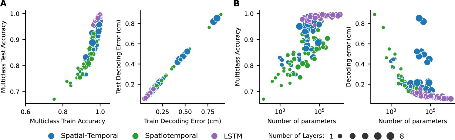
Network performance.
(A) Training vs. test performance for all networks. Shallower networks tend to overfit more. (B) Network performance is plotted against the number of parameters. Note: Parameters of the final (fully connected) layer are not counted.
Figure 4 with 1 supplement
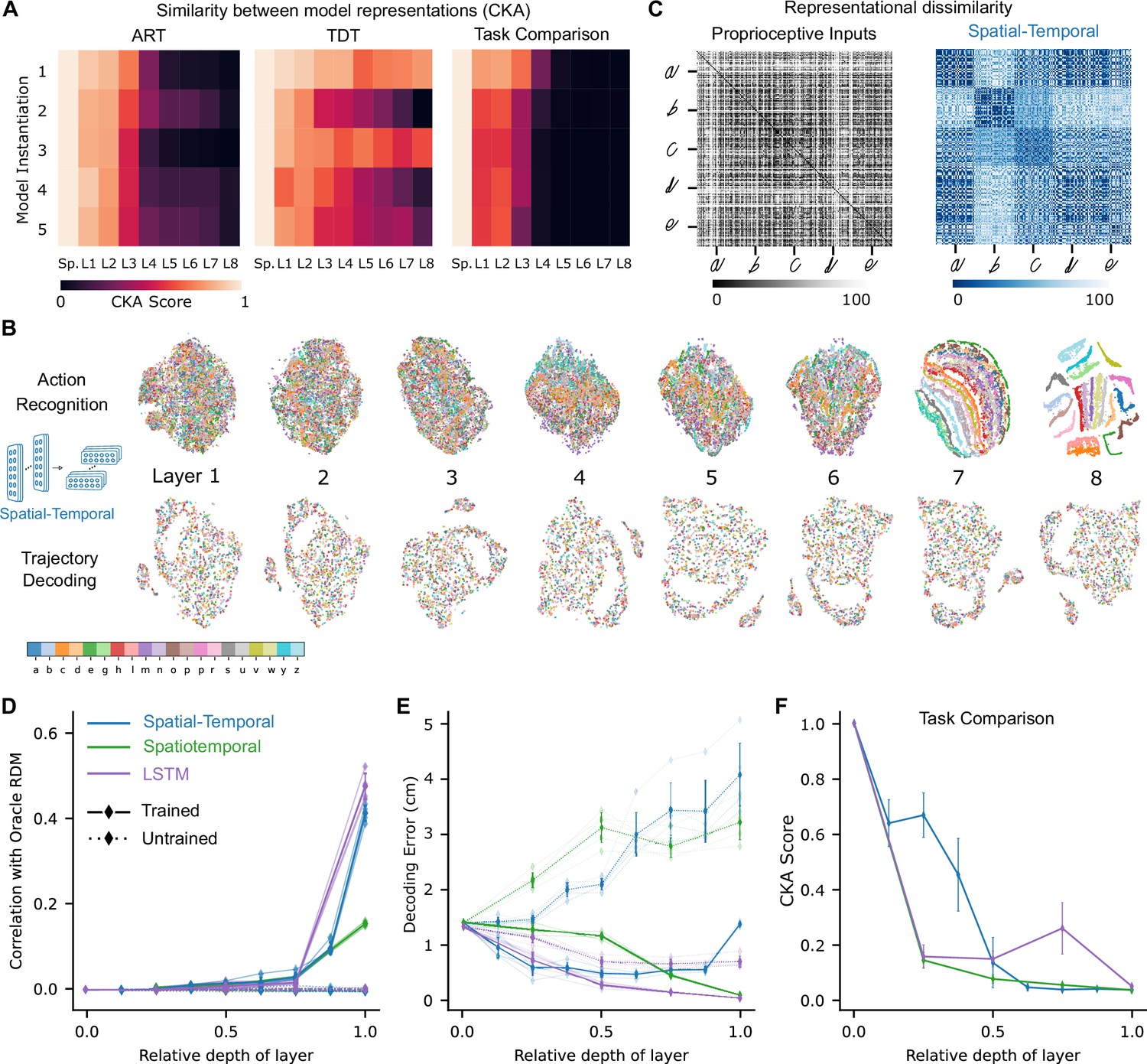
Low-dimensional embedding of network layers reveals structure.
(A) Similarity in representations (centered kernel alignment [CKA]) between the trained and the untrained models for each of the five instantiations of the best-performing spatial-temporal models (left and center). CKA between models trained on recognition vs. decoding (right). (B) t-Distributed stochastic neighbor embedding (t-SNE) for each layer of one instantiation of the best-performing spatial-temporal model trained on both tasks. Each data point is a random stimulus sample (N=2000, 50 per stimulus). (C) Representational dissimilarity matrices (RDMs). Character level representation is visualized using percentile RDMs for proprioceptive inputs (left) and final layer features (right) of one instantiation of the best-performing spatio-temporal model trained on the recognition task. (D) Similarity in stimulus representations between RDMs of an Oracle (ideal observer) and each layer for the five instantiations of the action recognition task (ART)-trained models and their untrained counterparts. (E) Decoding error (in cm) along the hierarchy for each model type on the trajectory decoding task. (F) Centered kernel alignment (CKA) between models trained on recognition vs. decoding for the five instantiations of all network types (right).
Figure 4—figure supplement 1
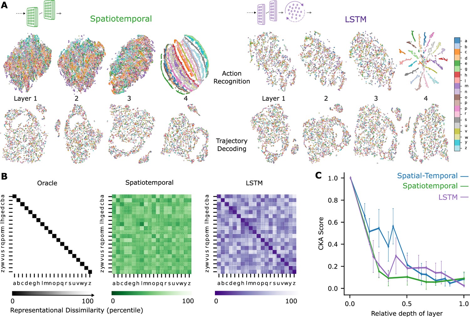
Extended analysis of network models.
(A) t-Distributed stochastic neighbor embedding (t-SNE) for each layer of the best spatiotemporal and long short-term memory (LSTM) model. Each data point is a random stimulus sample (N=4000, 200 per character). (B) Representational dissimilarity matrices (RDMs) of an ideal observer ‘Oracle’, which by definition has low dissimilarity for different samples of the same character and high dissimilarity for different samples of different characters. Character level representation are calculated through percentile RDMs for proprioceptive inputs and final layer features of one instantiation of the best-performing spatiotemporal and LSTM model trained on recognition task. (C) Centered kernel alignment (CKA) between models trained on recognition vs decoding for all network types ( per network type).
Figure 5 with 4 supplements
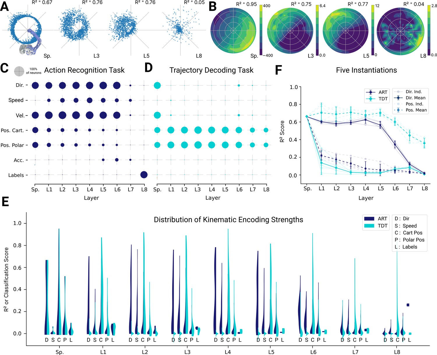
Analysis of single unit tuning properties for spatial-temporal models.
(A) Polar scatter plots showing the activation of units (radius ) as a function of end-effector direction, as represented by the angle θ for directionally tuned units in different layers of the top-performing spatial-temporal model trained on the action recognition task, where direction corresponds to that of the end-effector while tracing characters in the model workspace. The activation strengths of one (velocity-dependent) muscle spindle one unit each in layers 3, 5, and 8 are shown. (B) Similar to (A), except that now radius describes velocity and color represents activation strength. The contours are determined following linear interpolation, with gaps filled in by neighbor interpolation and smoothed using a Gaussian filter. Examples of one muscle spindle, one unit each in layers 3, 5, and 8, are shown. (C) For each layer of one trained instantiation, the units are classified into types based on their tuning. A unit was classified as belonging to a particular type if its tuning had a test . Tested features were direction tuning, speed tuning, velocity tuning, Cartesian and polar position tuning, acceleration tuning, and label tuning (18/5446 scores excluded for action recognition task [ART]-trained, 430/5446 for trajectory decoding task [TDT]-trained; see Methods). (D) The same plot but for the spatial-temporal model of the same architecture but trained on the trajectory decoding task. (E) For an example instantiation, the distribution of test scores for both the ART- and TDT-trained models are shown as vertical histograms (split-violins), for five kinds of kinematic tuning for each layer: direction tuning, speed tuning, Cartesian position tuning, polar position tuning, and label specificity indicated by different shades and arranged left-right for each layer including spindles. Tuning scores were excluded if they were equal to 1, indicating a constant neuron, or less than −0.1, indicating an improper fit (12/3890 scores excluded for ART, 285/3890 for TDT; see Methods). (F) The means of 90% quantiles over all five model instantiations of models trained on ART and TDT are shown for direction tuning (dark) and position tuning (light). 95% confidence intervals are shown over instantiations ().
Figure 5—figure supplement 1
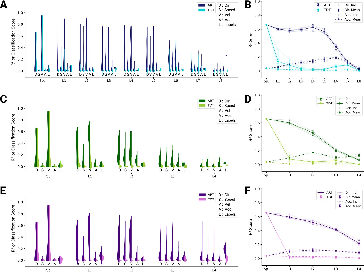
Extended kinematic tuning of single neurons.
(A) For an example spatial-temporal model instantiation, the distribution of test scores for both the action recognition task (ART)- and trajectory decoding task (TDT)-trained models are shown, for direction, speed, velocity, acceleration, and labels (12/3890 scores excluded over all layers for ART-trained, 290/3890 for TDT-trained; see Methods). (B) The individual traces (faint) as well as the means (dark) of 90% quantiles over all five model instantiations of models trained on action recognition and trajectory decoding are shown for direction tuning (solid line) and acceleration tuning (dashed line). (C, D) Same as (A, B) but for the spatiotemporal model (0/2330 scores excluded for ART-trained, 138/2330 for TDT; see Methods). (E, F) Same as (A, B) but for the long short-term memory (LSTM) model (10/6530 scores excluded for ART-trained, 1052/6530 for TDT-trained; see Methods).
Figure 5—figure supplement 2
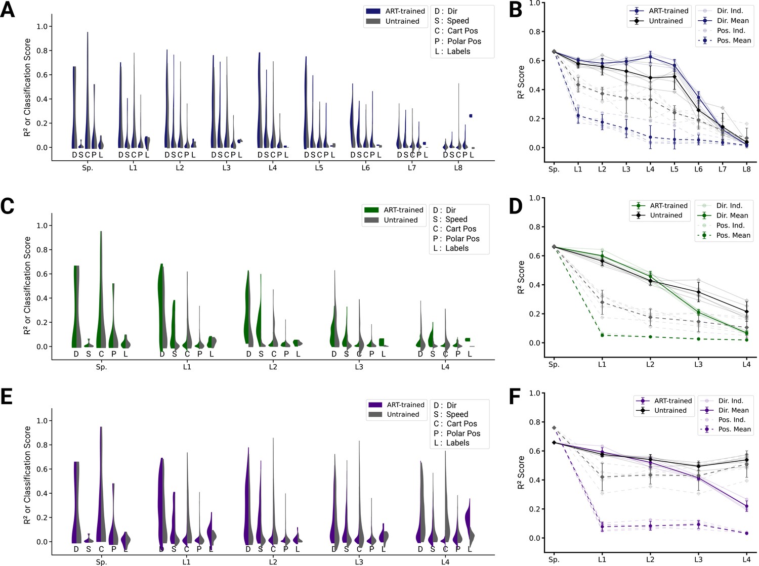
Analysis of single unit tuning properties for action recognition task (ART)-trained and untrained models.
(A) For an example instantiation of the top-performing spatial-temporal model, the distribution of test scores for both the trained and untrained model are shown, for five kinds of kinematic tuning for each layer: direction tuning, speed tuning, Cartesian position tuning, polar position tuning, and label specificity. The solid line connects the 90% quantiles of two of the tuning curve types, direction tuning (dark) and position tuning (light) (12/3890 scores excluded summed over all layers for ART-trained, 351/3890 for untrained; see Methods). (B) The means of 90% quantiles over all five model instantiations of models trained on action recognition and trajectory decoding are shown for direction tuning (dark) and position tuning (light). 95% confidence intervals are shown over instantiations (). (C) The same plot as in (A) but for the top-performing spatiotemporal model (0/2330 scores excluded for ART-trained, 60/2330 for the untrained; see Methods). (D) The same plot as (B) for the spatiotemporal model. (E) The same plot as in (A) but for the top-performing long short-term memory (LSTM) model (10/6530 scores excluded for ART-trained, 395/6530 for the untrained; see Methods). (F) The same plot as (B) for the LSTM model.
Figure 5—figure supplement 3
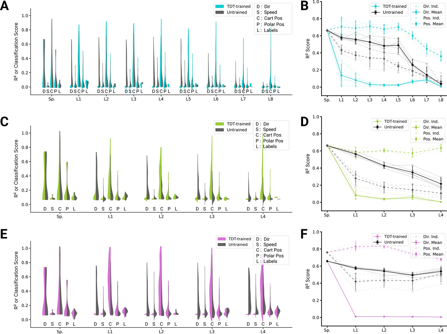
Analysis of single unit tuning properties for trajectory decoding task (TDT)-trained and untrained models.
(A) For an example instantiation of the top-performing spatial-temporal model, the distribution of test scores for both the trained and untrained model are shown, for five kinds of kinematic tuning for each layer: direction tuning, speed tuning, Cartesian position tuning, polar position tuning, and label specificity. The solid line connects the 90% quantiles of two of the tuning curve types, direction tuning (dark) and position tuning (light) (285/3890 scores excluded summed over all layers for TDT-trained, 351/3890 for untrained; see Methods). (B) The means of 90% quantiles over all five model instantiations of models trained on action recognition and trajectory decoding are shown for direction tuning (dark) and position tuning (light). 95% confidence intervals are shown over instantiations (). (C) The same plot as in (A) but for the top-performing spatiotemporal model (138/2330 scores excluded for TDT-trained, 60/2330 for the untrained; see Methods). (D) The same plot as (B), for the spatiotemporal model. (E) The same plot as in (A) but for the top-performing long short-term memory (LSTM) model (1052/6530 scores excluded for TDT-trained, 395/6530 for the untrained; see Methods). (F) The same plot as (B), for the LSTM model.
Figure 5—figure supplement 4
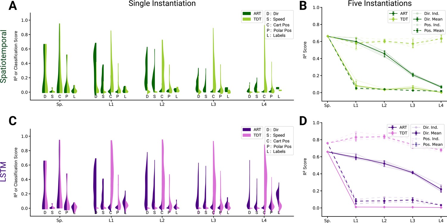
Analysis of single unit tuning properties for spatiotemporal and long short-term memory (LSTM) models.
(A) For an example instantiation of the top-performing spatiotemporal model, the distribution of test scores for both the action recognition task (ART)-trained and trajectory decoding task (TDT)-trained model are shown, for five kinds of kinematic tuning for each layer: direction tuning, speed tuning, Cartesian position tuning, polar position tuning, and label specificity. The solid line connects the 90% quantiles of two of the tuning curve types, direction tuning (dark) and position tuning (light) (0/2330 scores excluded summed over all layers for ART-trained, 138/2330 for TDT; see Methods). (B) The means of 90% quantiles over all five model instantiations of models trained on action recognition and trajectory decoding are shown for direction tuning (dark) and position tuning (light). 95% confidence intervals are shown over instantiations (). (C) The same plot as in (A) but for the top-performing LSTM model (10/6530 scores excluded for ART-trained, 1052/6530 for TDT; see Methods). (D) The same plot as (B), for the LSTM model.
Figure 6 with 3 supplements
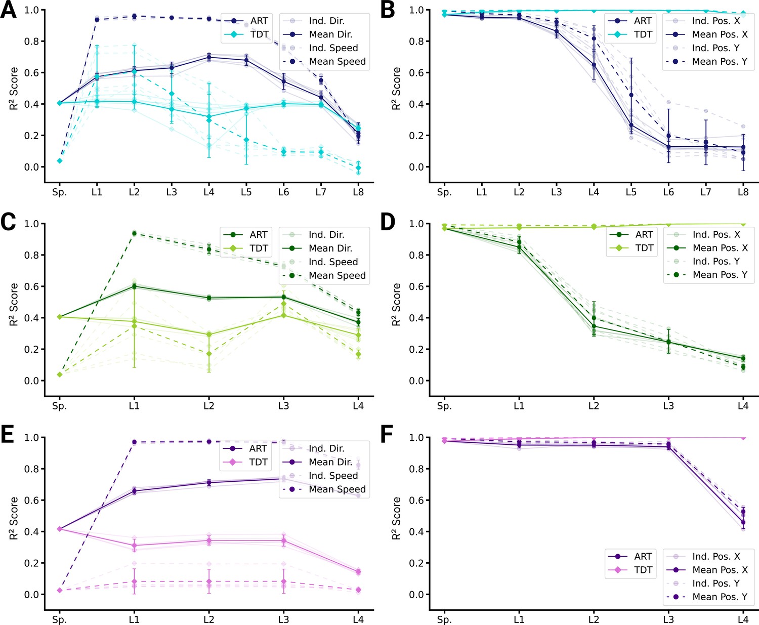
Population decoding analysis of action recognition task (ART) vs. trajectory decoding task (TDT) models.
(A) Population decoding of speed (light) and direction (dark) for spatial-temporal models for the ART- and TDT-trained models. The faint line shows the score for an individual model; the dark one the mean over all instantiations (). (B) Population decoding of end-effector position (X and Y coordinates) for spatial-temporal models. The faint line shows the score for an individual model; the dark one the mean over all instantiations (). (C) Same as (A) but for spatiotemporal models. (D) Same as (B) but for spatiotemporal models. (E) Same as (A) but for long short-term memory (LSTM) models. (F) Same as (B) but for LSTM models.
Figure 6—figure supplement 1
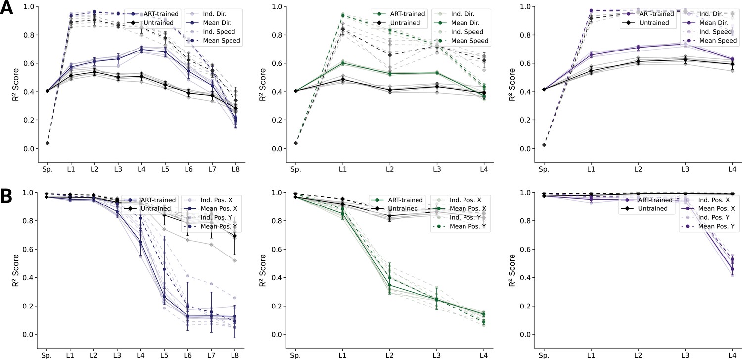
Analysis of population decoding for action recognition task (ART)-trained and untrained models.
(A) Population decoding of speed (light) and direction (dark) for the ART-trained and untrained for spatial-temporal models (left), spatiotemporal (middle), and long short-term memory (LSTM) (right) models. The faint line shows the score for an individual model; the dark one the mean over all instantiations (). (B) Population decoding of end-effector position (X and Y coordinates) for spatial-temporal models. The faint line shows the score for an individual model; the dark one the mean over all instantiations ().
Figure 6—figure supplement 2
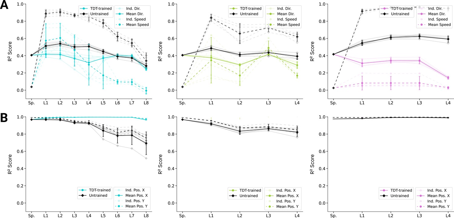
Analysis of population decoding for trajectory decoding task (TDT)-trained and untrained models.
(A) Population decoding of speed (light) and direction (dark) for the TDT-trained and untrained for spatial-temporal models (left), spatiotemporal (middle), and long short-term memory (LSTM) (right) models. The faint line shows the score for an individual model; the dark one the mean over all instantiations (). (B) Population decoding of end-effector position (X and Y coordinates) for spatial-temporal models (left), spatiotemporal (middle), and LSTM (right) models. The faint line shows the score for an individual model; the dark one the mean over all instantiations ().
Figure 6—figure supplement 3
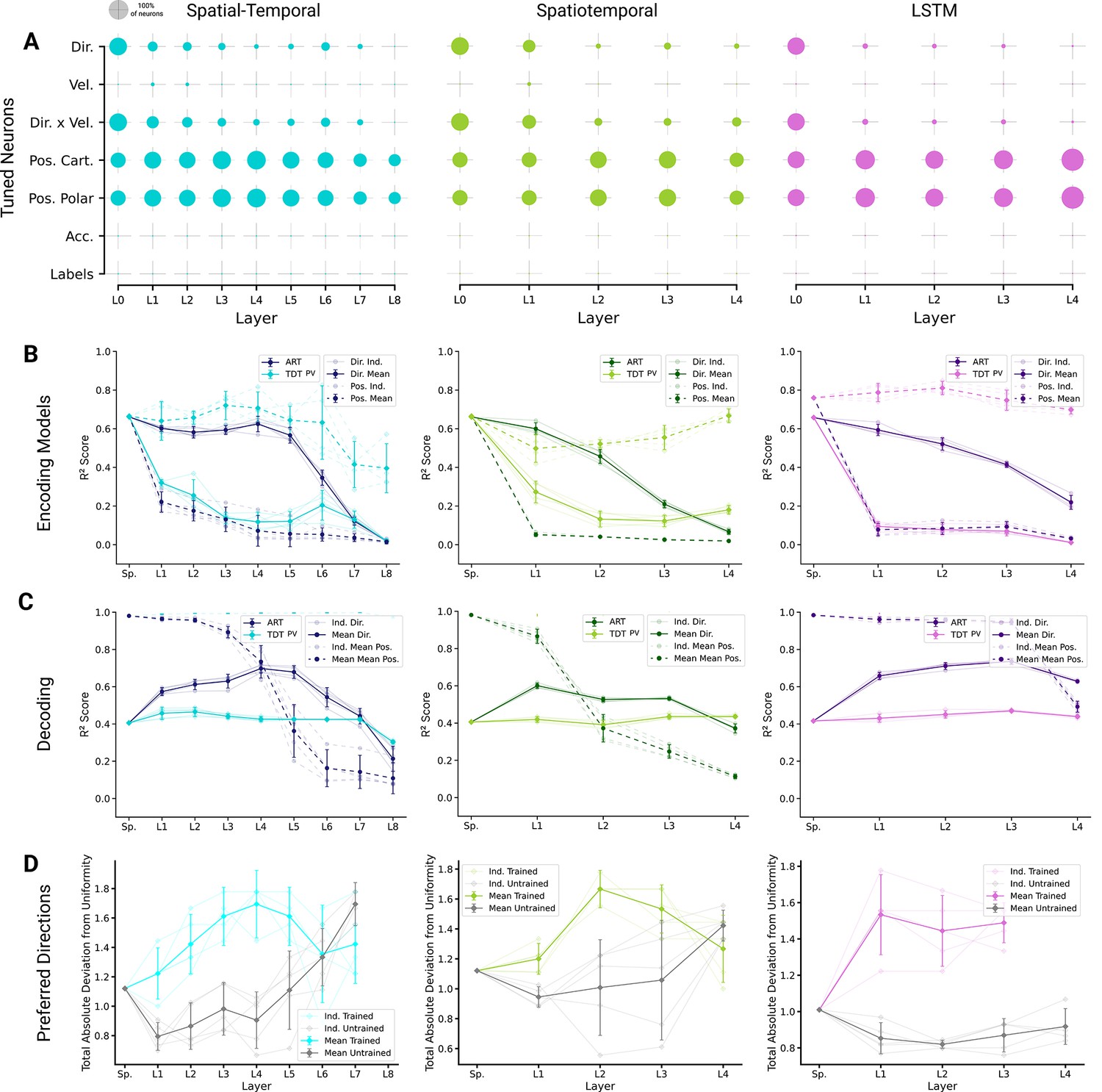
Results for the position and velocity trajectory decoding task (TDT-PV).
(A) For an example instantiation, the fraction of neurons that are tuned for a particular feature ( on the relevant encoding model). Model architectures: (left) spatial-temporal, (middle) spatiotemporal, (right) long short-term memory (LSTM). Tested features were direction tuning, speed tuning, velocity tuning, Cartesian and polar position tuning, acceleration tuning, and label tuning (328/5446 scores excluded for TDT-PV-trained spatial-temporal model, 140/3262 for spatiotemporal, and 1150/9142 for LSTM; see Methods). (B) The means of 90% quantiles over all five model instantiations of models trained on action recognition task (ART) and TDT-PV are shown for direction tuning (dark) and position tuning (light). 95% confidence intervals are shown over instantiations (). (C) Population decoding of direction (dashed) and Cartesian coordinates (solid; mean over individually computed scores for X and Y directions taken) for the ART-trained and TDT-PV-trained for spatial-temporal models (left), spatiotemporal (middle), and LSTM (right) models. The faint line shows the score for an individual model; the dark one the mean over all instantiations (). (D) For quantifying uniformity, we calculated the total absolute deviation from the corresponding uniform distribution over the bins in the histogram (red line in inset) for the spatial-temporal model (left), the spatiotemporal model (middle), and the LSTM model (right). Normalized absolute deviation from uniform distribution for preferred directions per instantiation is shown (, faint lines) for TDT-PV-trained and untrained models as well as mean and 95% confidence intervals over instantiations (solid line; ).
Figure 7 with 1 supplement
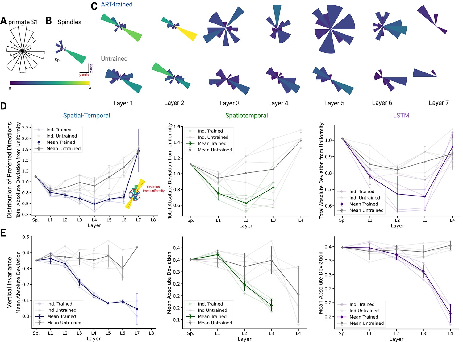
Distribution of preferred directions and invariance of representation across workspaces.
(A) Adopted from Prud’homme and Kalaska, 1994; distribution of preferred directions in primate S1. (B) Distribution of preferred directions for spindle input. (C) Distribution of preferred directions for one spatial-temporal model instantiation (all units with are included). Bottom: the corresponding untrained model. For visibility, all histograms are scaled to the same size and the colors indicate the number of tuned neurons. (D) For quantifying uniformity, we calculated the total absolute deviation from the corresponding uniform distribution over the bins in the histogram (red line in inset) for the spatial-temporal model (left), the spatiotemporal model (middle), and the long short-term memory (LSTM) model (right). Normalized absolute deviation from uniform distribution for preferred directions per instantiation is shown (, faint lines) for trained and untrained models as well as mean and 95% confidence intervals over instantiations (solid line; ). Note that there is no data for layers 7 and 8 of the trained spatial-temporal model, layer 8 of the untrained spatial-temporal model, and layer 4 of the spatiotemporal model as they have no direction-selective units (). (E) For quantifying invariance, we calculated mean absolute deviation in preferred orientation for units from the central plane to each other vertical plane (for units with ). Results are shown for each instantiation (, faint lines) for trained and untrained models plus mean (solid) and 95% confidence intervals over instantiations (). Note that there is no data for layer 4 of the trained spatiotemporal model, as it has no direction-selective units ().
Figure 7—figure supplement 1
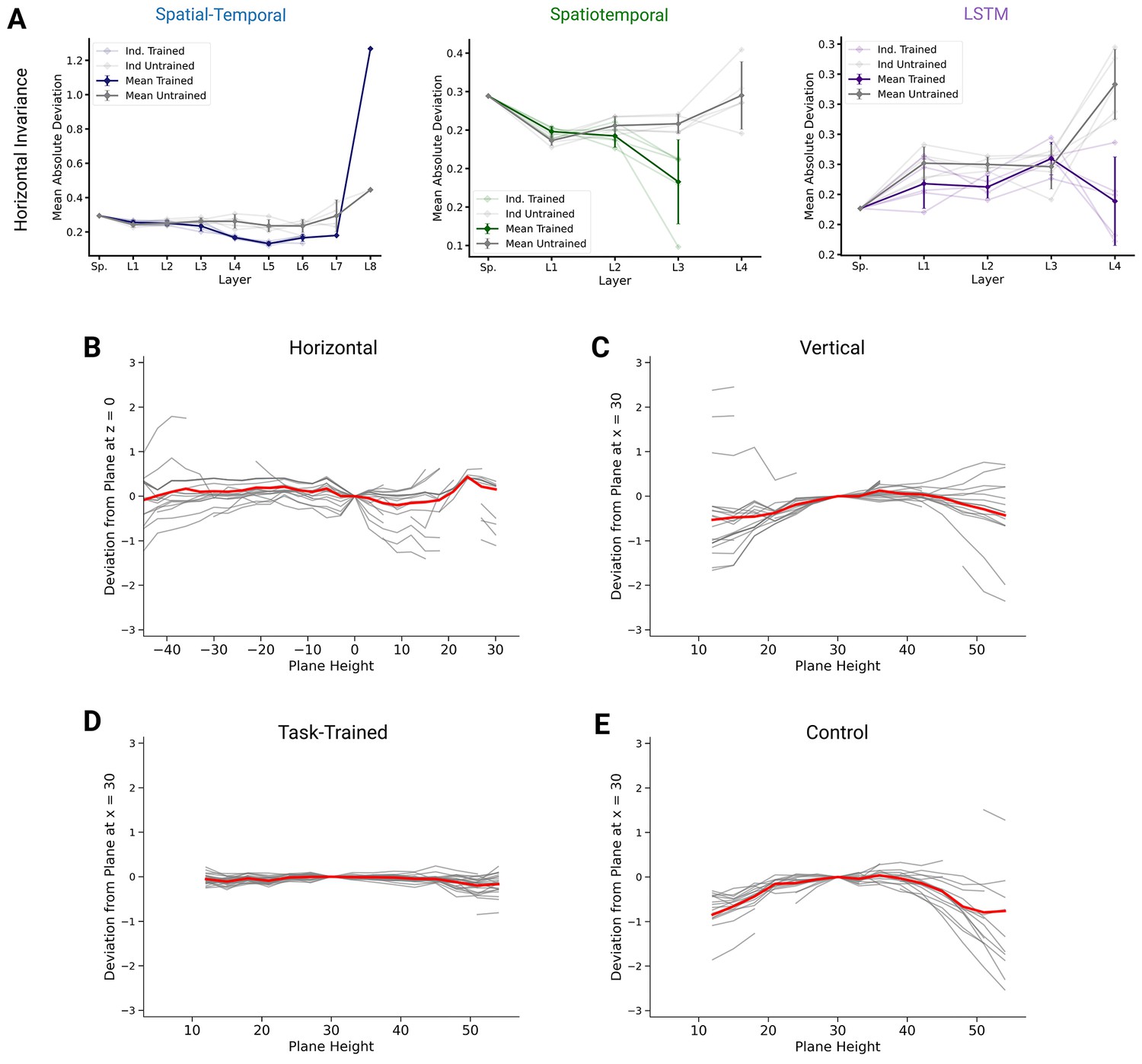
Invariance of preferred orientations.
(A) To quantify invariance, we calculated mean absolute deviation in preferred orientation for units from a central plane at to each other horizontal plane (for units with ). Results are shown for each instantiation (, faint lines) for trained and untrained models plus mean (solid) and 95% confidence intervals over instantiations () for the spatial-temporal (left), spatiotemporal (right), and long short-term memory (LSTM) (right) networks. Note that there is no data for layer 4 of the trained spatiotemporal model, as it has no direction-selective units (). (B) Deviation in preferred direction for individual spindles (N=25). The preferred directions are fit for each plane and displayed in relation to a central horizontal (left) and vertical plane (right). Individual gray lines are for all units (spindles) with , the thick red line marks the mean. (C) Same as (B), but for direction tuning in vertical planes for units in layer 5 of one instantiation of the best spatial-temporal model for the trained (left) and untrained model (right). Individual gray lines are for units with , and the red line is the plane-wise mean. (D) Same as in (B) but for layer 5 of the trained spatial-temporal network. (E) Same as in (D) but for layer 5 of the corresponding untrained network.
Tables
Table 1
Variable range for the data augmentation applied to the original pen-tip trajectory dataset.
Furthermore, the character trajectories are translated to start at various starting points throughout the arm’s workspace, overall yielding movements in 26 horizontal and 18 vertical planes.
| Type of variation | Levels of variation |
|---|---|
| Scaling | [0.7×, 1×, 1.3×] |
| Rotation | [-π/6, -π/12, 0, π/12, π/6] |
| Shearing | [-π/6, -π/12, 0, π/12, π/6] |
| Translation | Grid with a spacing of 3 cm |
| Speed | [0.8×, 1×, 1.2×, 1.4×] |
| Plane of writing | [Horizontal (26), Vertical (18)] |
Table 2
Hyper-parameters for neural network architecture search.
To form candidate networks, first a number of layers (per type) is chosen, ranging from 2 to 8 (in multiples of 2) for spatial-temporal models and 1–4 for the spatiotemporal and long short-term memory (LSTM) ones. Next, a spatial and temporal kernel size per Layer is picked where relevant, which remains unchanged throughout the network. For the spatiotemporal model, the kernel size is equal in both the spatial and temporal directions in each layer. Then, for each layer, an associated number of kernels/feature maps is chosen such that it never decreases along the hierarchy. Finally, a spatial and temporal stride is chosen. For the LSTM networks, the number of recurrent units is also chosen. All parameters are randomized independently and 50 models are sampled per network type. Columns 2–4: Hyper-parameter values for the top-performing models in the ART. The values given under the spatial rows count for both the spatial and temporal directions for the spatiotemporal model.
| Hyper-parameters | Spatial-temporal | Spatiotemporal | LSTM | |
|---|---|---|---|---|
| Num. layers | [1, 2, 3, 4] | 4+4 | 4 | 3+1 |
| Spatial kernels (pL) | [8, 16, 32, 64] | [8,16,16,32] | [8, 8, 32, 64] | [8, 16, 16] |
| Temporal kernels (pL) | [8, 16, 32, 64] | [32, 32, 64, 64] | n/a | n/a |
| Spatial kernel size | [3, 5, 7, 9] | 7 | 7 | 3 |
| Temporal kernel size | [3, 5, 7, 9] | 2 | n/a | n/a |
| Spatial stride | [1, 2] | 9 | 2 | 1 |
| Temporal stride | [1, 2, 3] | 3 | n/a | n/a |
| Num. recurrent units | [128, 256] | n/a | n/a | 256 |
Table 3
Size of representation at each layer for best-performing architecture of each network type (spatial × temporal × filter dimensions).
| Layer | Dimension | Layer | Dimension | Layer | Dimension |
|---|---|---|---|---|---|
| Input | 25 × 320 × 2 | Input | 25 × 320 × 2 | Input | 25 × 320 × 2 |
| SC0 | 13 × 320 × 8 | STC0 | 13 × 160 × 8 | SC0 | 25 × 320 × 8 |
| SC1 | 7 × 320 × 16 | STC1 | 7 × 80 × 8 | SC1 | 25 × 320 × 16 |
| SC2 | 4 × 320 × 16 | STC2 | 4 × 40 × 32 | SC2 | 25 × 320 × 16 |
| SC3 | 2 × 320 × 32 | STC3 | 2 × 20 × 64 | R | 256 × 320 |
| TC0 | 2 × 107 × 32 | ||||
| TC1 | 2 × 36 × 32 | ||||
| TC2 | 2 × 12 × 64 | ||||
| TC3 | 2 × 4 × 64 |
Additional files
Download links
A two-part list of links to download the article, or parts of the article, in various formats.
Downloads (link to download the article as PDF)
Open citations (links to open the citations from this article in various online reference manager services)
Cite this article (links to download the citations from this article in formats compatible with various reference manager tools)
Contrasting action and posture coding with hierarchical deep neural network models of proprioception
eLife 12:e81499.
https://doi.org/10.7554/eLife.81499


