Spatial structure favors microbial coexistence except when slower mediator diffusion weakens interactions

Version of Record

Accepted for publication after peer review and revision.

Download
Cite
Share
CommentOpen annotations (there are currently 0 annotations on this page).

500 views

Version of Record published: July 14, 2023 (This version)
Accepted Manuscript published: June 23, 2023 (Go to version)
Accepted: June 20, 2023
Received: August 6, 2022
Preprint posted: August 1, 2022 (Go to version)

1. Of interest
Gut Health: The value of connections

Vanessa Rossetto Marcelino

Insight Sep 19, 2023
Further reading

Abstract
Editor's evaluation
Introduction
Results
Discussion
Methods
Data availability
References
Decision letter
Author response
Article and author information
Metrics

Abstract

Microbes often exist in spatially structured environments and many of their interactions are mediated through diffusible metabolites. How does such a context affect microbial coexistence? To address this question, we use a model in which the spatial distributions of species and diffusible interaction mediators are explicitly included. We simulate the enrichment process, examining how microbial species spatially reorganize and how eventually a subset of them coexist. In our model, we find that slower motility of cells promotes coexistence by allowing species to co-localize with their facilitators and avoid their inhibitors. We additionally find that a spatially structured environment is more influential when species mostly facilitate each other, rather than when they are mostly competing. More coexistence is observed when species produce many mediators and consume some (not many or few) mediators, and when overall consumption and production rates are balanced. Interestingly, coexistence appears to be disfavored when mediators are diffusing slowly because that leads to weaker interaction strengths. Overall, our results offer new insights into how production, consumption, motility, and diffusion intersect to determine microbial coexistence in a spatially structured environment.

Editor's evaluation

This important study uses computational simulations to explore when spatial structure can promote the coexistence between different microbial species and when not, ultimately helping to explain diversity in microbial communities. The evidence supporting the conclusions is convincing, based on extensive parameter sweeps. The conclusion that spatial structure only promotes coexistence under certain conditions is a testable hypothesis that is very interesting to microbial ecologists quite broadly.

https://doi.org/10.7554/eLife.82504.sa0

Introduction

Microbes are rarely found in isolation in nature. Instead, they are found coexisting with one another in complex networks of interactions (Ma et al., 2020). Given the differences among taxa and the competitive forces that act between them, a fundamental question in microbial community ecology is how this coexistence is maintained (Chesson, 2000b; Solé and Bascompte, 2006; Widder et al., 2016). And because many important industrial, environmental, and health-related processes rely on microbial communities to function (e.g. anaerobic granules, microbial mats, and gut microbiota, respectively), understanding the conditions that favor microbial coexistence is critical to sustaining these systems.

Spatial structure and organization may shape coexistence via numerous mechanisms (Tilman, 1994; Durrett and Levin, 1994; Tilman and Kareiva, 1998; Durrett and Levin, 1998; Kerr et al., 2002; Brockhurst et al., 2006; Amarasekare, 2003), often by modulating the interactions among individuals. For example, in a spatially structured environment where progeny is more likely to be in the vicinity of parents, intensified intrapopulation competition can give less competitive species a chance to survive (Chesson, 2000a). In other conditions, spatial isolation can allow organisms with conflicting abiotic needs to flourish in appropriate environments (Kim et al., 2011; Satoh et al., 2007). The interplay between dispersal and competition can also allow coexistence between species that are more competitive growers and species that are better at dispersing and colonizing (Tilman, 1990).

Spatial heterogeneity has been invoked as a mechanism for microbial coexistence since the pioneering work by Gause, 1934. And although general concepts of coexistence are expected to apply equally to microbes, microbial communities may be affected by spatial structure in unique ways because of the scale and multiplicity of microbial interactions. An important and ubiquitous example of this are microbial interactions that are mediated via diffusible metabolites—including resources and metabolic byproducts. Spatial structure can stabilize these interactions and support coexistence, for example, by allowing cheaters to be excluded from beneficial interactions (Momeni et al., 2013b; Pande et al., 2016), or by permitting facilitative chemical interactions while preventing the inhibitory effects of an interacting organism’s physical presence (Kim et al., 2008). And while it is clear that the outcomes of interactions via diffusible mediators in structured environments may depend on mediator diffusion rates (Kümmerli et al., 2014; Allison, 2005) and the larger network of antagonistic and cooperative interactions (Nadell et al., 2016), how such factors translate into community-level consequences is not well understood.

Prior reports that address coexistence of metabolically interacting microbes in a spatially structured environment are scarce. In an implicit model, Murrell and Law, 2003 have shown in a modified Lotka–Volterra model that when interspecific competition operates over shorter distances than intraspecific competition a spatially structured environment can lead to species coexistence by allowing for aggregation. And in recent work with explicit modeling of space, Weiner et al., 2019 examined coexistence in territorial populations interacting through diffusible mediators and found that metabolic tradeoffs allow for the coexistence of more species than the number of nutrients.

Our model is distinct from previous work in that we allow overlap and dispersal of populations through the shared space. Our motivation is to capture situations in which microbes can disperse inside a matrix that defines the spatial structure. An example of this is the mucosal layer of the digestive or respiratory tract, in which stratification is possible, yet the distribution of different species populations can overlap. Another example is in yogurt or cheese, where spatial structure exists, but populations are not territorial. We modify a previously developed mediator-explicit model (Niehaus et al., 2019) to account for spatial structure and the dispersion of species in the same space. Here, we limit our study to one-dimensional (1D) spatial structure as a starting point. We examine in our model conditions under which coexistence is favored. We should emphasize that even though we choose our parameters within the range of typical values observed among microbial communities, the purpose of this work is not to recapture a specific community. Instead, by examining a range of values for parameters such as metabolite diffusion and species dispersal, we hope to gain a better understanding of how rates of these processes can affect species coexistence.

Results

A spatial mediator-explicit model of microbial communities

In our mediator-explicit model, species interact through metabolites that they produce and/or consume (Figure 1A, B; Niehaus et al., 2019). Each species can produce a subset of metabolites and consume a subset of metabolites. Each of the metabolites in the shared environment can in turn influence any of the species by increasing or decreasing their growth rate (i.e. facilitation or inhibition, respectively) compared to how each species grows in the absence of interactions (Niehaus et al., 2019). We also assume that different interaction mediators additively influence the overall growth rate of each species (see Model description in Methods).

Figure 1 with 9 supplements see all

Download asset Open asset

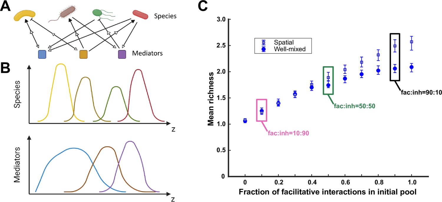
A spatial environment favors coexistence more when interspecies facilitation is prevalent in the initial species pool.

(A) Species are engaged in metabolite-mediated interactions with other species. Each species produces a subset of mediators and consumes a subset. Each mediator can positively or negatively modulate the growth rate of the species it influences. In our model, consumption is present whenever there is an influence from a mediator on a species, regardless of whether the influence is facilitative or inhibitory. Production and consumption of mediators are indicated by open arrows. (B) In a one-dimensional (1D) spatial context, species and mediators are defined as functions of space that change over time because of population growth and dispersal as well as mediator production, consumption, and diffusion. A cartoon representation of the distributions of four species and three mediators are shown here over the spatial context (z). (C) Simulations were run at different ratios of facilitative to inhibitory interactions (fac:inh) for spatial (open blue squares) and well-mixed (filled blue circles) communities. Each ratio was run 500 times with the richness (number of species stably surviving at the end of a simulation) averaged over all the simulations. Each simulation started with 10 species and 5 mediators and ran for 100 generations. The error bars are 95% confidence intervals generated by bootstrapping 100 samples. Here, the species dispersal coefficient is $5 \times 10^{- 9}$ cm²/hr. Boxes mark fac:inh ratios used in later simulations.

We assume a 1D spatial structure which preserves the spatial context but allows the diffusion of metabolites and dispersal of species. Multiple metabolites and species can be present in a single location. Both metabolite diffusion and species dispersal are modeled as random walk processes, characterized with a diffusion coefficient and a dispersal coefficient, respectively. In a typical simulation, we start from an initial distribution in which populations occupy adjacent, non-overlapping spatial locations at low initial density. This choice is made to impose a reproducible initial condition that emphasizes the role of space. Each simulation starts with a network of interactions in which interaction strengths, production and consumption links, and production and consumption rates are assigned randomly. The initial pool typically contains 10 species and 5 interaction mediators. We simulate community enrichment through rounds of growth and dilution (Niehaus et al., 2019; Goldford et al., 2018) for 100 generations, and assess the richness of each resulting community (i.e., the number of species stably persisting in the community). We have chosen 100 generations of growth, because we have observed that often this is enough to reliably decide which species stably persist in the community (Figure 1—figure supplement 1). At each dilution step, we assume that the overall spatial distribution of the community is preserved and all populations at all locations are diluted with the same factor. We recognize that this assumption is not universally true; however, we adopt it as an approximation, in the absence of additional information about a particular community. Such a dilution preserves some of the spatial structure of the community in the next round of growth and could represent a biofilm getting partially washed away by rain or in a microfluidic device, gut microbiota after a defecation event, or a broken-off portion of a granule initiating a new granule. We use a well-mixed version (Niehaus et al., 2019)—devoid of any spatial context—with the same set of parameters for species properties and interactions (i.e. consumption and production rates, basal growth rates, mediator influences, etc.) for all comparisons. Figure 1—figure supplement 2 shows an example of the population distributions and dynamics during the course of enrichment. In a simple example, we show that interactions and subsequently the population dynamics are affected by growing in a well-mixed versus spatial environment (Figure 1—figure supplement 3). We explored the impact of the overall spatial extent of the community and found that within an order of magnitude of change, the outcomes remained the same (Figure 1—figure supplement 4).

The shift from interspecies competition to intraspecies competition can favor coexistence in a spatially structured environment. To assess this impact, we imposed a cap on total cell number at each location in space. As this cap became more restrictive, it suppressed the most competitive species and led to higher coexistence (Figure 1—figure supplement 5). Since our focus in this manuscript is the impact of interspecies interactions, in the rest of this manuscript we pick the total cell number cap at a level (k_Y = 10⁹ cells/ml) that minimizes the impact of imposed intrapopulation competition.

A spatial environment favors coexistence more when facilitation among species is prevalent

We first examined how the prevalence of facilitative versus inhibitory interactions impacted coexistence in spatial communities. In our simulations, we dictated the ratio of facilitative and inhibitory interactions in the initial pool of species. Our results show that, similar to a well-mixed environment, more facilitative interactions lead to higher richness in communities that emerge from enrichment (Figure 1C, along the x-axis). Additionally, we observe that spatial communities show more coexistence than well-mixed communities when facilitation among species is prevalent (Figure 1C, spatial versus well-mixed). The same pattern, although less pronounced, was present when instead of richness we used the Shannon index to assess the diversity of resulting communities (Figure 1—figure supplement 2). Our explanation is that species locally grow better when adjacent to a facilitative partner and grow worse when in the vicinity of an inhibitory partner. The resulting spatial self-organization in effect amplifies facilitative interactions and dampens inhibitory interactions, leading to more coexistence. This is supported by our data which shows that the position of specific species with respect to other species that facilitate or inhibit it can impact the population dynamics (Figure 1—figure supplement 8). Because of the marked impact of the fac:inh ratio (i.e. the ratio of the number of facilitative interactions to the number of inhibitory interactions), moving forward, we will examine three conditions, with equal fractions of facilitative and inhibitory influences (fac:inh = 50:50), mostly inhibitory (fac:inh = 10:90), or mostly facilitative (fac:inh = 90:10) to scope the impact on coexistence.

At low species dispersal, self-organization is one of the mechanisms that can lead to a difference between spatial and well-mixed communities (Figure 1—figure supplement 3). In a simplified interpretation, self-organization can be in the form of co-localization driven by facilitation or segregation driven by inhibition. In our simulations, we observed that co-localization had a stronger effect on coexistence. The positive influence was reinforced by more growth in the vicinity of the partner, leading to a stronger representation of facilitation in spatial communities. In contrast, segregation only had a modest effect on weakening the impact of inhibition. As a result, there is more similarity between well-mixed and spatial communities in the absence of strong facilitative interactions (Figure 1C).

Coexistence is favored when many metabolites are produced and influence an intermediate number of species

Because metabolites are at the center of interspecies interactions in our model, we examined their impact on spatial coexistence of the average number of metabolites produced by each species and the average number of species influenced by each mediator. We found that coexistence is favored when the number of metabolites produced is larger (Figure 2, along the y-axis). This effect was stronger when the metabolite influences were mostly facilitative (fac:inh = 90:10, versus 50:50 or 10:90). In contrast, coexistence achieved its maximum values at intermediate ranges of mediator influence (Figure 2, x-axis), that is lower coexistence was observed when each mediator influenced too many or too few species on average. We note that these trends were largely the same between spatial and well-mixed communities.

Figure 2 with 4 supplements see all

Download asset Open asset

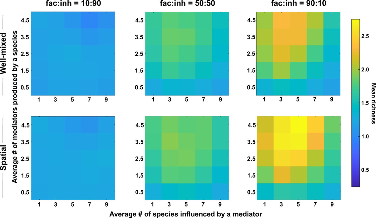
The number of metabolites produced and number of species influenced affect coexistence in spatial and well-mixed communities.

Different ranges of production and mediator influence values were analyzed for both well-mixed and spatial communities at three different fractions of fac:inh influences in the initial pool of species (10:90, 50:50, and 90:10). Mean richness (i.e. average number of species stably present at the end of a simulation) was calculated for 500 simulated instances and marked on the color bar. Each simulation started with 10 species and 5 mediators and ran for 100 generations. The x-axis represents the average number of species influenced by a mediator and the y-axis represents the average number of mediators produced by each species. Other simulation parameters are listed in Table 1.

Our explanation is that a larger range of production offers more opportunities for interaction, which through the enrichment process lead to the selection of facilitative subsets that coexist (Niehaus et al., 2019). A low mediator influence range works in the opposite direction, reduces opportunities for interactions and results in lower coexistence. Very high mediator influence range potentially leads to more self-facilitation (i.e. producing a metabolite that is beneficial to the producer species), which our data suggest can lead to take-over by a single species and a lower coexistence as a result (Figure 2—figure supplement 1).

Coexistence is higher when there is balance between production and consumption of mediators

We next asked how the rates of production and consumption of mediators would influence coexistence. To address this question, we surveyed a range of average rates of production and consumption. We observed that the highest levels of coexistence occurred when there was a balance between consumption and production rates among species, with slightly higher production than consumption (Figure 3).

Figure 3 with 3 supplements see all

Download asset Open asset

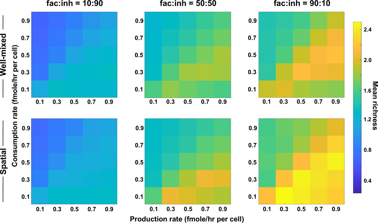
Coexistence is higher where there is a balance between production and consumption of mediators.

Different average production and consumption rates were analyzed for both well-mixed and spatial communities at three different fractions of fac:inh influences in the initial pool of species (10:90, 50:50, and 90:10). Mean richness (i.e. average number of species stably present at the end of a simulation) is calculated for 500 simulated instances. Each simulation started with 10 species and 5 mediators and ran for 100 generations. Color bar represents the average richness. The x-axis represents the average production rate of mediators and the y-axis represents the average consumption rate of mediators. Other simulation parameters are listed in Table 1.

Our justification for the observed pattern is that in one extreme where production is too high (lower right corner of each plot), mediators will build up in the environment. This will put the community in a regime in which consumption is not enough to create a feedback, that is ‘reusable mediators’ as discussed in Niehaus et al., 2019, which leads to lower coexistence. In the other extreme, when consumption is too high (upper left corner of each plot), metabolites that mediate the interactions will be depleted from the environment, leading to an effectively weaker interaction and thus lower coexistence. However, when production is slightly higher than consumption, metabolite quantities are sufficient to create strong interactions and facilitation feedbacks, leading to higher coexistence. While coexistence is slightly higher in the spatial communities compared to well-mixed ones, the production–consumption trends apply equally to spatial and well-mixed communities, as expected.

Limited species dispersal in a spatial environment allows more coexistence, especially when facilitation is common

Because species dispersal is a major factor in preserving community spatial structure, we examined how the dispersal coefficient affected coexistence outcomes. For this, we kept the diffusion coefficient of the mediators fixed and surveyed mean richness among many instances of communities randomly assembled (n = 500). When the diffusion coefficient for species approaches zero and cells remain in their original spatial location, we observe higher levels of coexistence (Figure 4). We also observed that the impact of lower dispersal is stronger in communities in which most interactions are facilitative rather than inhibitory. Our explanation is that lower dispersal rates mean that species grow best in spatial locations that are more supportive for their growth, which is in the vicinity of their beneficial partners and away from competitors or inhibitors. As discussed in Figure 1, such self-organization effectively amplifies facilitative interactions and de-emphasizes inhibitory interactions, leading to a higher coexistence. This is also consistent with the observation that the effect of dispersal rate is strongest when the proportion of facilitative interactions is highest. As the dispersal coefficient increases, the self-organization gets washed away by dispersal of cells to less than ideal locations for their growth and its benefit for coexistence diminishes.

Figure 4 with 4 supplements see all

Download asset Open asset

Lower dispersal rates allow more microbial coexistence.

Communities in spatially structured environments were simulated with different dispersal coefficients at three different fractions of fac:inh influences (10:90, 50:50, and 90:10). Mean richness (i.e. average number of species stably present at the end of a simulation) was calculated for 500 simulated instances. Each simulation started with 10 species and 5 mediators and ran for 100 generations. Other simulation parameters are listed in Table 1. The error bars are 95% confidence intervals generated by bootstrapping 100 samples.

At intermediate levels of dispersal, the trend reversed and well-mixed communities showed more coexistence compared to spatial communities. This is interesting because at the limit of extremely rapid diffusion (shown with a ‘∞’ sign in Figure 4) when we kept the species distribution uniform across the spatial extent, coexistence outcomes matched the well-mixed case, as expected. We found two factors that contributed to this trend. The first contribution came from longer-term changes in dynamics at intermediate levels of dispersal. Even after 100 generations, which is the typical extent of our studies, at intermediate levels of dispersal (e.g. D_Cell = 5 × 10⁻⁶ cm²/hr), the spatial distribution of populations is still changing considerably. As a result, our strict criteria for stable coexistence removes some of the populations that are still temporally not stable enough, leading to a lower overall assessment of coexistence in these cases. To show this, we examined the range of dispersal coefficients again, but kept all the species that were present after 100 generations, rather than those with stable population fractions at that point (see Model implementation in Methods). The results show that higher dispersal coefficients using this measure lowers the richness of resulting communities (based on presence, rather than stable presence), but not below the levels expected from well-mixed communities (Figure 4—figure supplement 1). As a second factor, we hypothesized that self-facilitation interactions contribute to the decrease in coexistence at intermediate dispersal levels. Our rationale was that self-facilitation interactions are amplified in communities in which the spatial context is preserved, because the distribution of producers matches the distribution of self, but not other recipients in such a case. This can lead to community overtake by a self-facilitating species. This effect will be weaker in communities at intermediate dispersal rates: at low dispersal rates self-facilitating species will be more confined in space and some of the metabolite will leak out to other species; in the other extreme, in the very high dispersal rates all distributions will become uniform and the distinction between self and others diminishes. To test this, we tested weaker self-facilitation links in our simulations and observed that this change led to higher coexistence in communities with intermediate dispersal coefficients but not in well-mixed communities or communities with low dispersal coefficients (Figure 4—figure supplement 2). It is a matter of debate how prevalent self-facilitation interactions are within microbial communities. Self-facilitation interactions do exist, for example when a species breaks down a recalcitrant substrate such as cellulose into smaller molecules that can be beneficial. However, if they are not as prevalent as what our model assumes, some of our predictions might be affected.

Coexistence is disrupted when the diffusion of mediators is too slow

The rate of diffusion of metabolites also has the potential to affect coexistence. We investigated coexistence over a range of mediator diffusion coefficients. We still typically observe a higher mean richness for spatial communities compared with the well-mixed communities (Figure 5). However, unlike the conventional wisdom, as the diffusion of mediators becomes slower, coexistence in spatial communities decreases. At low diffusion coefficients, coexistence drops even below that of corresponding well-mixed communities. We associate this trend to weaker effective interactions among species at lower diffusion coefficients. Mediators that are involved in facilitation play a major part in allowing coexistence of species (Niehaus et al., 2019); if these mediators get consumed by nearby species and do not travel long enough to reach other members of the community, the interaction-driven mechanism of coexistence is disrupted.

Figure 5

Download asset Open asset

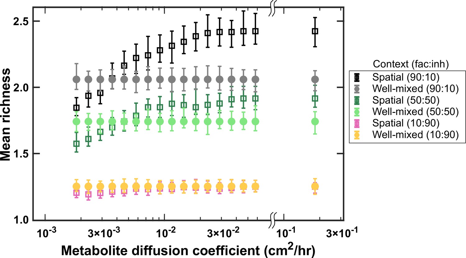
At higher diffusion coefficients of mediators more coexistence is possible.

A range of metabolite diffusion coefficients were simulated in spatial communities (squares) at three different fractions of fac:inh influences (10:90, 50:50, and 90:10). We simulated corresponding well-mixed communities (circles) for comparison. Each condition was run 500 times with the richness (number of species stably surviving at the end of a simulation) averaged over all the simulations. Each simulation started with 10 species and 5 mediators and ran for 100 generations. Other simulation parameters are listed in Table 1. The error bars are 95% confidence intervals generated by bootstrapping 100 samples.

Discussion

Our results dispel the common presumption that a spatially structured environment will universally lead to more coexistence. We find that, compared to a well-mixed environment, a spatial environment can favor or disfavor coexistence depending on the balance between species dispersal and the diffusion of interaction mediators. Interestingly, a lower species dispersal rate favors coexistence, but this effect can be diminished or even reversed if accompanied by low mediator diffusion rates. Coexistence is favored when species have a broad range of consumption and an intermediate range of production of interaction mediators. Additionally, we predict more coexistence when there is a balance between overall production and consumption rates for mediators.

The spatial structure of microbial communities has been extensively studied for example in simulating the development of biofilms (Wang and Zhang, 2010; Kreft et al., 2001; Xavier and Foster, 2007; von der Schulenburg et al., 2009), for specific interactions among species (Momeni et al., 2013b; Momeni et al., 2013a; Kang et al., 2014), or for modeling game-theory dynamics (Nakamaru et al., 1997; Brauchli et al., 1999; Saxer et al., 2009; Hauert and Doebeli, 2004). However, as there is often a tradeoff between the incorporation of detailed mechanisms and generality of conclusions (Levins, 1966; Momeni et al., 2011), we chose in this work to explore a simple, general model of chemically mediated microbial interactions. We assumed, for example, that mediators affected species by additively influencing their growth rates. Although it is possible (and even probable) that mediator effects could be multiplicative, nonlinear, or otherwise context dependent and that they may impact other model parameters, we chose here to present what we felt to be the simplest case. Exploration of alternative implementations of mediator effects would make a fascinating follow-up to this work.

We have made assumptions in our model to simplify the configuration and make the analyses and interpretations easier. We asked if making these assumptions more realistic would affect our conclusions. For example, we have assumed no carrying capacity limit for the growth of our populations. We explored the effect of imposing a total population limit, enforced at each spatial location, and found that it did alter our conclusions (Figure 1—figure supplement 5). However, because the relationship between carrying capacity and coexistence has been explored extensively elsewhere, we chose parameters to minimize this impact, allowing us to focus on other interspecies interactions (beyond competition) and relative rates of diffusion and dispersal. We also tested the impact of the spatial extent of the community (Z), and observed that our results were largely unaffected if the community’s spatial extent was changed by an order of magnitude (Figure 1—figure supplement 4). The effect of larger changes in the spatial extent can be examined by scaling the diffusion and dispersal coefficients accordingly.

Beyond the details of our assumptions, there are also alternative representations of interactions among species, including a simplified Lotka–Volterra model and its variations (Wangersky, 1978), a consumer-resource model (Goldford et al., 2018; Marsland et al., 2019), or a reduced metabolic model (Liao et al., 2020). There are trade-offs in tractability and complexity in choosing which model to use. Our reasoning for adopting the mediator-explicit model was to (1) explicitly include metabolites that mediate the interactions in the model (Momeni et al., 2017); (2) incorporate both metabolites that support the growth of other species as well as those that are inhibitory, such as waste products and toxins (Momeni et al., 2017); and (3) keep the model simple to allow a clear interpretation of mechanisms and processes when analyzing the results. We think it will be worthwhile to compare the predictions of other models to clarify what assumptions are necessary to generate the trends we have obtained and how general the conclusions are.

If spatial organization of cells matters, we also expect that the initial spatial position of species in the community impacts coexistence. To test this, we started from 100 simulations instances and in each case, we tried 100 rearrangements, each obtained by shuffling the spatial position of species, while keeping the species properties and interactions intact. Interestingly, in many cases coexistence was affected (Figure 4—figure supplement 3), indicating that the adjacency to partners is an important determinant of spatial coexistence (as also suggested by Figure 1—figure supplement 3 and Figure 1—figure supplement 7). When we examined the effect of the fac:inh ratio on these outcomes, we observed that larger changes in richness when facilitation interactions were more prevalent in the community (Figure 4—figure supplement 4), which aligns with many of our other results showing that facilitation amplifies the positive effect of spatial structure on coexistence. Although these results are tantalizing, a detailed examination of the spatial organization of populations and metabolites within the community requires a dedicated investigation and is beyond the scope of this work.

Finally, our model assumes that dispersal and diffusion rates are uniform across species and metabolites, respectively. However, dispersal ability can vary widely across microbial taxa, depending on cell size, motility type, chemotaxis, quorum sensing, and other factors. And how the dispersal rates of individuals scale up to affect population- and community-level dynamics is not well understood. Likewise, the diffusion rates of metabolites have the potential to vary greatly with molecule size and shape. Although outside the scope of this work, we are exploring heterogeneity in these rates of movement as an interesting follow-up.

Overall, we believe this work revisits how spatial structure—and spatial self-organization—affects community assembly and coexistence. In our model, which emphasizes the contributions of interspecies interactions, we find that the impact of spatial structure on coexistence largely arises from two processes: (1) spatial self-organization, which can improve coexistence by favoring facilitation over inhibition, and (2) localization of interactions, which can promote coexistence in association with self-organization or hamper coexistence by slowing down and weakening species interactions.

Methods

Model description

Our model is an extension of a model introduced earlier (Niehaus et al., 2019) in which a set of species interact with each other through diffusible mediators. Each mediator is produced by a subset of species, consumed by a subset of species, and has a positive or negative influence on the growth rate of some species (Figure 1).

\begin{array}{cc} \frac{d S_{i} (z, t)}{d t} = D_{C e l l} \frac{d^{2} S_{i} (z, t)}{d z^{2}} \\ + (1 - \frac{\sum_{j = 1}^{M} S_{j} (z, t)}{k_{Y}}) [r_{i 0} + \sum_{j = 1}^{M} ρ_{i j} (\frac{C_{j} (z, t)}{k_{s a t}} δ_{i j}^{-} + \frac{C_{j} (z, t)}{C_{j} (z, t) + k_{s a t}} δ_{i j}^{+})] S_{i} (z, t) \end{array}

\frac{d C_{j} (z, t)}{d t} = D_{M e d} \frac{d^{2} C_{j} (z, t)}{d z^{2}} + \sum_{j = 1}^{M} [β_{j i} S_{i} (z, t) - α_{j i} S_{i} (z, t)]

Here, $S_{i}$ is the spatiotemporal density of species i (i = 1, …, N_c). $C_{j}$ is the spatiotemporal concentration of mediator j (j = 1, …, N_m). D_Cell is the dispersal coefficient for cells. D_Med is the diffusion coefficient for mediators. $k_{Y}$ is the local carrying capacity (for the total density of cells) at each location. $ρ_{i j}$ is the interaction coefficient expressed as the impact of mediator j on species i. Additionally,

δ_{i j}^{-} = {\begin{cases} 1, ρ_{i j} < 0 \\ 0, ρ_{i j} > 0 \end{cases} a n d δ_{i j}^{+} = {\begin{cases} 0, ρ_{i j} < 0 \\ 1, ρ_{i j} > 0 \end{cases}

$k_{s a t}$ is the interaction strength saturation level. $β_{j i}$ and $α_{j i}$ are average production rate and consumption rates, respectively, between species i and mediator j. Similar to Niehaus et al., 2019, each species has a basal growth rate (in the absence of interactions with other species), and influential mediators additively modulate this growth rate. At z = 0 and z = Z, no-flow boundary conditions are enforced for both species and mediators by setting the local spatial derivatives of these parameters to zero at the boundaries.

Typical parameters used in our simulations (unless otherwise stated) are listed in Table 1. These parameters are chosen in the expected realistic range of values; for example, the typical diffusion coefficient of small molecules in water is in the range of 100–1000 µm²/s, and we have used 500 µm²/s as a generic value. When comparing spatial communities with their well-mixed counterparts, exactly the same parameters for basal growth rates, production and consumption rates, mediator influences, and networks of production and consumption are used. This choice is made to reduce the stochasticity caused by other parameters and to focus only on the impact of spatial structure.

Table 1

Parameters used in our simulations are listed.

Parameter	Value (unit)
Number of instances examined ( $N_{s}$ )	500
Number of cell types in the initial pool ( $N_{c}$ )	10
Number of interaction mediators ( $N_{m}$ )	5
Total initial cell density (TID)	10⁴ (cells/ml)
Interaction strength saturation level ( $k_{s a t}$ )	10⁴ (cells/ml)
Population extinction threshold (ExtTh)	0.1 (cells/ml)
Population dilution threshold (DilTh)	10⁷ (cells/ml)
Consumption rate ( $α_{i j}$ )	0.075–2.25 (fmol per cell per hour; avg. 0.15) Stochastic with a uniform distribution
Production rate ( $β_{i j}$ )	0.1–0.2 (fmol per cell per hour; avg. 0.1) Stochastic with a uniform distribution
Probability of production link per population ( $q_{p}$ )	0.5
Probability of influence link per mediator ( $q_{c}$ )	0.5
Maximum interaction strength magnitude ( $r_{i n t, 0}$ )	0.2 (1/hr)
Basal growth rate of species ( $r_{0}$ )	0.1–0.2 (1/hr); stochastic with a uniform distribution
Number of generations for enrichment (nGen)	100
Dispersal coefficient for cells (D_Cell)	5 × 10⁻⁹ (cm²/hr)
Diffusion coefficient for mediators (D_Med)	1.8 × 10⁻² (cm²/hr)
Local carrying capacity per dz (k_Y)	10⁹ cells/ml
Total community spatial extent (Z)	0.5 cm
Spatial resolution for species distributions (dz)	0.005 cm
Cell growth update and uptake timescale (dtau)	0.01 hr
Mediator diffusion time-step (dt)	0.1dz²/D_Med
Cell dispersal simulation time-step (dc)	0.1dz²/D_Cell

To sample different possibilities, the interaction terms as well as production and consumption rates are randomly assigned in each instance of the simulation. Similar to our previous work (Niehaus et al., 2019), the production/consumption matrices are random, that is each element of the matrix has a binomial distribution with a fixed probability of being present ( $q_{p}$ and $q_{c}$ for production and consumption/influence links, respectively). The production and consumption rates have a uniform distribution between 0.5 and 1.5 times a set value each ( $β_{i j}$ and $α_{i j}$ for production and consumption rates, respectively). The interaction matrix which represents the influence of mediators on species has the same structure as the consumption matrix. The magnitude of the influence in this matrix has a uniform distribution between 0 and a maximum value, $r_{i n t, 0}$ . The sign of the influence is chosen from a binomial distribution based on the ratio of fac:inh.

Model implementation

We solve the equations in ‘Model description’ numerically in Matlab using a finite difference discrete version of the equations. Mediator diffusion and cell dispersal take place often at very different time scales. To simulate these processes, we use different numerical time-steps to update the mediator and cell distributions. To allow flexibility in modeling different diffusion and dispersal coefficients, we used asynchronous updates with two independent time-steps: one for updating the diffusion of metabolites and another one for growth and dispersal of cells. The source codes are shared for transparency and reproducibility (see Code availability).

To assess coexistence, we use a criterion similar to Niehaus et al., 2019. In short, any species whose density drops below a pre-specified extinction threshold (ExtTh) is considered extinct. Among species that persist throughout the simulation, only those are considered to coexist whose relative frequency does not decrease by more than 10% of its value in the last 20 generations of the simulation. We consider these species to be ‘stably present’ in the community. Species whose relative frequency declines faster than this threshold are assumed to go extinct later and are not considered to be part of coexisting communities. The only exception to this criterion is the data in Figure 4—figure supplement 1, in which all present species (rather than stably present species) are included in the assessment of final richness.

Statistics

Mean richness values are calculated by averaging the richness values calculated over all simulated instances for a given condition. Confidence intervals for mean richness values are calculated by bootstrapping over all simulated instances for a given condition. The standard routine in Matlab, bootci, is used in all cases for bootstrapping.

Data availability

Codes used to generate the data in this study are shared on GitHub at https://github.com/bmomeni/spatial-coexistence (copy archived at Momeni, 2022).

References

1. Allison SD
(2005) Cheaters, diffusion and nutrients constrain decomposition by microbial enzymes in spatially structured environments
Ecology Letters 8:626–635.
https://doi.org/10.1111/j.1461-0248.2005.00756.x
- Google Scholar
1. Amarasekare P
(2003) Competitive coexistence in spatially structured environments: a synthesis
Ecology Letters 6:1109–1122.
https://doi.org/10.1046/j.1461-0248.2003.00530.x
- Google Scholar
(1999) Evolution of cooperation in spatially structured populations
Journal of Theoretical Biology 200:405–417.
https://doi.org/10.1006/jtbi.1999.1000
- PubMed
- Google Scholar
(2006) Spatial heterogeneity and the stability of host-parasite coexistence
Journal of Evolutionary Biology 19:374–379.
https://doi.org/10.1111/j.1420-9101.2005.01026.x
- PubMed
- Google Scholar
1. Chesson P
(2000a) General theory of competitive coexistence in spatially-varying environments
Theoretical Population Biology 58:211–237.
https://doi.org/10.1006/tpbi.2000.1486
- PubMed
- Google Scholar
1. Chesson P
(2000b) Mechanisms of maintenance of species diversity
Annual Review of Ecology and Systematics 31:343–366.
https://doi.org/10.1146/annurev.ecolsys.31.1.343
- Google Scholar
1. Durrett R
2. Levin S
(1994) The importance of being discrete (and spatial)
Theoretical Population Biology 46:363–394.
https://doi.org/10.1006/tpbi.1994.1032
- Google Scholar
1. Durrett R
2. Levin S
(1998) Spatial aspects of interspecific competition
Theoretical Population Biology 53:30–43.
https://doi.org/10.1006/tpbi.1997.1338
- PubMed
- Google Scholar
Book
1. Gause GF
(1934) The Struggle for Existence
Williams & Wilkins.
https://doi.org/10.5962/bhl.title.4489
- Google Scholar
1. Goldford JE
2. Lu N
3. Bajić D
4. Estrela S
5. Tikhonov M
6. Sanchez-Gorostiaga A
7. Segrè D
8. Mehta P
9. Sanchez A
(2018) Emergent simplicity in microbial community assembly
Science 361:469–474.
https://doi.org/10.1126/science.aat1168
- Google Scholar
1. Hauert C
2. Doebeli M
(2004) Spatial structure often inhibits the evolution of cooperation in the snowdrift game
Nature 428:643–646.
https://doi.org/10.1038/nature02360
- PubMed
- Google Scholar
1. Kang S
2. Kahan S
3. Momeni B
(2014) Simulating microbial community patterning using Biocellion
Methods in Molecular Biology 1151:233–253.
https://doi.org/10.1007/978-1-4939-0554-6_16
- PubMed
- Google Scholar
(2002) Local dispersal promotes biodiversity in a real-life game of rock-paper-scissors
Nature 418:171–174.
https://doi.org/10.1038/nature00823
- PubMed
- Google Scholar
(2008) Defined spatial structure stabilizes a synthetic multispecies bacterial community
PNAS 105:18188–18193.
https://doi.org/10.1073/pnas.0807935105
- PubMed
- Google Scholar
1. Kim HJ
2. Du W
3. Ismagilov RF
(2011) Complex function by design using spatially pre-structured synthetic microbial communities: degradation of pentachlorophenol in the presence of Hg(Ii)
Integrative Biology 3:126–133.
https://doi.org/10.1039/c0ib00019a
- PubMed
- Google Scholar
(2001) Individual-based modelling of biofilms
Microbiology 147:2897–2912.
https://doi.org/10.1099/00221287-147-11-2897
- PubMed
- Google Scholar
(2014) Habitat structure and the evolution of diffusible siderophores in bacteria
Ecology Letters 17:1536–1544.
https://doi.org/10.1111/ele.12371
- PubMed
- Google Scholar
1. Levins R
(1966)
The strategy of model building in population biology

American Scientist 54:421–431.
- Google Scholar
1. Liao C
2. Wang T
3. Maslov S
4. Xavier JB
(2020) Modeling microbial cross-feeding at intermediate scale portrays community dynamics and species coexistence
PLOS Computational Biology 16:e1008135.
https://doi.org/10.1371/journal.pcbi.1008135
- PubMed
- Google Scholar
1. Ma B
2. Wang Y
3. Ye S
4. Liu S
5. Stirling E
6. Gilbert JA
7. Faust K
8. Knight R
9. Jansson JK
10. Cardona C
11. Röttjers L
12. Xu J
(2020) Earth microbial co-occurrence network reveals interconnection pattern across microbiomes
Microbiome 8:82.
https://doi.org/10.1186/s40168-020-00857-2
- PubMed
- Google Scholar
1. Marsland R
2. Cui W
3. Goldford J
4. Sanchez A
5. Korolev K
6. Mehta P
(2019) Energy fluxes drive a transition in the diversity, stability, and functional structure of microbial communities
PLOS Computational Biology 15:e1006793.
https://doi.org/10.1371/journal.pcbi.1006793
- PubMed
- Google Scholar
1. Momeni B
2. Chen CC
3. Hillesland KL
4. Waite A
5. Shou W
(2011) Using artificial systems to explore the ecology and evolution of symbioses
Cellular and Molecular Life Sciences 68:1353–1368.
https://doi.org/10.1007/s00018-011-0649-y
- PubMed
- Google Scholar
1. Momeni B
2. Brileya KA
3. Fields MW
4. Shou W
(2013a) Strong inter-population cooperation leads to partner Intermixing in microbial communities
eLife 2:e00230.
https://doi.org/10.7554/eLife.00230
- PubMed
- Google Scholar
1. Momeni B
2. Waite AJ
3. Shou W
(2013b) Spatial self-organization favors heterotypic cooperation over cheating
eLife 2:e00960.
https://doi.org/10.7554/eLife.00960
- PubMed
- Google Scholar
1. Momeni B
2. Xie L
3. Shou W
(2017) Lotka-Volterra Pairwise modeling fails to capture diverse pairwise microbial interactions
eLife 6:e25051.
https://doi.org/10.7554/eLife.25051
- PubMed
- Google Scholar
Software
1. Momeni B
(2022) Spatial-coexistence, version swh:1:rev:22ccb5cb7fa51823068f24ee7bfc232a87ca6350
Software Heritage.

https://archive.softwareheritage.org/swh:1:dir:82dde7c8414fb422837472b039e9f62edd42b7d7;origin=https://github.com/bmomeni/spatial-coexistence;visit=swh:1:snp:7d7f511cc27e43577eb122f413df51ad4e770d8e;anchor=swh:1:rev:22ccb5cb7fa51823068f24ee7bfc232a87ca6350
1. Murrell DJ
2. Law R
(2003) Heteromyopia and the spatial coexistence of similar competitors
Ecology Letters 6:48–59.
https://doi.org/10.1046/j.1461-0248.2003.00397.x
- Google Scholar
(2016) Spatial structure, cooperation and competition in biofilms
Nature Reviews. Microbiology 14:589–600.
https://doi.org/10.1038/nrmicro.2016.84
- PubMed
- Google Scholar
(1997) The evolution of cooperation in a lattice-structured population
Journal of Theoretical Biology 184:65–81.
https://doi.org/10.1006/jtbi.1996.0243
- PubMed
- Google Scholar
1. Niehaus L
2. Boland I
3. Liu M
4. Chen K
5. Fu D
6. Henckel C
7. Chaung K
8. Miranda SE
9. Dyckman S
10. Crum M
11. Dedrick S
12. Shou W
13. Momeni B
(2019) Microbial coexistence through chemical-mediated interactions
Nature Communications 10:2052.
https://doi.org/10.1038/s41467-019-10062-x
- PubMed
- Google Scholar
1. Pande S
2. Kaftan F
3. Lang S
4. Svatoš A
5. Germerodt S
6. Kost C
(2016) Privatization of cooperative benefits stabilizes mutualistic cross-feeding interactions in spatially structured environments
The ISME Journal 10:1413–1423.
https://doi.org/10.1038/ismej.2015.212
- PubMed
- Google Scholar
1. Satoh H
2. Miura Y
3. Tsushima I
4. Okabe S
(2007) Layered structure of bacterial and archaeal communities and their in situ activities in anaerobic granules
Applied and Environmental Microbiology 73:7300–7307.
https://doi.org/10.1128/AEM.01426-07
- PubMed
- Google Scholar
(2009) Spatial structure leads to ecological breakdown and loss of diversity
Proceedings of the Royal Society B 276:2065–2070.
https://doi.org/10.1098/rspb.2008.1827
- Google Scholar
Book
1. Solé RV
2. Bascompte J
(2006) Self-Organization in Complex Ecosystems
Princeton University Press.
https://doi.org/10.1515/9781400842933
- Google Scholar
1. Tilman D
(1990) Constraints and tradeoffs: toward a predictive theory of competition and succession
Oikos 58:3.
https://doi.org/10.2307/3565355
- Google Scholar
1. Tilman D
(1994) Competition and biodiversity in spatially structured Habitats
Ecology 75:2–16.
https://doi.org/10.2307/1939377
- Google Scholar
Book
1. Tilman D
2. Kareiva P
(1998) Spatial Ecology
Princeton University Press.
https://doi.org/10.1515/9780691188362
- Google Scholar
(2009) Three-dimensional simulations of biofilm growth in porous media
AIChE Journal 55:494–504.
https://doi.org/10.1002/aic.11674
- Google Scholar
1. Wang Q
2. Zhang T
(2010) Review of mathematical models for biofilms
Solid State Communications 150:1009–1022.
https://doi.org/10.1016/j.ssc.2010.01.021
- Google Scholar
1. Wangersky PJ
(1978) Lotka-Volterra population models
Annual Review of Ecology and Systematics 9:189–218.
https://doi.org/10.1146/annurev.es.09.110178.001201
- Google Scholar
(2019) Spatial ecology of territorial populations
PNAS 116:17874–17879.
https://doi.org/10.1073/pnas.1911570116
- PubMed
- Google Scholar
1. Widder S
2. Allen RJ
3. Pfeiffer T
4. Curtis TP
5. Wiuf C
6. Sloan WT
7. Cordero OX
8. Brown SP
9. Momeni B
10. Shou W
11. Kettle H
12. Flint HJ
13. Haas AF
14. Laroche B
15. Kreft J-U
16. Rainey PB
17. Freilich S
18. Schuster S
19. Milferstedt K
20. van der Meer JR
21. Groβkopf T
22. Huisman J
23. Free A
24. Picioreanu C
25. Quince C
26. Klapper I
27. Labarthe S
28. Smets BF
29. Wang H
30. Isaac Newton Institute Fellows
31. Soyer OS
(2016) Challenges in microbial ecology: building predictive understanding of community function and dynamics
The ISME Journal 10:2557–2568.
https://doi.org/10.1038/ismej.2016.45
- PubMed
- Google Scholar
1. Xavier JB
2. Foster KR
(2007) Cooperation and conflict in microbial biofilms
PNAS 104:876–881.
https://doi.org/10.1073/pnas.0607651104
- PubMed
- Google Scholar

Decision letter

Sara Mitri

Reviewing Editor; University of Lausanne, Switzerland
Detlef Weigel

Senior Editor; Max Planck Institute for Biology Tübingen, Germany
Daniel R Amor

Reviewer; University of Graz, Austria

Our editorial process produces two outputs: (i) public reviews designed to be posted alongside the preprint for the benefit of readers; (ii) feedback on the manuscript for the authors, including requests for revisions, shown below. We also include an acceptance summary that explains what the editors found interesting or important about the work.

Decision letter after peer review:

Thank you for submitting your article "Spatial structure may favor or disfavor microbial coexistence" for consideration by eLife. Your article has been reviewed by 3 peer reviewers, and the evaluation has been overseen by a Reviewing Editor and Naama Barkai as the Senior Editor. The following individuals involved in the review of your submission have agreed to reveal their identity: Daniel R Amor (Reviewer #1).

The reviewers have discussed their reviews with one another, and the Reviewing Editor has drafted this to help you prepare a revised submission.

Essential revisions:

As you can read in more detail below, the three reviewers all made similar recommendations to improve your manuscript. Please address at least the following points:

1) Justify the definition of coexistence (the 90% threshold);

2) Justify the way dispersal is implemented and the choice of diffusion coefficients;

3) Check for typos in the equations and the implementation of the carrying capacity;

4) Explore how relaxing these assumptions or using more realistic parameter values would affect current conclusions;

5) Explore not only coexistence but also population composition and the resulting spatial patterns.

Reviewer #1 (Recommendations for the authors):

I present here more concrete suggestions and concerns related to my comments in the public review.

1. I believe that there might be some errors in how the model's equations for species dynamics (line 298) were written in the manuscript. In the equation in line 299, should the term above the total cell carrying capacity (Ky) be a sum of all the species abundances instead of all the metabolites abundances? I believe that this is not the way that the matlab code was implemented, but it would be worth it for the authors to double-check this in all the scripts.

Ksat should have the same units as Cj(z,t), which is in disagreement with the units proposed in table 1. Similarly, Ky should have the same units as Si(z,t). Furthermore, it was not very clear how interactions, production, and consumption rates were assigned. Do they exist with a certain probability and, provided that they exist, their strength is sampled from a uniform distribution?

2. Line 321 defines the criteria to determine coexistence: 'only those with relative frequencies equal to or larger than 90% of the fastest growing species in the last 20 generations of the simulation are considered to coexist'. I am surprised by the relatively high (90%) threshold. This means that a pair of species that reaches a stable equilibrium of e.g. 10^7cells/ mL and 8*10^6 cells/mL is not classified as a pair of coexisting species. Please, discuss why the criteria imply such a high evenness of species abundances (experimental measures often report stable coexistence of species at many different fractions). I wonder if relaxing this strong requirement would significantly affect the results of community richness.

3. The text should be more clear from the beginning that the 'slow dispersal' scenario that is analyzed through the first sections (Figures1-3) is qualitatively very similar to a 'zero dispersal' scenario. Just to illustrate why I think this, one can use the Fisher's front speed solution v = 2*sqrt (r*D) to have an estimate (based on the proposed parameter values) of how much distance a monoculture could travel in the absence of interactions. The result, taking into account the timescale of the simulations (~350 hr, assuming r0 = 0.2/hr), is a total distance of ~0.02cm, which is consistent with the results in Figure S2. This means that, in this regime, microbial dynamics are mostly driven by growth, not by dispersal. On the other hand, considering the value of D in the 'fast dispersal' scenario gives an approximate front speed of 2*10^(-3)cm/hr (travelling ~0.7cm in 350 hours) for a monoculture in the absence of interactions. This is closer to observed speeds for colonies of non-motile bacteria growing on hard agar, and still falls on the slower end for such speeds. If one thinks about motile bacteria in soft agar, the speeds are even faster. Overall, I wonder about the kind of system that the 'slow dispersal' scenario could be modelling and, more importantly, whether the authors would consider analyzing the implications of 'fast dispersal' scenarios in more depth. How would Figures2 and 3 look under fast dispersal?

4. The figures of the main text could incorporate more analysis and results that further support the main message of each figure. Most of the figures contain only one panel (or one type of panel) and further information on the many parameters that could affect that result is left to the Supplementary Information. In some cases, just bringing some of the supplementary analysis to the main figures would make them more comprehensive while increasing the readability of the paper. Just to give some examples, figure 1 could incorporate the cartoon that explains the model (Figure S1), a time series, and some spatial profiles of species abundances to illustrate the typical dynamics of the system (e.g. incorporate some of the data in Figure S2). More snapshots of spatial profiles would help understand what happens in different scenarios, e.g. in Figure S6. In figures 2 and 3, how do these results depend on the average interaction strength (growth rate impact) of metabolites-to-bacteria?

5. The work will benefit from the additional analysis that can strengthen certain interpretations of the current results. For example, Figure S5 shows the dependence of species richness on the carrying capacity of the system. The authors claim that a shift towards intraspecies competition is responsible for such dependence and that a limited carrying capacity suppresses the more competitive species, but no statistical analysis on individual species performance is provided to back this argument (and species competitiveness is lacking a working definition). The criteria to determine the length of the simulations is another example, the authors said that 100 generations are 'often' enough to reach stability, but a more rigorous analysis or definition of stability would be better. Regarding the statement in line 116, an analysis of how much better or worse species grow when close to facilitative/inhibitory partners would be helpful.

6. The lack of analysis/visualization of spatial profiles for metabolite abundances leaves the reader wondering about the spatial scale of the interactions. Some representative cases could appear in the supplement, or be incorporated into one of the main figures.

Reviewer #2 (Recommendations for the authors):

The authors extend a mathematical model that they previously developed (Niehaus..Momeni, Nature Comm., 2019) for the study of microbial communities growing in well-mixed settings, to the case where species grow in spatial settings. They find that spatial structure promotes the coexistence of species when interactions are more facilitating than inhibiting, and when species dispersal is low. We found the paper well-written and well-organized. However, we have a number of comments: the main contribution of the paper is to extend a well-mixed model to a spatial model; It is thus fundamental that the assumptions made by the authors to model the spatial dynamics are well justified; we think that several physical parameters are chosen to values that do not represent realistic values for spatially structured communities and that the authors should discuss if the results hold also for more realistic values.

Line 84: The Authors state that they start each simulation from an initial distribution in which populations occupy adjacent, overlapping spatial locations at low initial density. What is the variation in the steady state distribution of species if they run many simulations with the same initial state and with the same parameters?

Line 88: "We have chosen 100 generations of growth because we have observed that often this is enough to reliably decide which species stably persist in the community." We think that the concept of generation is not clear. Can the authors define what generation means exactly? Also, can they provide a quantification for "reliably" when they say that the system converges reliably?

Line 91: The authors define a specific dilution procedure. We do not understand how they motivate this specific choice of dilution procedure. At each dilution step, they assume that the overall spatial distribution of the community is preserved and all populations at all locations are diluted by the same factor. Regarding this assumption, the authors say that they "adopt it as the least biased possibility, in the absence of additional information about a particular community." We have two questions regarding this assumption:

i) Is this really the least biased assumption? We suggest that a random distribution of the initial species is more a null model than the current choice. Or is there a reason to think that cells forming a new community by default inherit the spatial configuration of the parent community?

ii) Do the authors have a natural mechanism of community propagation in mind that they could refer to, which would correspond to their assumption?

Having in mind the concept of metacommunities, we don't understand how spatial distribution can be inherited by the new community.

Line 101: The authors say that a shift from competition to competition can favor coexistence in a spatially structured environment. When doing this analysis, the authors impose a cap on the total cell number that can exist at each location in space. The more restrictive the cap is, the more coexistence they find.

Regarding this conclusion, we would like the author to comment on the choice of the cap. The cap they pick is 10^9 cells/ml. This density is quite a low density for a spatially structured system. A back-of-the-envelope calculation can show that at 10^9 cells/ml, the volume ratio between cells and environment is 1:1000, if we consider that a cell occupies approximately 1 μm cube (e.g. E. coli in Minimal media+glucose is about that size. See: https://www.ncbi.nlm.nih.gov/books/NBK224751/). These are the order of magnitude estimates of course, but they suggest that the authors use a density that is much lower than expected in a spatially structured community, like a biofilm. In fact,10^9 cells/ml is about the density of cells in an overnight of E. coli grown in Minimal media (M9) with 0.2% glucose. We would suggest picking values closer to a dense community, and our expectation is that spatially structured communities should be at least 10^11 cells/ml. Following the calculation above, this would lead to a volume ratio between cells and the environment of 1:10, if we consider that a cell occupies 1 μm cube.

We would like the authors to comment on the following two points:

i) Why do they pick 10^9 cells/ml as a maximum cap, which seems such a low density?

ii) The authors pick 10^9 cells/ml because this cap maximizes coexistence. In light of the calculation we do here, what would happen if they used higher values of cell densities?

Line 101: 10^9 cells/ml is not 10^9 cells/cm as stated in Table 1. Can we think of these units as being the same? If yes, can units be homogenized? At the moment most of the units suggest that the effective dynamics is a 3D dynamics (e.g. diffusion constants, densities of cells), even if then they implement a 1D world, where there exists a line of "cubes" filled with sub-communities.

Table 1: The authors state that "Diffusion coefficient for mediators (DMed) 1.8 10-3 (cm2/hr)".

Again we do not understand the choice of parameters. When we look at realistic values of molecules diffusing, we see that these are more than 10 times faster. Here are two examples for glucose and for one amino acid:

For Glucose, the diffusion constant in water is 600 um^2 /sec, which is about 21*10-3 cm2/hr. See: https://bionumbers.hms.harvard.edu/bionumber.aspx?s=n&v=7&id=104089

For amino acids, the diffusion constant in water is 800 um^2/sec. See Wu, Y., Ma, P., Liu, Y. & Li, S. Diffusion coefficients of l-proline, l-threonine and l-arginine in aqueous solutions at 25◦C. Fluid Phase Equilibria 186, 27-38 (2001).

Table 1: Can they comment on the value of diffusion of species? This value represents somehow a fraction of individuals that move away from the local patch into another patch. What should we think this fraction to be?

Figure 1: what is the explanation for which, at a low fraction of facilitative interactions, coexistence in well-mixed and spatial communities is the same? Can they comment on this?

Figure 5: Do the authors expect that by increasing diffusion even further, coexistence should decrease again? Does the exploration stop at the maximum diffusion expected in liquid?

Reviewer #3 (Recommendations for the authors):

– I think there is a typo in the equations shown in the "Model description" section. In the population dynamics equation, the carrying capacity term (the one with k_Y) appears to contain a sum over the C_j rather than the expected sum over the S_i. In the supplied code, it appears that this term sums over the populations.

– Assuming the carrying capacity term is meant to contain a sum over the S_i rather than the C_j, the current formulation of this model may lead to non-physical outcomes. Consider a population that is above carrying capacity, such that the carrying capacity term is negative. If this population is also surrounded by highly detrimental chemical mediators (such that its interaction term is negative), the product of the negative carrying capacity and interaction terms will result in a positive growth rate. From the code I have looked at (Spatial1DInteraction_DpMM_ExMTC_flexibleTimeStep.m, lines 103-110), there doesn't seem to be any mechanism to prevent this. However, from the supplementary plots, it does not appear that the steady-state population abundances exceed the k_Y. The authors should assess whether these non-physical dynamics occur in their simulations, as it could artificially inflate coexistence. One possible solution is to set the population growth to zero if the carrying capacity is exceeded.

– One limitation of the authors' current analyses is that it is based only on richness, which does not reflect population abundance. Equivalent comparisons between the spatial and non-spatial models could be made with a metric like the Shannon entropy, which does consider population abundance. To compute the Shannon entropy in the spatial model, one could measure the total population of each cell type by integrating over the domain. From these abundances, a relative abundance distribution compatible with the Shannon entropy could be calculated. It would be worthwhile to assess whether the observed trends are similar when other metrics are used.

– I think it would be worthwhile for the authors to quantify the spatial patterns of coexistence in their model. I understand the authors' reasoning for focusing on a metric that does not consider spatial structure, as such metrics are the only ones that can be used to compare directly between spatial and well-mixed systems. However, from the plots shown in Figure S2, it appears that coexistence in this model can manifest as quite non-trivial spatial patterns. Spatial coexistence patterns of natural microbial communities are often strikingly beautiful, and it would be interesting to assess how this model's parameters influence its resulting spatial coexistence patterns. For example, one could examine the relationship between the mediator and microbe diffusion rates and the size/overlap of microbial domains, or analyze the existence of the seeming "dead-zones" of the domain seen in the bottom right panel of Figure S2.

– I find the result that changing the order of species in the initial condition can change the final richness to be very interesting (Figure S8). This result implies that there is a great deal of multistability in the dynamics. In a metapopulation context, this could be its own diversity-generating mechanism. I think discussing this multistability more explicitly in the main text would be worthwhile: is this multistability a result of spatial dynamics?

– The authors should specify the distribution of mediator production/consumption and interaction coefficients. Currently, I'm not sure what distribution these parameters are drawn from.

– In the figures with well-mixed vs. spatial heatmaps, it may be worthwhile to include a plot that directly depicts the ratio of the two model's richness values. As it stands, I found it a bit difficult to immediately see the differences between the well-mixed and spatial results.

https://doi.org/10.7554/eLife.82504.sa1

Author response

Essential revisions:

As you can read in more detail below, the three reviewers all made similar recommendations to improve your manuscript. Please address at least the following points:

1) Justify the definition of coexistence (the 90% threshold);

As explained below in response to reviewers’ comments, in our definition of coexistence, we assess the changes in the relative frequency of species in the last 20 generations (compared to the fastest growing species) of our simulations. If the relative frequency of a species drops by more than 10% within 20 generations, we assume that they are destined to go extinct in the long-term. The idea is to eliminate species that are slowly going extinct, but are still present after 100 generations (the typical extent of each of our simulations). To be clear, there is no threshold on the steady state relative frequency of each species; i.e. the ratio of fastest growing to slowest growing coexisting species can be 1e6:1, 1:1, or 1:1e6, as long as the ratio does not change considerably during the last 20 generations of our simulations. We have reworded the sentence to 'only those species whose relative frequency do not drop by more than 10% compared to the fastest growing species in the last 20 generations of the simulation are considered to coexist.' We have also included Figure 4—figure supplement 1 as an example of a modified criterion to examine the final richness based on which species are present, rather than which species are stably present.

2) Justify the way dispersal is implemented and the choice of diffusion coefficients;

The primary reason for choosing the dispersal coefficients to be relatively small was to maintain the spatial structure of the community. This choice was made to highlight how spatial structure can contribute to coexistence. Our vision of an example of a community being discussed was a microbial mat in which there can be dispersal but a strong stratification is maintained. We agree with the reviewers that including a wider range of parameters would be informative; we have thus expanded our scope and included a wider range of parameters (including higher dispersal rates) in the revised version.

3) Check for typos in the equations and the implementation of the carrying capacity;

Thank you for pointing this out. The typo is fixed in the revised version.

4) Explore how relaxing these assumptions or using more realistic parameter values would affect current conclusions;

Our focus here is on general concepts, based on the relative rates of mediator diffusion and cell dispersal, rather than on attempting to recreate a particular community. Nevertheless, the choices made about the parameters are such that they are relevant to some examples of microbial communities such as microbial mats. We have included additional sentences to the introduction section to make it clear that in this paper we examine different ranges of parameters (some of them intentionally close to extremes) to explore different mechanisms and general principles.

5) Explore not only coexistence but also population composition and the resulting spatial patterns.

To address this comment, we have added more instances of spatial patterns of the communities along with coexistence results. We have also used Shannon index as a measure of evenness of the community in some of our comparisons of well-mixed versus spatial communities. We would like to emphasize that a detailed examination of the spatial organization of populations and metabolites within the community requires a dedicated investigation and is beyond the scope of this work. We plan to address these spatial organization aspects in future work.

Reviewer #1 (Recommendations for the authors):

I present here more concrete suggestions and concerns related to my comments in the public review.

1. I believe that there might be some errors in how the model's equations for species dynamics (line 298) were written in the manuscript. In the equation in line 299, should the term above the total cell carrying capacity (Ky) be a sum of all the species abundances instead of all the metabolites abundances? I believe that this is not the way that the matlab code was implemented, but it would be worth it for the authors to double-check this in all the scripts.

Ksat should have the same units as Cj(z,t), which is in disagreement with the units proposed in table 1. Similarly, Ky should have the same units as Si(z,t). Furthermore, it was not very clear how interactions, production, and consumption rates were assigned. Do they exist with a certain probability and, provided that they exist, their strength is sampled from a uniform distribution?

Thank you for pointing out the typo. You are correct, that term is in fact the sum of all species abundances and we have confirmed that this was correctly implemented in our simulation codes in Matlab. We have fixed the Equation in the revised version.

We have added the following paragraph to clarify how the interactions and production/consumption rates were assigned (lines 393-402):

“To sample different possibilities, the interaction terms as well as production and consumption rates are randomly assigned in each instance of the simulation. Similar to our previous work [25], the production/consumption matrices are random, i.e. each element of the matrix has a binomial distribution with a fixed probability of being present (q_p and q_c for production and consumption/influence links, respectively). The production rate and consumption rates have a uniform distribution between 0.5 and 1.5 times a set value each (β_ij and α_ij for production and consumption rates, respectively). The interaction matrix which represents the influence of mediators on species has the same structure as the consumption matrix. The magnitude of the influence in this matrix has a uniform distribution between 0 and a maximum value, r_int,0. The sign of the influence is chosen from a binomial distribution based on the ratio of fac:inh.”

2. Line 321 defines the criteria to determine coexistence: 'only those with relative frequencies equal to or larger than 90% of the fastest growing species in the last 20 generations of the simulation are considered to coexist'. I am surprised by the relatively high (90%) threshold. This means that a pair of species that reaches a stable equilibrium of e.g. 10^7cells/ mL and 8*10^6 cells/mL is not classified as a pair of coexisting species. Please, discuss why the criteria imply such a high evenness of species abundances (experimental measures often report stable coexistence of species at many different fractions). I wonder if relaxing this strong requirement would significantly affect the results of community richness.

Sorry for the confusion. The 90% threshold applies to the changes in the relative frequency in the last 20 generations compared to the fastest growing species. Coexisting species can have any relative frequency compared to each other (1:1 or 1:10⁶) in terms of the composition of the community. However, if the relative frequency of a population drops by more than 10% in 20 generations, we assume that they are destined to go extinct in the long-term. The idea is to eliminate species that are slowly going extinct, but are still present after 100 generations which is the typical extent of each run. We have reworded the sentence to the following (lines 412-420):

“To assess coexistence, we use a criterion similar to [25]. In short, any species whose density drops below a pre-specified extinction threshold (ExtTh) is considered extinct. Among species that persist throughout the simulation, only those with relative frequencies equal to or larger than 90% of the fastest growing species in the last 20 generations of the simulation are considered to coexist. We consider these species to be ‘stably present’ in the community. Species with a declining relative frequency are assumed to go extinct later and are not considered to be part of coexisting communities. The only exception to this criterion is the data in Figure 4—figure supplement 1, in which all ‘present’ species (rather than stably present species) are included in the assessment of final richness.”

We have also changed the terminology to call species that satisfy this criterion and coexist in a community as ‘stably present’ to make the distinction clearer.

3. The text should be more clear from the beginning that the 'slow dispersal' scenario that is analyzed through the first sections (Figures1-3) is qualitatively very similar to a 'zero dispersal' scenario. Just to illustrate why I think this, one can use the Fisher's front speed solution v = 2*sqrt (r*D) to have an estimate (based on the proposed parameter values) of how much distance a monoculture could travel in the absence of interactions. The result, taking into account the timescale of the simulations (~350 hr, assuming r0 = 0.2/hr), is a total distance of ~0.02cm, which is consistent with the results in Figure S2. This means that, in this regime, microbial dynamics are mostly driven by growth, not by dispersal. On the other hand, considering the value of D in the 'fast dispersal' scenario gives an approximate front speed of 2*10^(-3)cm/hr (travelling ~0.7cm in 350 hours) for a monoculture in the absence of interactions. This is closer to observed speeds for colonies of non-motile bacteria growing on hard agar, and still falls on the slower end for such speeds. If one thinks about motile bacteria in soft agar, the speeds are even faster. Overall, I wonder about the kind of system that the 'slow dispersal' scenario could be modelling and, more importantly, whether the authors would consider analyzing the implications of 'fast dispersal' scenarios in more depth. How would Figures2 and 3 look under fast dispersal?

We agree with the reviewer about the range of dispersal represented in Figures1-3. The low dispersal regime was initially chosen as a way to make a clear distinction from the well-mixed condition and exaggerate the spatial aspects. We would like to emphasize that even changes in this regime, which would be perhaps considered minor differences in motility, still have an impact on coexistence. We have included additional results of ‘fast dispersal’ in the supplementary information of the revised manuscript (Figure 1—figure supplement 2). We have also expanded Figure 4 to include ‘fast dispersal’ and added the corresponding discussions and two supplementary figures (Figure 4—figure supplement 1 and Figure 4—figure supplement 2) in the revised manuscript (lines 236-274).

“At intermediate levels of dispersal, the trend reversed and well-mixed communities showed more coexistence compared to spatial communities. This is interesting because at the limit of extremely rapid diffusion (shown with a ‘∞’ sign in Figure 4) when we kept the species distribution uniform across the spatial extent, coexistence outcomes matched the well-mixed case, as expected. We found two factors that contributed to this trend. The first contribution came from longer-term changes in dynamics at intermediate levels of dispersal. Even after 100 generations, which is the typical extent of our studies, at intermediate levels of dispersal (e.g. DCell = 5×10-6 cm2/hr), the spatial distribution of populations is still changing considerably. As a result, our strict criteria for stable coexistence removes some of the populations that are still temporally not stable enough, leading to a lower overall assessment of coexistence in these cases. To show this, we examined the range of dispersal coefficients again, but kept all the species that were present after 100 generations, rather than those with stable population fractions at that point (see Model implementation in Methods). The results show that higher dispersal coefficients using this measure lowers the richness of resulting communities (based on presence, rather than stable presence), but not below the levels expected from well-mixed communities (Figure 4—figure supplement 1). As a second factor, we hypothesized that self-facilitation interactions contribute to the decrease in coexistence at intermediate dispersal levels. Our rationale was that self-facilitation interactions are amplified in communities in which the spatial context is preserved, because the distribution of producers matches the distribution of self, but not other recipients in such a case. This can lead to community overtake by a self-facilitating species. This effect will be weaker in communities at intermediate dispersal rates: at low dispersal rates self-facilitating species will be more confined in space and some of the metabolite will leak out to other species; in the other extreme, in the very high dispersal rates all distributions will become uniform and the distinction between self and others diminishes. To test this, we tested weaker self-facilitation links in our simulations and observed that this change led to higher coexistence in communities with intermediate dispersal coefficients but not in well-mixed communities or communities with low dispersal coefficients (Figure 4—figure supplement 2). It is a matter of debate how prevalent self-facilitation interactions are within microbial communities. Self-facilitation interactions do exist, for example when a species breaks down a recalcitrant substrate such as cellulose into smaller molecules that can be beneficial. However, if they are not as prevalent as what our model assumes, some of our predictions might be affected.”

4. The figures of the main text could incorporate more analysis and results that further support the main message of each figure. Most of the figures contain only one panel (or one type of panel) and further information on the many parameters that could affect that result is left to the Supplementary Information. In some cases, just bringing some of the supplementary analysis to the main figures would make them more comprehensive while increasing the readability of the paper. Just to give some examples, figure 1 could incorporate the cartoon that explains the model (Figure S1), a time series, and some spatial profiles of species abundances to illustrate the typical dynamics of the system (e.g. incorporate some of the data in Figure S2). More snapshots of spatial profiles would help understand what happens in different scenarios, e.g. in Figure S6. In figures 2 and 3, how do these results depend on the average interaction strength (growth rate impact) of metabolites-to-bacteria?

Thank you for the suggestion. We have combined former Figure S1 with Figure 1, in response to your suggestion. To make the relevant figures more accessible, we have also renamed the supplementary figures as Figure 1-S1, Figure 1-S2, etc. to take advantage of the eLife format that aggregates all supplementary figures related to each main figure. We believe this format will make it easier for the reader to see additional aspects related to the message of each figure (which are provided in supplementary figures).

We have also added supplementary figures to show that the trends in Figures2 and 3 are preserved at weaker and stronger interaction levels (Figure 2—figure supplement 2, Figure 2—figure supplement 3, Figure 3figure supplement 2, and Figure 3—figure supplement 3).

Figure 1—figure supplement 3 in the revised version addresses your concern about more snapshots of the spatial profile by comparing the low-dispersal and high-dispersal cases.

5. The work will benefit from the additional analysis that can strengthen certain interpretations of the current results. For example, Figure S5 shows the dependence of species richness on the carrying capacity of the system. The authors claim that a shift towards intraspecies competition is responsible for such dependence and that a limited carrying capacity suppresses the more competitive species, but no statistical analysis on individual species performance is provided to back this argument (and species competitiveness is lacking a working definition). The criteria to determine the length of the simulations is another example, the authors said that 100 generations are 'often' enough to reach stability, but a more rigorous analysis or definition of stability would be better. Regarding the statement in line 116, an analysis of how much better or worse species grow when close to facilitative/inhibitory partners would be helpful.

To show our rationale behind the choice of 100 generations as a representative time for the outcome of the communities, we have added a supplementary figure (Figure 1—figure supplement 1). It demonstrates that the community composition after 100 generations typically only undergoes small fluctuations in both well-mixed and spatial communities.

Regarding the statement in line 116, we have added Figure 1—figure supplement 6 as an example of commensalism when the distance between the provider and recipient was changed. In this example, the benefit received depended on the diffusion of the mediator. As a result, stronger interaction was observed when species are closer to each other.

6. The lack of analysis/visualization of spatial profiles for metabolite abundances leaves the reader wondering about the spatial scale of the interactions. Some representative cases could appear in the supplement, or be incorporated into one of the main figures.

Thank you for the suggestion. We have added more representative cases of both spatial patterns (Figure 1—figure supplement 3) and community dynamics (Figure 1—figure supplement 4 and Figure 1—figure supplement 5) in the revised version of the manuscript.

Reviewer #2 (Recommendations for the authors):

The authors extend a mathematical model that they previously developed (Niehaus..Momeni, Nature Comm., 2019) for the study of microbial communities growing in well-mixed settings, to the case where species grow in spatial settings. They find that spatial structure promotes the coexistence of species when interactions are more facilitating than inhibiting, and when species dispersal is low. We found the paper well-written and well-organized. However, we have a number of comments: the main contribution of the paper is to extend a well-mixed model to a spatial model; It is thus fundamental that the assumptions made by the authors to model the spatial dynamics are well justified; we think that several physical parameters are chosen to values that do not represent realistic values for spatially structured communities and that the authors should discuss if the results hold also for more realistic values.

Thank you for your constructive feedback. We have revised the manuscript to explain the model assumptions and fixed some of the errors that had created the impression that the model parameters were not realistic.

Line 84: The Authors state that they start each simulation from an initial distribution in which populations occupy adjacent, overlapping spatial locations at low initial density. What is the variation in the steady state distribution of species if they run many simulations with the same initial state and with the same parameters?

With the same initial state and the same parameters, the simulations are deterministic and there is no stochasticity in the results. The stochasticity is intentionally introduced in the properties of the species (e.g. basal growth rates, rates of consumption and production, etc.) to assess the outcomes in many instances of simulated communities.

Line 88: "We have chosen 100 generations of growth because we have observed that often this is enough to reliably decide which species stably persist in the community." We think that the concept of generation is not clear. Can the authors define what generation means exactly? Also, can they provide a quantification for "reliably" when they say that the system converges reliably?

Generation is defined as the amount of time in which the sum of population density of all species doubles. Practically, the number of generations in each time step (dt) is calculated as ln(ΣS_t+dt/ΣS_t)/ln(2). We use this convention to describe the progression of communities in a unified way, instead of using the actual time which will need to be normalized between cases with different growth rates.

To show our rationale behind the choice of 100 generations as a representative time for the outcome of simulated communities, we have added a supplementary figure (Figure 1—figure supplement 1). It demonstrates that the community composition after 100 generations typically only undergoes small fluctuations in both well-mixed and spatial communities.

Line 91: The authors define a specific dilution procedure. We do not understand how they motivate this specific choice of dilution procedure. At each dilution step, they assume that the overall spatial distribution of the community is preserved and all populations at all locations are diluted by the same factor. Regarding this assumption, the authors say that they "adopt it as the least biased possibility, in the absence of additional information about a particular community." We have two questions regarding this assumption:

i) Is this really the least biased assumption? We suggest that a random distribution of the initial species is more a null model than the current choice. Or is there a reason to think that cells forming a new community by default inherit the spatial configuration of the parent community?

ii) Do the authors have a natural mechanism of community propagation in mind that they could refer to, which would correspond to their assumption?

Having in mind the concept of metacommunities, we don't understand how spatial distribution can be inherited by the new community.

We acknowledge that this choice is one among several possible options. One motivation for this choice was to preserve the spatial patterns that set spatial communities apart from well-mixed communities. We have revised the text to justify our choice and address your concern (lines 95102):

“At each dilution step, we assume that the overall spatial distribution of the community is preserved and all populations at all locations are diluted with the same factor. We recognize that this assumption is not universally true; however, we adopt it as an approximation, in the absence of additional information about a particular community. Such a dilution preserves some of the spatial structure of the community in the next round of growth and could represent a biofilm getting partially washed away by rain or in a microfluidic device, gut microbiota after a defecation event, or a broken-off portion of a granule initiating a new granule.”

Line 101: The authors say that a shift from competition to competition can favor coexistence in a spatially structured environment. When doing this analysis, the authors impose a cap on the total cell number that can exist at each location in space. The more restrictive the cap is, the more coexistence they find.

Regarding this conclusion, we would like the author to comment on the choice of the cap. The cap they pick is 10^9 cells/ml. This density is quite a low density for a spatially structured system. A back-of-the-envelope calculation can show that at 10^9 cells/ml, the volume ratio between cells and environment is 1:1000, if we consider that a cell occupies approximately 1 μm cube (e.g. E. coli in Minimal media+glucose is about that size. See: https://www.ncbi.nlm.nih.gov/books/NBK224751/). These are the order of magnitude estimates of course, but they suggest that the authors use a density that is much lower than expected in a spatially structured community, like a biofilm. In fact,10^9 cells/ml is about the density of cells in an overnight of E. coli grown in Minimal media (M9) with 0.2% glucose. We would suggest picking values closer to a dense community, and our expectation is that spatially structured communities should be at least 10^11 cells/ml. Following the calculation above, this would lead to a volume ratio between cells and the environment of 1:10, if we consider that a cell occupies 1 μm cube.

We would like the authors to comment on the following two points:

i) Why do they pick 10^9 cells/ml as a maximum cap, which seems such a low density?

ii) The authors pick 10^9 cells/ml because this cap maximizes coexistence. In light of the calculation we do here, what would happen if they used higher values of cell densities?

The focus of our investigation was on the trend, rather than the exact value of the cap. There is an aspect of arbitrariness in our choice of the cap. Similarly, while we agree with the reviewer’s calculations, the choice of E. coli for the calculations is arbitrary. These numbers will be different by around two orders of magnitude, for example if we consider a larger yeast cell (~4 μm cube) as the unit. The value of the cap only becomes important in relation to the other parameters of choice. In our simulations we have chosen k_Y to be large enough to not affect the coexistence outcomes. Any value of k_Y above our chosen value will have little impact on the outcome. Instead, lower values of k_Y will have an impact. k_Y becomes important if some of the species reach this cap. Under such a condition, the fastest growing species will slow down when it reaches the cap, allowing other species to catch up before the next dilution step. As a result, more coexistence will be supported when k_Y is more restrictive, as shown in Figure 1—figure supplement 8.

Line 101: 10^9 cells/ml is not 10^9 cells/cm as stated in Table 1. Can we think of these units as being the same? If yes, can units be homogenized? At the moment most of the units suggest that the effective dynamics is a 3D dynamics (e.g. diffusion constants, densities of cells), even if then they implement a 1D world, where there exists a line of "cubes" filled with sub-communities.

Your interpretation is correct. To allow direct comparison between the spatial and well-mixed cases, we have formulated all equations based on the three-dimensional (3D) densities of cells and concentrations of mediators. All the densities in both spatial and well-mixed simulations are based on volumetric densities of cells, matching your description as a line of cubes (with variations only in a single dimension).

Table 1: The authors state that "Diffusion coefficient for mediators (DMed) 1.8 10-3 (cm2/hr)".

Again we do not understand the choice of parameters. When we look at realistic values of molecules diffusing, we see that these are more than 10 times faster. Here are two examples for glucose and for one amino acid:

For Glucose, the diffusion constant in water is 600 um^2 /sec, which is about 21*10-3 cm2/hr. See: https://bionumbers.hms.harvard.edu/bionumber.aspx?s=n&v=7&id=104089

For amino acids, the diffusion constant in water is 800 um^2/sec. See Wu, Y., Ma, P., Liu, Y. & Li, S. Diffusion coefficients of l-proline, l-threonine and l-arginine in aqueous solutions at 25◦C. Fluid Phase Equilibria 186, 27-38 (2001).

Our apologies for the typo. The typical diffusion coefficient for mediators (D_Med) is 1.8 x 10^-2 cm²/hr (or 500 µm² /sec), which is consistent with the reports you have listed. The correct value was used in the simulations, but the wrong value was listed in Table 1. We have fixed this typo in the revised version.

Table 1: Can they comment on the value of diffusion of species? This value represents somehow a fraction of individuals that move away from the local patch into another patch. What should we think this fraction to be?

The dispersal coefficient (D_Cell) as defined in our manuscript represents a one-dimensional random walk. In the overly simplified case that the population cell density is a spike of with no neighboring cells present, the fraction of cells transferred to a small distance Del_z in each direction within a small time-step Δt is D_Cell*Δt/(Δz)^2. If we set the parameters to D_Cell = 5e-9 cm²/hr, Δt = 0.01 hr, and Δz = 0.005 cm, this fraction is 2e-6. Numerically, this fraction has to be small, so that we can track the dispersal process accurately.

Figure 1: what is the explanation for which, at a low fraction of facilitative interactions, coexistence in well-mixed and spatial communities is the same? Can they comment on this?

Between the two mechanisms of self-organization, co-localization driven by facilitation versus segregation driven by inhibition, the former has a stronger effect on coexistence in our simulations. The positive influence is further enforced by more growth in the vicinity of the partner, leading to a stronger representation of facilitation in spatial communities. In contrast, segregation only has a modest effect on weakening the impact of inhibition. As a result, there is more similarity between well-mixed and spatial communities in the absence of strong facilitative interactions. We have added this explanation to the revised text.

Figure 5: Do the authors expect that by increasing diffusion even further, coexistence should decrease again? Does the exploration stop at the maximum diffusion expected in liquid?

We have updated Figure 5 with higher values of the diffusion coefficient. Even at diffusion coefficients faster than what we would expect to see in practice, coexistence remained steady. We agree with the reviewer that if diffusion is fast enough the results should resemble the well-mixed situation. However, with the parameters selected for our configuration and with physically plausible diffusion coefficients we do not reach that regime.

Reviewer #3 (Recommendations for the authors):

– I think there is a typo in the equations shown in the "Model description" section. In the population dynamics equation, the carrying capacity term (the one with k_Y) appears to contain a sum over the C_j rather than the expected sum over the S_i. In the supplied code, it appears that this term sums over the populations.

Thank you for bringing this to our attention. We have fixed the typo in that equation.

– Assuming the carrying capacity term is meant to contain a sum over the S_i rather than the C_j, the current formulation of this model may lead to non-physical outcomes. Consider a population that is above carrying capacity, such that the carrying capacity term is negative. If this population is also surrounded by highly detrimental chemical mediators (such that its interaction term is negative), the product of the negative carrying capacity and interaction terms will result in a positive growth rate. From the code I have looked at (Spatial1DInteraction_DpMM_ExMTC_flexibleTimeStep.m, lines 103-110), there doesn't seem to be any mechanism to prevent this. However, from the supplementary plots, it does not appear that the steady-state population abundances exceed the k_Y. The authors should assess whether these non-physical dynamics occur in their simulations, as it could artificially inflate coexistence. One possible solution is to set the population growth to zero if the carrying capacity is exceeded.

Thank you for pointing this out. Because in our typical runs we had simulated the populations growing to saturation from an initially low density, we never encountered the non-physical situation that the reviewer has correctly pointed out. To avoid potential issues in the future, we have revised the code. In the revised code, the baseline growth rate is used instead of the net growth rate of the interactions whenever a population density exceeds its corresponding carrying capacity. The updated codes are posted to GitHub for future reference.

– One limitation of the authors' current analyses is that it is based only on richness, which does not reflect population abundance. Equivalent comparisons between the spatial and non-spatial models could be made with a metric like the Shannon entropy, which does consider population abundance. To compute the Shannon entropy in the spatial model, one could measure the total population of each cell type by integrating over the domain. From these abundances, a relative abundance distribution compatible with the Shannon entropy could be calculated. It would be worthwhile to assess whether the observed trends are similar when other metrics are used.

We have repeated our analysis using Shannon entropy as the measure of diversity. We have reported the results in a supplementary figure (Figure 1—figure supplement 2 in the revised version), showing that a trend similar to mean richness is observed, but the magnitude of the effect is smaller with the Shannon index.

Author response image 1

Download asset Open asset

– I think it would be worthwhile for the authors to quantify the spatial patterns of coexistence in their model. I understand the authors' reasoning for focusing on a metric that does not consider spatial structure, as such metrics are the only ones that can be used to compare directly between spatial and well-mixed systems. However, from the plots shown in Figure S2, it appears that coexistence in this model can manifest as quite non-trivial spatial patterns. Spatial coexistence patterns of natural microbial communities are often strikingly beautiful, and it would be interesting to assess how this model's parameters influence its resulting spatial coexistence patterns. For example, one could examine the relationship between the mediator and microbe diffusion rates and the size/overlap of microbial domains, or analyze the existence of the seeming "dead-zones" of the domain seen in the bottom right panel of Figure S2.

Quantifying and investigating the spatial patterns and their link to creation/depletion of spatial niches by other species is certainly interesting and worthwhile. However, it requires extensive work that we feel distracts from the current message of this manuscript. Our lab is pursuing this line of study, but we feel a thorough investigation of spatial patterns is beyond the scope of this paper.

– I find the result that changing the order of species in the initial condition can change the final richness to be very interesting (Figure S8). This result implies that there is a great deal of multistability in the dynamics. In a metapopulation context, this could be its own diversity-generating mechanism. I think discussing this multistability more explicitly in the main text would be worthwhile: is this multistability a result of spatial dynamics?

We agree with the reviewer that the observation of multiple distinct stable states in these spatial communities is tantalizing. However, since this paper focused on the comparison of well-mixed versus spatial communities, detailed discussions of the spatial distributions and their impact on coexistence is beyond the scope of this manuscript. We plan to address these aspects in follow-up work.

– The authors should specify the distribution of mediator production/consumption and interaction coefficients. Currently, I'm not sure what distribution these parameters are drawn from.

This point was also a concern for Reviewer #1. We have added a description to clarify this point in the revised manuscript (lines 393-402):

– In the figures with well-mixed vs. spatial heatmaps, it may be worthwhile to include a plot that directly depicts the ratio of the two model's richness values. As it stands, I found it a bit difficult to immediately see the differences between the well-mixed and spatial results.

Thank you for the suggestion. In the revised version we have included the ratios of richness values as additional figures associated with Figures 2 and 3.

https://doi.org/10.7554/eLife.82504.sa2

Article and author information

Author details

Alexander Lobanov

Biology Department, Boston College, Boston, United States

Contribution
Conceptualization, Software, Formal analysis, Validation, Investigation, Visualization, Methodology, Writing – original draft, Writing – review and editing

Contributed equally with
Samantha Dyckman

Competing interests
No competing interests declared
Samantha Dyckman

Biology Department, Boston College, Boston, United States

Contribution
Conceptualization, Software, Formal analysis, Investigation, Visualization, Methodology, Writing – original draft, Writing – review and editing

Contributed equally with
Alexander Lobanov

Competing interests
No competing interests declared
Helen Kurkjian
1. Biology Department, Boston College, Boston, United States
2. Department of Aquatic Ecology, Swiss Federal Institute of Aquatic Science and Technology, Dübendorf, Switzerland
Contribution
Conceptualization, Investigation, Visualization, Methodology, Writing – original draft, Writing – review and editing

Competing interests
No competing interests declared

"This ORCID iD identifies the author of this article:" 0000-0002-3610-5344
Babak Momeni

Biology Department, Boston College, Boston, United States

Contribution
Conceptualization, Software, Formal analysis, Supervision, Funding acquisition, Investigation, Visualization, Methodology, Writing – original draft, Project administration, Writing – review and editing

For correspondence
momeni@bc.edu

Competing interests
Reviewing editor, eLife

"This ORCID iD identifies the author of this article:" 0000-0003-1271-5196

Funding

Richard and Susan Smith Family Foundation

Samantha Dyckman
Helen Kurkjian
Babak Momeni

Boston College (URF)

Alexander Lobanov

The funders had no role in study design, data collection, and interpretation, or the decision to submit the work for publication.

Acknowledgements

BM would like to acknowledge the Award for Excellence from Smith Family Foundation that supported this work. BM would like to also thank the biology department at Boston College for their continued support. We would like to acknowledge the support for AL through an Undergraduate Research Fellowship from Boston College.

Senior Editor

Detlef Weigel, Max Planck Institute for Biology Tübingen, Germany

Reviewing Editor

Sara Mitri, University of Lausanne, Switzerland

Reviewer

Daniel R Amor, University of Graz, Austria

Version history

Preprint posted: August 1, 2022 (view preprint)
Received: August 6, 2022
Accepted: June 20, 2023
Accepted Manuscript published: June 23, 2023 (version 1)
Version of Record published: July 14, 2023 (version 2)

Copyright

This article is distributed under the terms of the Creative Commons Attribution License, which permits unrestricted use and redistribution provided that the original author and source are credited.