Predictive nonlinear modeling of malignant myelopoiesis and tyrosine kinase inhibitor therapy
- Graduate Program in Mathematical, Computational and Systems Biology, University of California, Irvine, United States
- Center for Complex Biological Systems, University of California, Irvine, United States
- Department of Medicine, University of California, Irvine, United States
- Department of Developmental and Cell Biology, University of California, Irvine, United States
- Chao Family Comprehensive Cancer Center, University of California, Irvine, United States
- Department of Biomedical Engineering, University of California, Irvine, United States
- Department of Mathematics, University of California, Irvine, United States
Figures
Figure 1
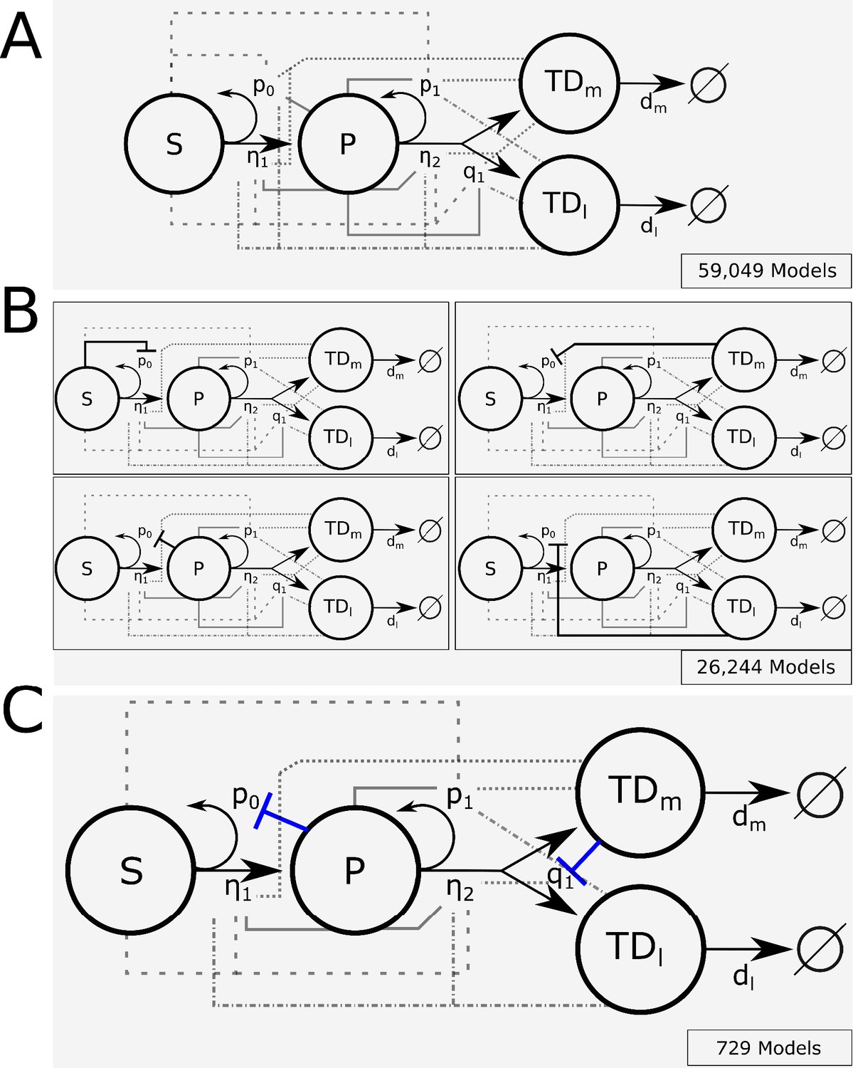
Branched lineage model of normal hematopoiesis with feedback regulation.
(A) Branched lineage model consisting of hematopoietic stem cells (HSC; S), multipotent progenitor cells (MPP; P), and postmitotic, terminally differentiated myeloid (TDm) and lymphoid (TDl) cells. Modulation of the HSC and MPP self-renewal fractions (p0 and p1), division rates (η1 and η2), and fate switching probability (q1) through feedback can arise from any cell type. The different line styles correspond to regulation by a particular cell type (dashed for S, solid for P, dot-dashed for TDl, and dotted for TDm). (B) Using Design Space Analysis, four candidate model classes are identified that differ in how HSCs are regulated. (C) Using biological data from the literature as discussed in the text, we reduced the model space by hypothesizing that factors secreted by terminally differentiated myeloid cells direct the fate of MPPs (e.g., IL-6) and those by MPPs suppress HSC self-renewal (e.g., CCL3).
Figure 2
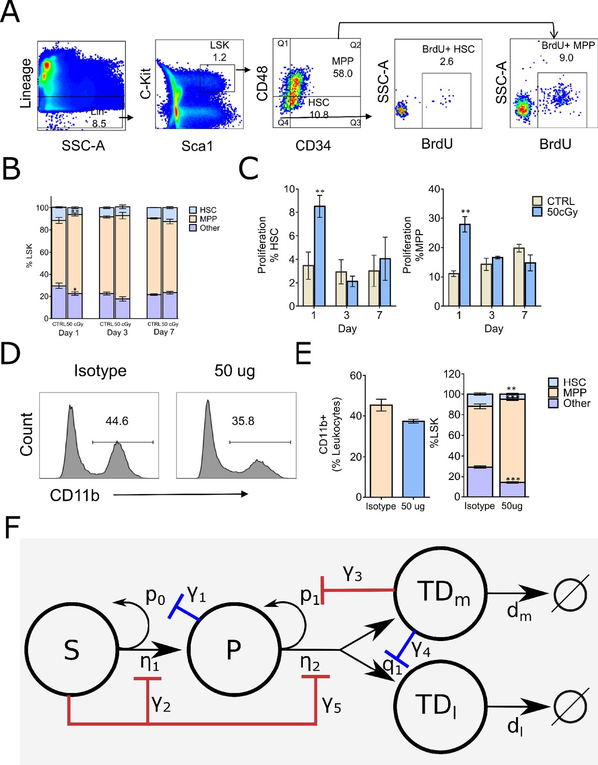
Fluorescence-activated cell sorting (FACS) analysis of mouse Lin–Sca-1+c-Kit+ (LSK) bone marrow stem/progenitor cells and the proposed branched lineage hematopoiesis model.
(A) Gating schema for phenotyping hematopoietic stem cells (HSC, defined as LSK CD34–CD48–) and multipotential progenitors (MPP, defined as LSK CD34+ CD48+), and BrdU incorporation in their respective compartments. (B) Distributions of HSC (blue), MPP (orange), and other (purple) compartments on days 1, 3, and 7 in the bone marrow (BM) of control (CTRL) B6 mice and mice that received 50 cGy radiation. (C) Frequency of HSC and MPP proliferation in CTRL (gray bars) and irradiated (blue bars) mice measured by BrdU incorporation on days 1, 3, and 7. Data are shown as mean ± SEM. *p<0.05. (D) Representative histograms depicting the frequency of myeloid cells as measured by CD11b expression in mice 24 hr after intravenous administration of isotype control (iso) or RB68C5 (50 μg) antibody. (E) Left panel: bar graph showing the frequency of CD11b+ cells in BM of mice that were treated with isotype control antibody (Iso; orange bar, n = 3 ) or RB68C5 antibody (50 μg; blue bars, n = 3). Right panel: HSC (blue), MPP (orange), and other cell type (purple) frequencies from mice that received isotype or RB6-8C5 antibody. Data are shown as mean ± SEM. *p<0.05. (F) Proposed feedforward-feedback model of hematopoiesis with associated feedback strengths denoted with γ1–γ5. The negative feedback loops shown in blue correspond to those suggested by previous experimental data (Reynaud et al., 2011; Staversky et al., 2018), while the negative feedback and feedforward loops in red are supported by our cell depletion experiments in (A–E).
Figure 3 with 2 supplements
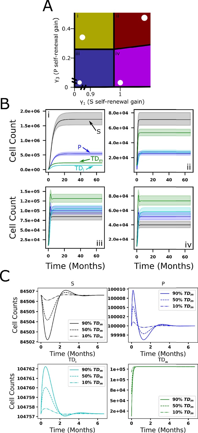
Qualitative behavior of feedforward-feedback model and parameter sensitivity.
(A) The colored regions (i–iv) represent areas of design space in which there are distinct qualitative behaviors as a function of the feedback gains γ1 and γ3 of the hematopoietic stem cell (HSC) and multipotential progenitor (MPP) self-renewal fractions, respectively. White dots denote specific parameter combinations. (B) The dynamics for each cell compartment within each of the four design space regions (i–iv). Solid lines represent ordinary differential equation (ODE) solutions using the specific parameter combinations (black dots in A) while the lightly colored regions represent the range of ODE solutions resulting from perturbations in γ1 and γ3 in a range within 0.9–1.1 times their original values. The blue and black curves correspond to the HSC and MPPs, respectively, the green and turquoise curves correspond to the myeloid and lymphoid cells. (C) The return to equilibrium following partial depletion of mature myeloid cells (10%, 50%, 90%) using the parameter combination (white dot) in region iii.
Figure 3—figure supplement 1
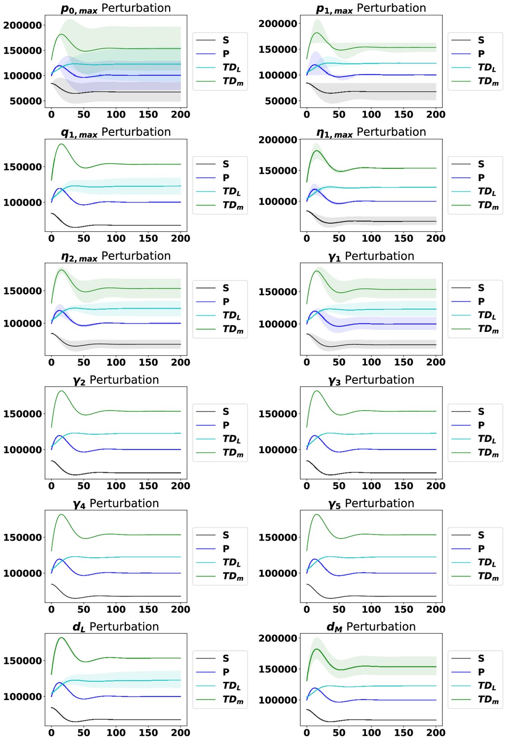
The dynamics from the steady state with perturbations of each parameter, as labeled, ranging from 90% to 110% of the original parameter value from Appendix 1—table 4.
The solid line represents the median of the perturbations, while the shaded region represents 95% of the perturbation dynamics.
Figure 3—figure supplement 2
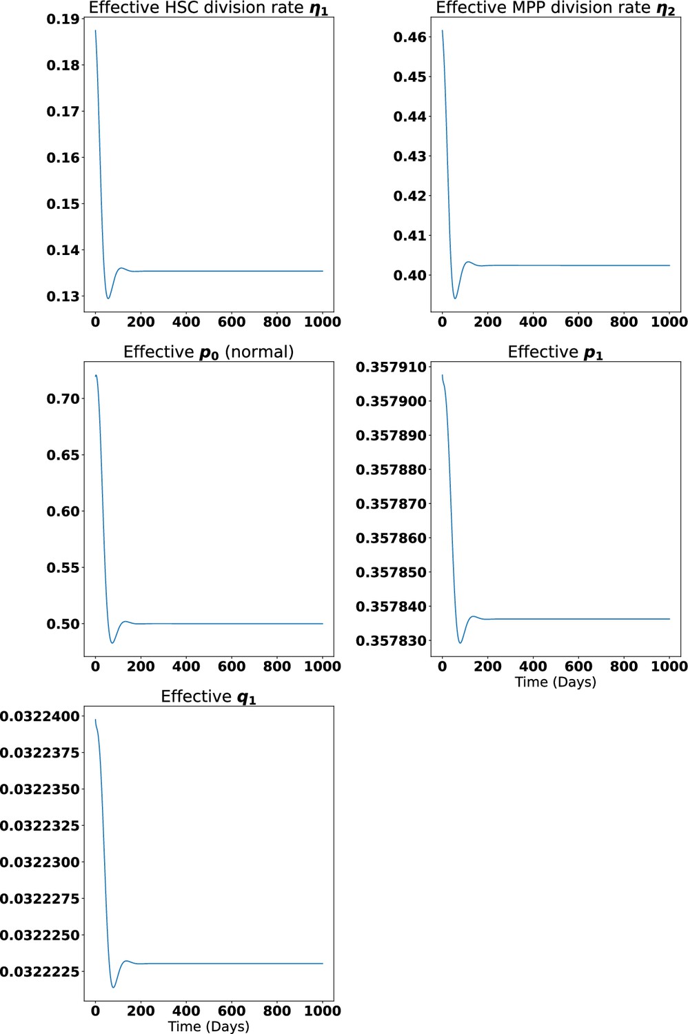
Effective parameters for proliferation, self-renewal, and branching as the solutions to the model for the normal hematopoietic system approach steady state.
Figure 4 with 6 supplements
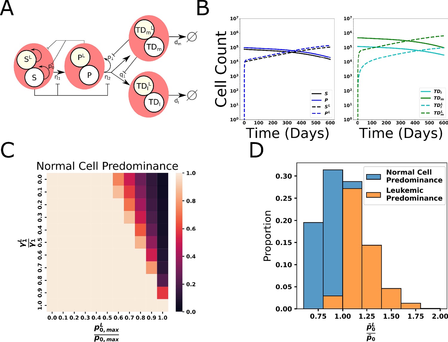
Extension of the model of hematopoiesis to chronic myeloid leukemia (CML).
(A) Schematic of two branched lineages consisting of normal and CML cell compartments. The two lineages share the same feedback architecture. The difference between the two lineages is the leukemic hematopoietic stem cell (HSC) self-renewal is less affected by negative feedback, denoted by p0L (see text). (B) Dynamics of hematopoiesis upon introduction of CML cells. We begin with having normal hematopoiesis at equilibrium. At time 0, 104 leukemic stem cells (HSCL, SL) cells are introduced to the system and subsequently expand over time at the expense of the normal cells, which decrease. (C) Sensitivity analyses of the outcomes of CML hematopoiesis with values corresponding to the proportion of parameter sets where less than 50% of terminal cells are leukemic. (D) The fitness of the leukemic stem cells relative to the normal stem cells, as measured by the ratio of their characteristic self-renewal fractions ( / ) determines whether CML will progress and leukemic cells will take over the system after CML stem cells are introduced.
Figure 4—figure supplement 1
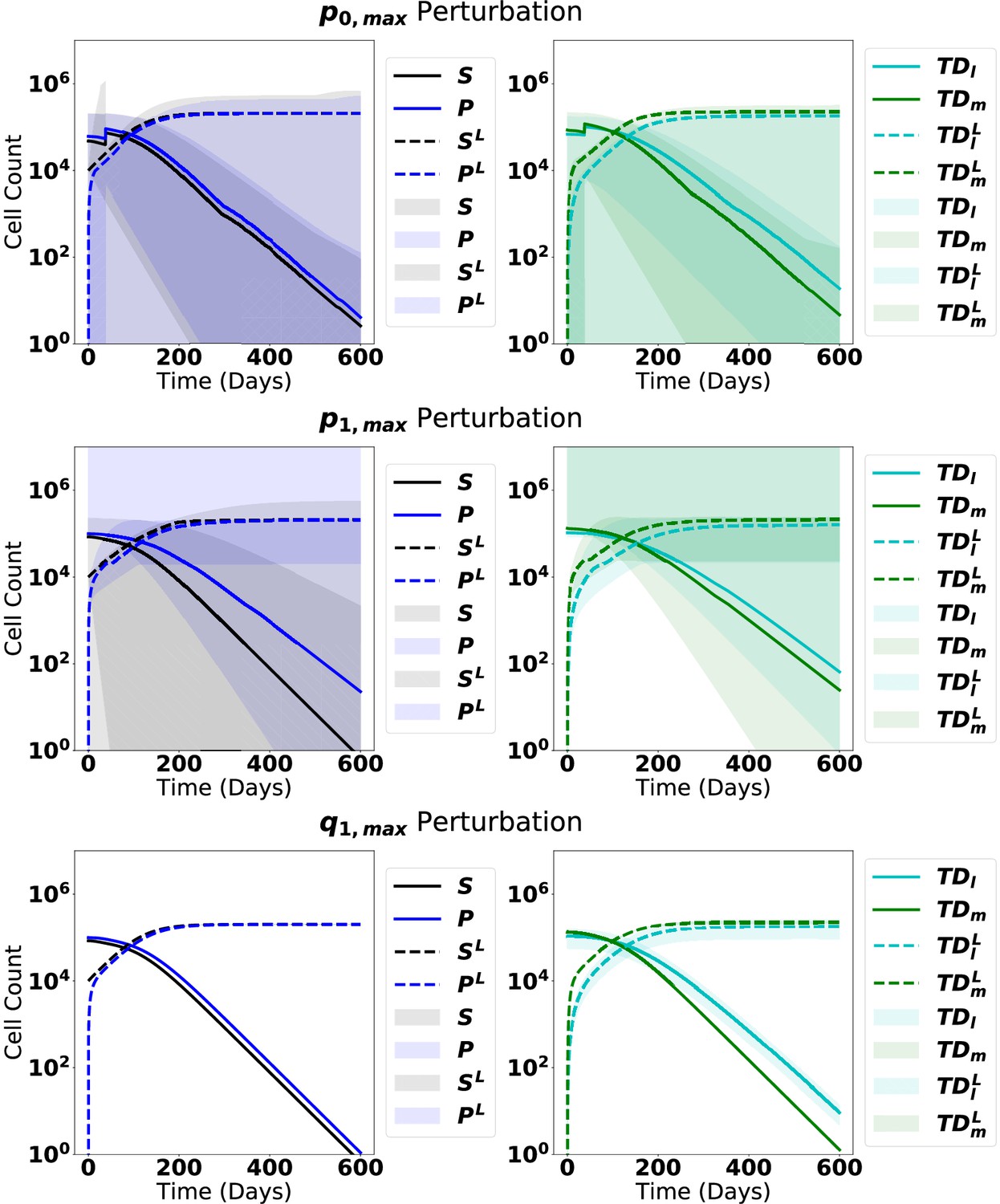
The dynamics from steady state upon introduction of leukemic stem cells with perturbations of each parameter, as labeled, ranging from 90% to 110% of the original parameter value in Appendix 1—table 5.
The solid line represents the median of the perturbations, while the shaded region represents 95% of the perturbation dynamics.
Figure 4—figure supplement 2
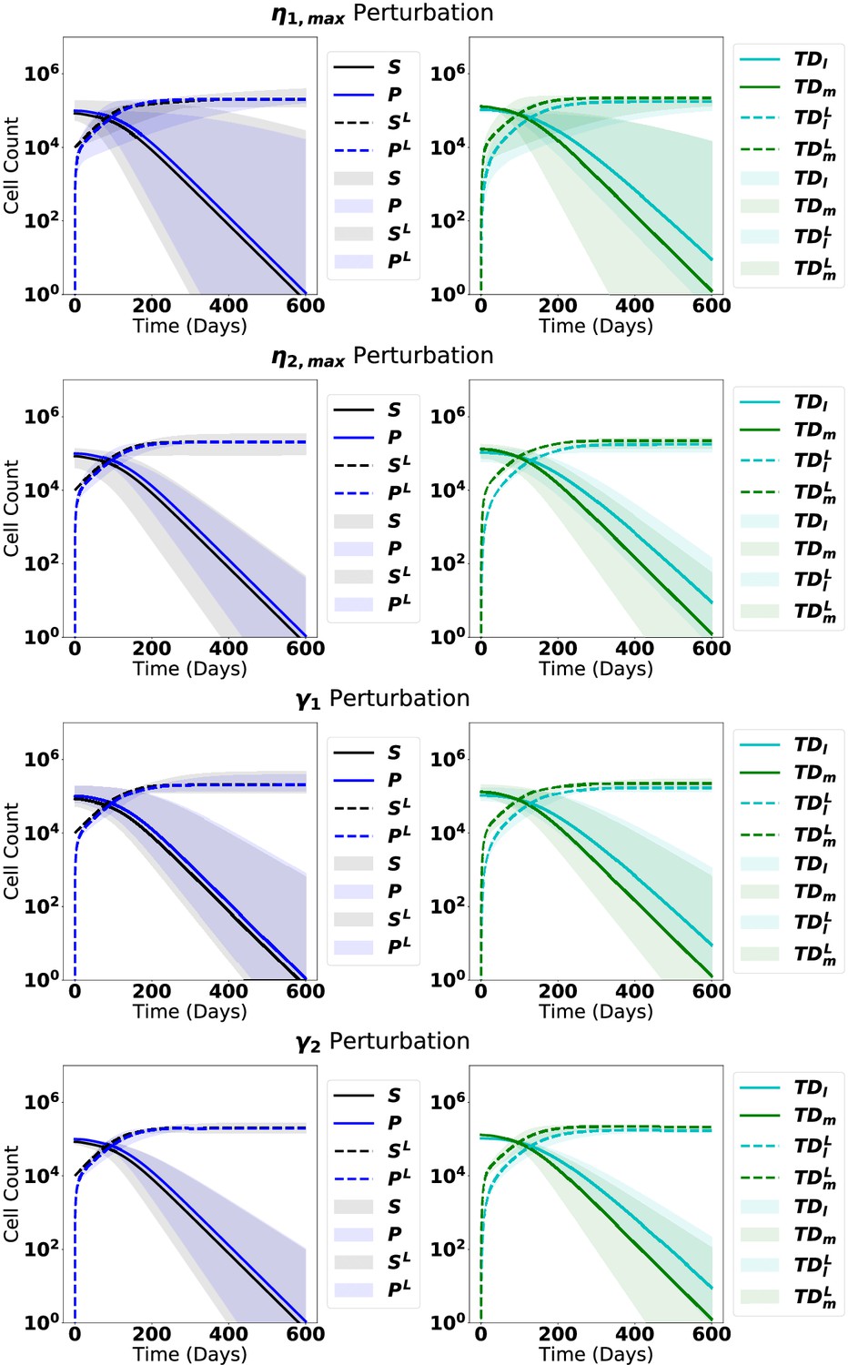
The dynamics from steady state upon introduction of leukemic stem cells with perturbations of each parameter, as labeled, ranging from 90% to 110% of the original parameter value in Appendix 1—table 5.
The solid line represents the median of the perturbations, while the shaded region represents 95% of the perturbation dynamics.
Figure 4—figure supplement 3
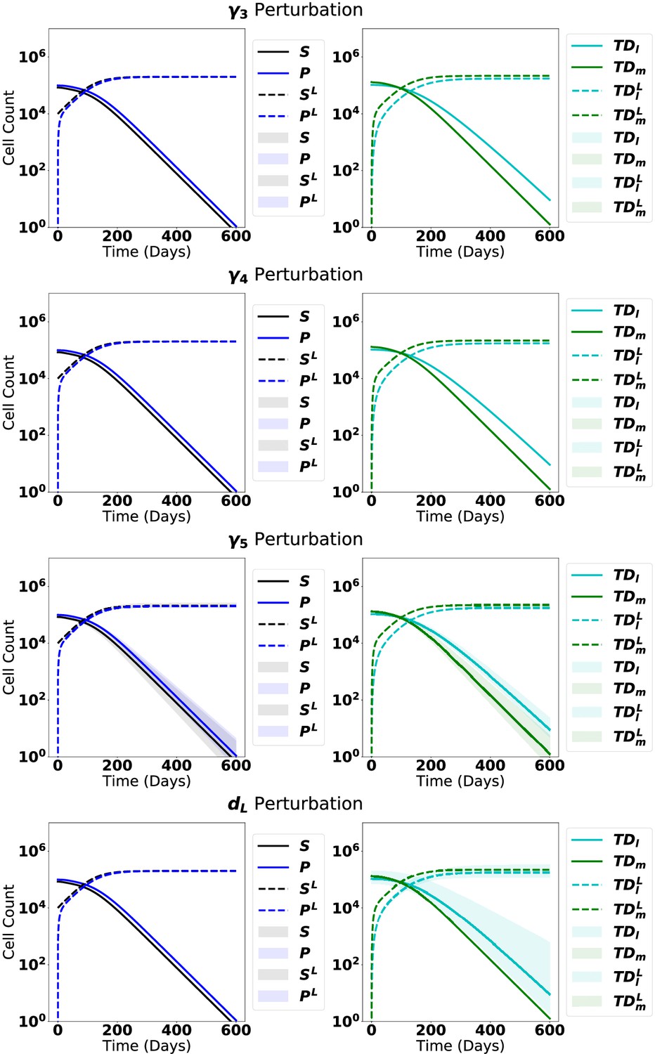
The dynamics from steady state upon introduction of leukemic stem cells with perturbations of each parameter, as labeled, ranging from 90% to 110% of the original parameter value in Appendix 1—table 5.
The solid line represents the median of the perturbations, while the shaded region represents 95% of the perturbation dynamics.
Figure 4—figure supplement 4
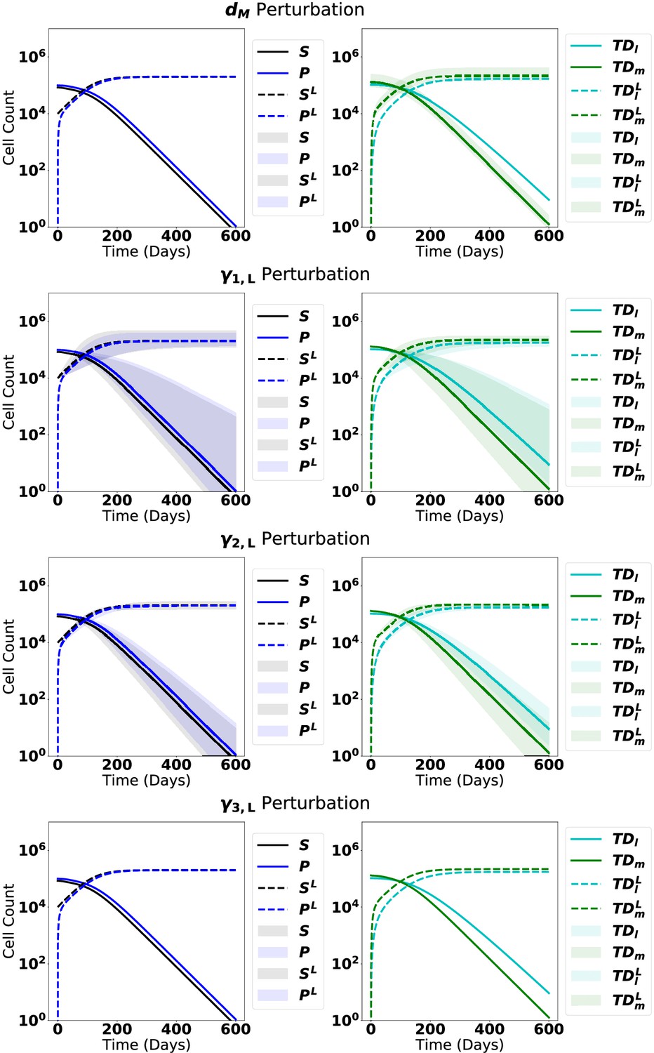
The dynamics from steady state upon introduction of leukemic stem cells with perturbations of each parameter, as labeled, ranging from 90% to 110% of the original parameter value in Appendix 1—table 5.
The solid line represents the median of the perturbations, while the shaded region represents 95% of the perturbation dynamics.
Figure 4—figure supplement 5
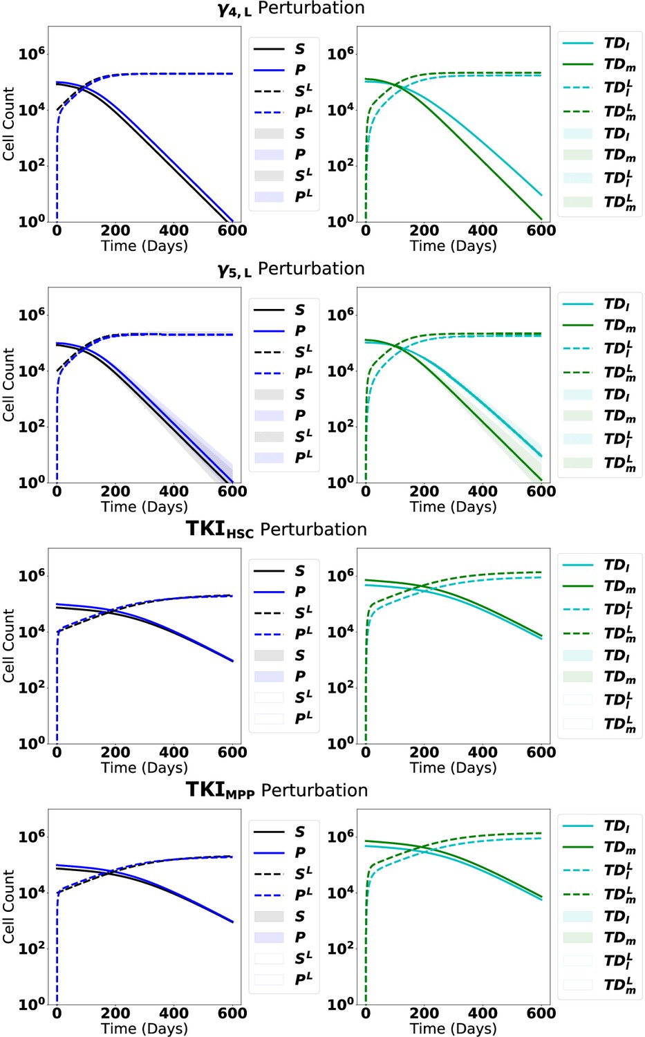
The dynamics from steady state upon introduction of leukemic stem cells with perturbations of each parameter, as labeled, ranging from 90% to 110% of the original parameter value in Appendix 1—table 5.
The solid line represents the median of the perturbations, while the shaded region represents 95% of the perturbation dynamics.
Figure 4—figure supplement 6
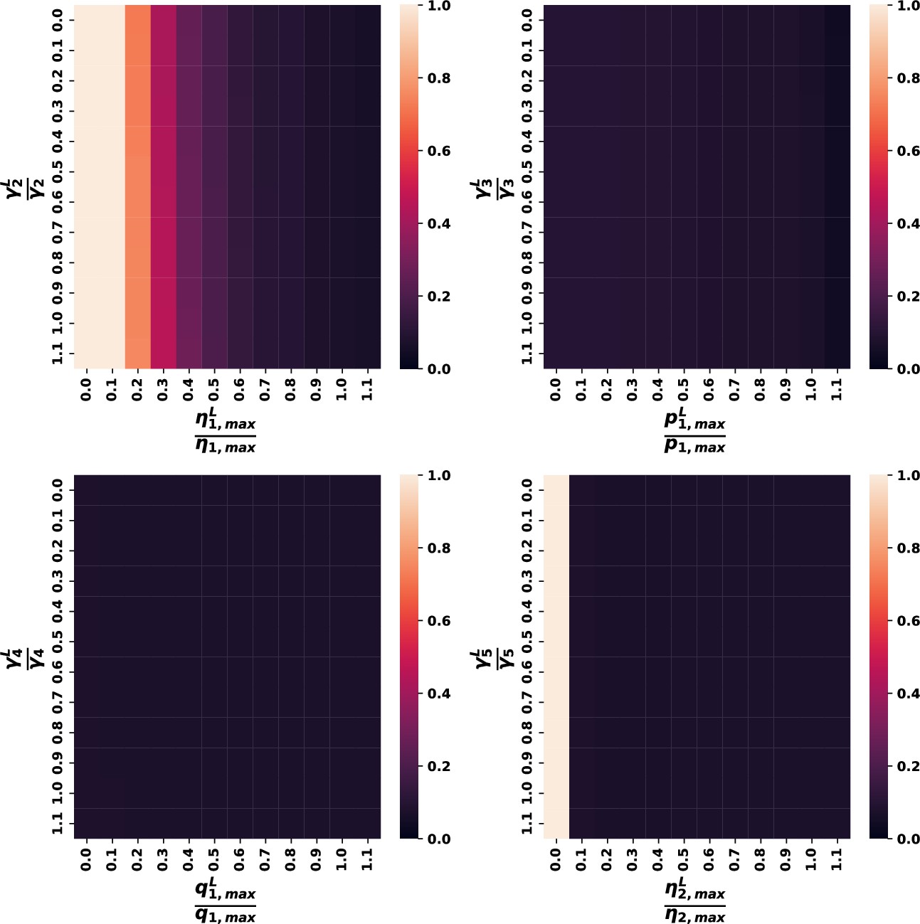
Variations in the other leukemic parameters and their associated gamma for all eligible parameter sets.
Plots display data using the same criteria as Figure 4C, but results show nearly complete insensitivity to changes in either value for the other leukemic parameters.
Figure 5 with 3 supplements
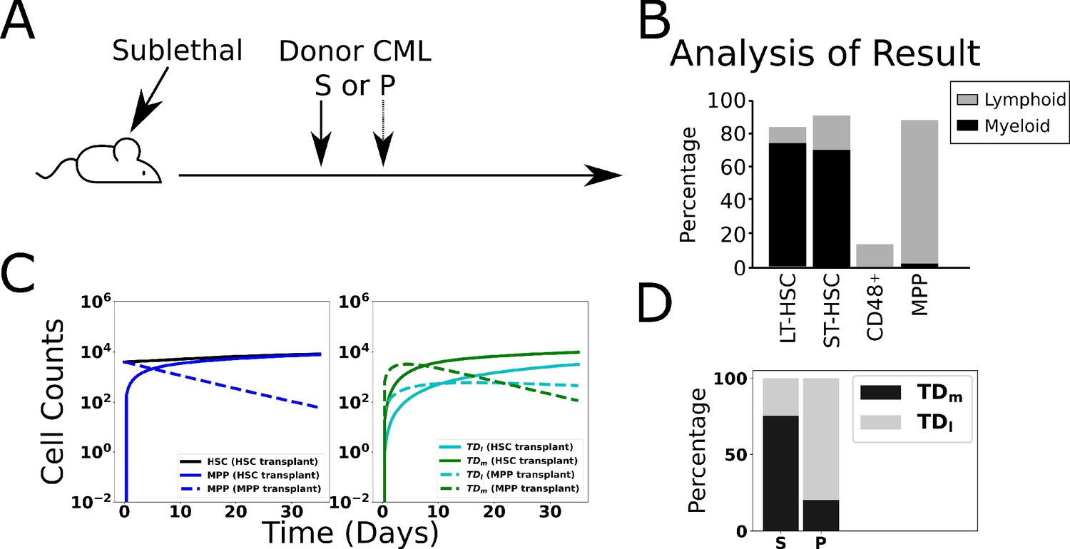
Validation of model through simulated transplant.
Results of a transplant experiment from Reynaud et al., 2011. Schematic (A) depicting the experimental pipeline and results (B), adapted from Figure 2A-C in Reynaud et al., 2011. When HSCL are transplanted into sublethally irradiated mice, chronic myeloid leukemia (CML)-like leukemia is induced and the myeloid cells expand. When leukemic multipotent progenitor cells (MPPL, PL) are transplanted, they do not stably engraft and transiently produce a larger fraction of differentiated lymphoid cells. (C) Simulated time evolutions of donor-derived HSCL, MPPL, and terminally differentiated lymphoid (TDl), and myeloid (TDm) cells when HSCL (solid) or MPPL (dashed) cells are transplanted. (D) Bar chart showing model predictions of the percentages of donor-derived myeloid and lymphoid cells after 35 d when HSCL or MPPL are transplanted, which is consistent with the experimental data in (B; see text).
Figure 5—figure supplement 1
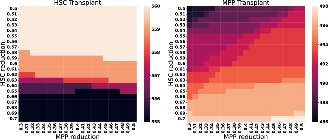
Heat map depicting the outcomes of transplant experiments in the presence of decrements of 50–70% HSCL and 30–50% MPPL from their equilibrium values (see text for details).
The heat map quantifies the number of parameter sets that are consistent with the experimental observations (Reynaud et al., 2011) that there is a simple majority of myeloid or lymphoid cells after 35 d when HSCL or MPPL are transplanted, respectively.
Figure 5—figure supplement 2
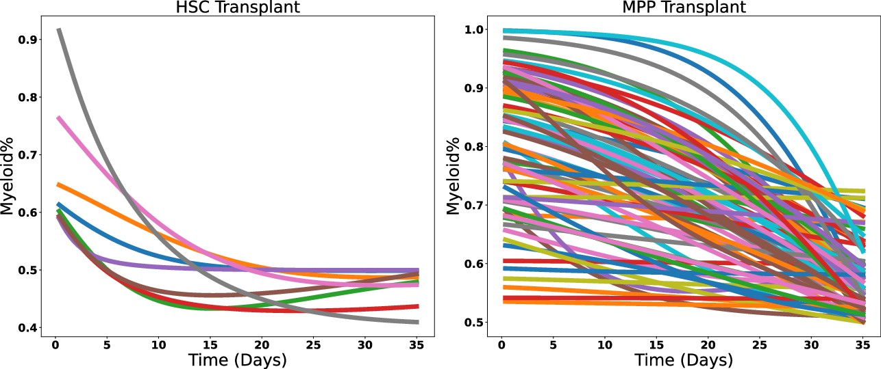
The dynamics of each parameter set that does not match the experimentally observed behavior of the transplant experiments from Reynaud et al., 2011.
These parameter sets are removed from the pool of eligible parameter sets if in the worst-case scenario for each parameter set they are not consistent with the criteria outlined in Figure 5—figure supplement 1.
Figure 5—figure supplement 3
Distributions of the remaining 478 parameters after removal determined through the depletion sweep.
Figure 6 with 4 supplements
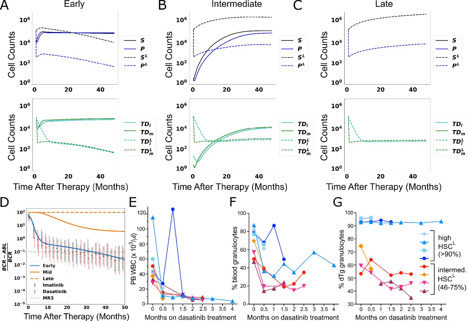
The response of chronic myeloid leukemia (CML) to tyrosine kinase inhibitor (TKI) therapy.
(A–C) Simulated cell dynamics of normal and leukemic cells in response to TKI therapy that is started at different time points in CML development (A, early times; B, intermediate times; C, late times). See text. (D) Simulated molecular response curves corresponding to the application of TKIs for each of simulations in (A–C). The simulated molecular response from (A) (blue) compares well with clinical data (symbols) measuring treatment responses to two different TKIs (imatinib, dasatinib) averaged across a cohort of patients (Glauche et al., 2018). The simulated molecular responses from (B) and (C) (orange solid and dashed curves) are indicative of primary resistance. (E–G) Experiments in chimeric mice (see text) that show that the size of the leukemic stem cell clone correlates with decreased response to TKI therapy. Peripheral blood (PB) leukocyte counts (E), percentage of PB granulocytes (F), and PB BCR-ABL1+ (leukemic) granulocyte chimerism (G) are shown in cohorts of mice treated with dasatinib. Blue symbols are chimeras bearing >90% BCR-ABL1+ HSCL, red-orange symbols are chimeras bearing 46–75% BCR-ABL1+ HSCL.
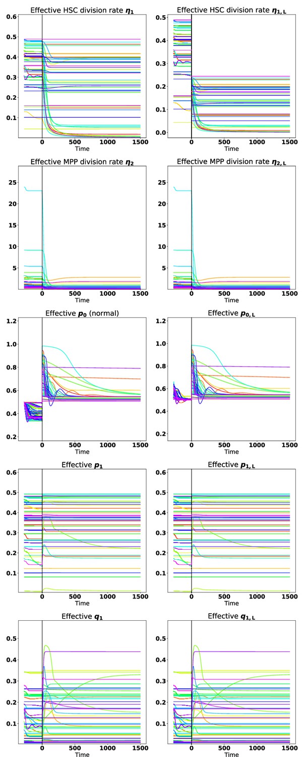
Figure 6—figure supplement 1
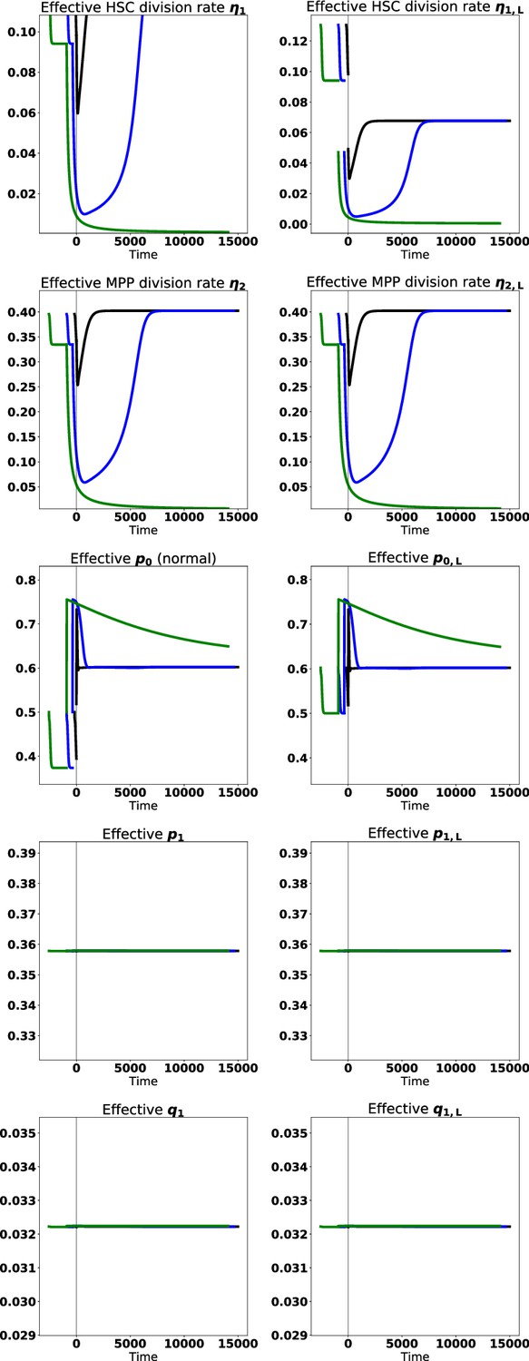
Effective parameters for proliferation, self-renewal, and branching after leukemic stem cells are added to the normal system at steady state, and after tyrosine kinase inhibitor (TKI) therapy begins for the cases shown in Figure 6 in the main text.
The vertical gray line depicts the start of treatment (time ). Black represents treatment at early times (shortly after chronic myeloid leukemia [CML] develops), blue denotes treatment at intermediate times, and green denotes treatment a long time after CML develops.
Figure 6—figure supplement 2
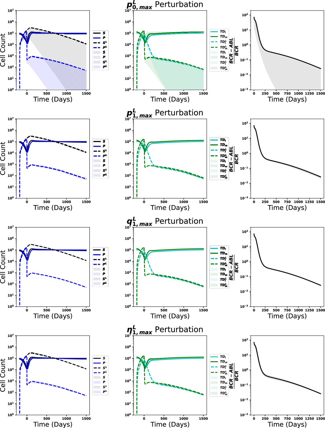
The dynamics from steady state upon introduction of leukemic stem cells with perturbations of each leukemic parameter, as labeled, ranging from 90% to 110% of the original parameter value (Appendix 1—table 4 for normal cells, Appendix 1—table 5 for leukemic cells), except for , which is never varied above the value.
The solid line represents the unperturbed state, while the shaded region represents the entire range of the perturbation dynamics.
Figure 6—figure supplement 3

The dynamics from steady state upon introduction of leukemic stem cells with perturbations of each leukemic parameter, as labeled, ranging from 90% to 110% of the original parameter value (Appendix 1—table 4 for normal cells, Appendix 1—table 5 for leukemic cells).
The solid line represents the unperturbed state, while the shaded region represents the entire range of the perturbation dynamics.
Figure 6—figure supplement 4
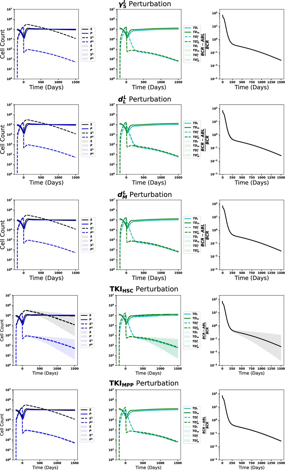
The dynamics from steady state upon introduction of leukemic stem cells with perturbations of each leukemic parameter, as labeled, ranging from 90% to 110% of the original parameter value (Appendix 1—table 4 for normal cells, Appendix 1—table 5 for leukemic cells).
The solid line represents the unperturbed state, while the shaded region represents the entire range of the perturbation dynamics.
Figure 7 with 2 supplements
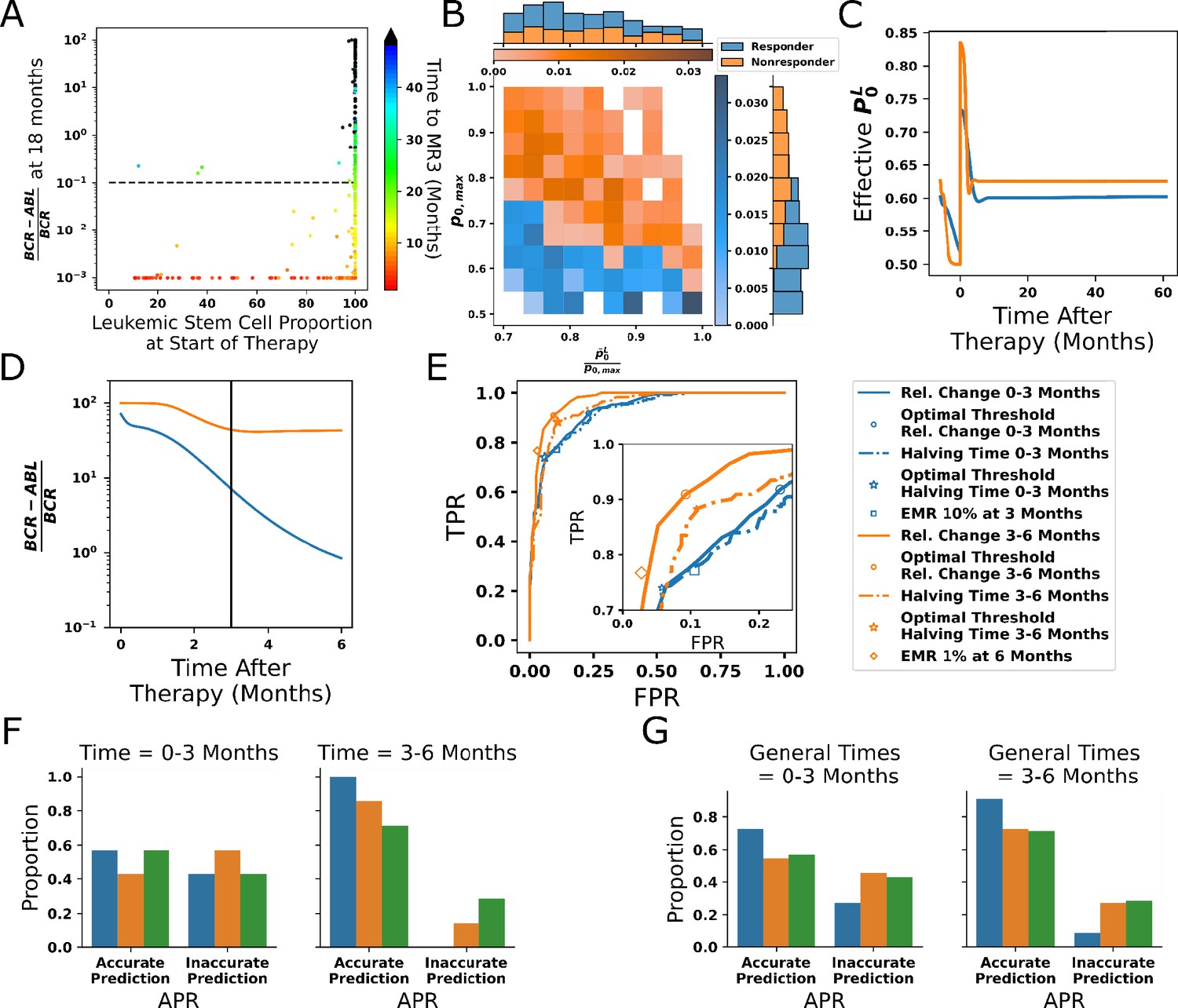
Leukemic stem cell load alone does not predict response to tyrosine kinase inhibitor (TKI) therapy.
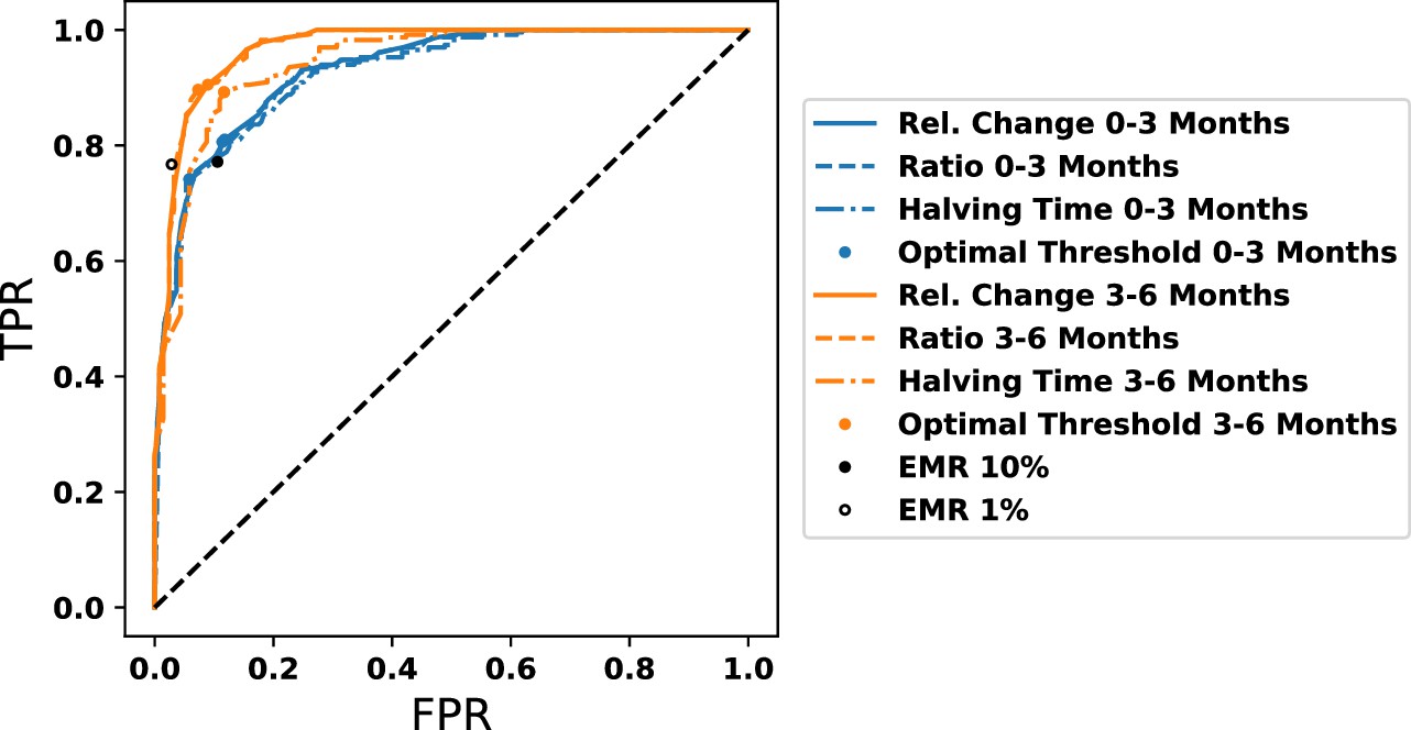
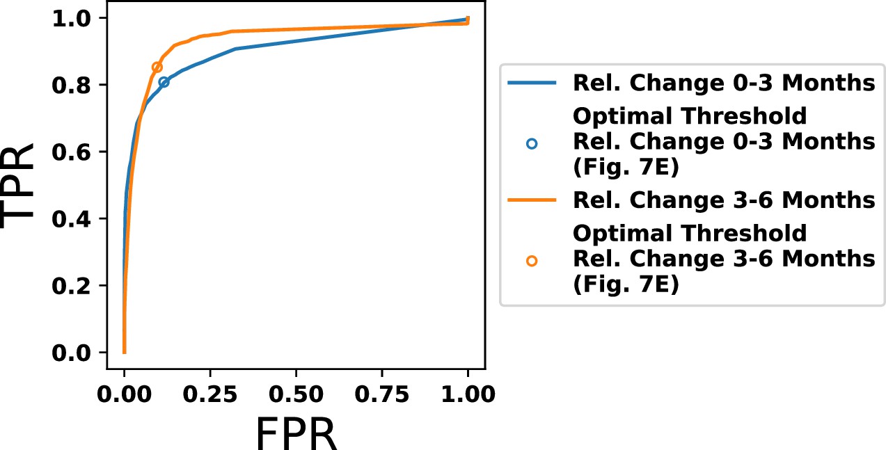
(A) Scatter plot of the distribution of simulated BCR-ABL1 transcripts at 18 mo after start of treatment as a function of the HSCL proportion at the start of TKI therapy for each of the 478 parameter sets. The time to reach MR3 (BCR-ABL1 transcripts less than 0.1%) is indicated by the color. (B) The proportion of parameter sets that achieve MR3 within 50 mo (responders, blue) and those that do not (nonresponders, orange) shown as a joint distribution of the parameters and using the minimum fitness threshold , which reveals the maximal self-renewal fraction of the normal HSC, (y-axis marginal distribution), distinguishes response across parameter combinations. (C) Dynamics of the effective leukemic stem cell self-renewal fraction for the parameter set used in Figure 6A–D (blue) and an arbitrary representative non-responsive parameter set (orange) during chronic myeloid leukemia (CML) development and before initiation of therapy (t < 0), and after application of TKI therapy (t > 0). (D) Early time dynamics (e.g., t = 0–3 mo; left of the vertical line) of the transcript levels reveal that it is difficult to distinguish responders (blue) from nonresponders (orange). At later times (e.g., t = 3–6 mo; right of the vertical line), the two populations are easier to distinguish. (E) Receiver operating curves (ROC) obtained from the 478 parameter sets using our new prognostic criterion based on the relative changes in transcript levels (solid) and the transcript halving time (dashed) for the first 3 mo (blue) and the second 3 mo (orange) after therapy. The prognostic thresholds (symbols) are identified by optimizing true and false positives rates. Early molecular response (EMR) at 3 mo (10% transcript levels) and 6 mo (1% transcript levels) are shown by the blue square and orange diamond, respectively. Inset: expanded view of the ‘elbow’ region of the ROC curves to display differences between the prognostic tests. Accuracy is improved using the 3–6 mo time window, and our new prognostic criterion outperforms the EMR and halving time prognostics in this time window. (F) The accuracy of the prognostic criteria applied to CML patient data (n = 7) treated using the same TKI dosing for the 6-month period after therapy is started. The results are consistent with the synthetic data in (E). (G) The prognostic criteria applied to patient data (n = 7) in which therapy could be changed but those changes were maintained for 6 mo (see text). Although the data are limited, the results are consistent with those in (E) and (F) suggesting increased accuracy using the 3–6-month window, and that the prognostic criterion based on relative change may yield more accurate predictions than EMR and halving time in the 3–6-month time frame.
Figure 7—figure supplement 1
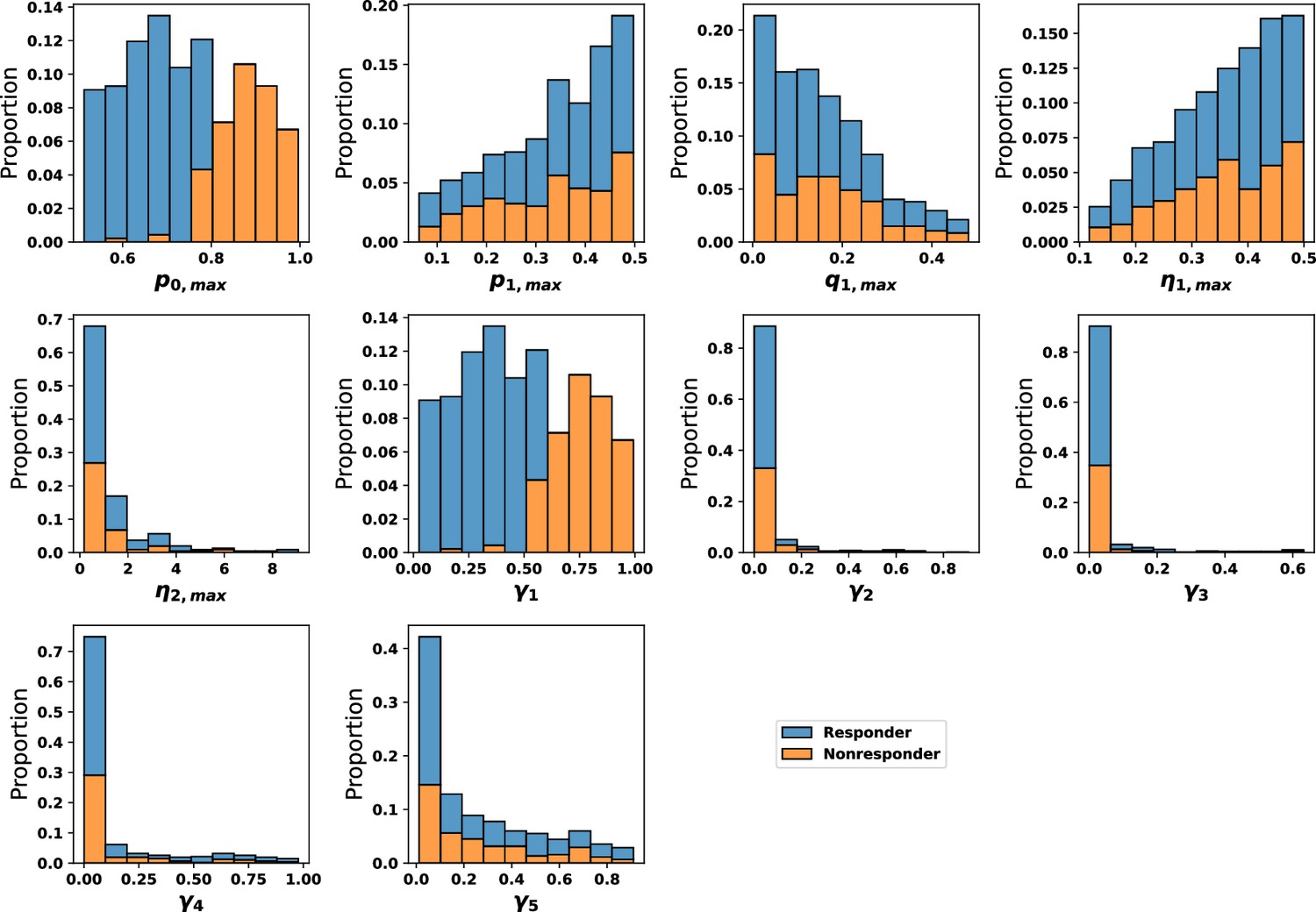
Parameter distributions by response to tyrosine kinase inhibitor (TKI) treatment using synthetic data.
Blue denotes a parameter set achieves MR3 within 50 mo (responder), and yellow denotes a parameter set that does not (non-responder).
Figure 7—figure supplement 2
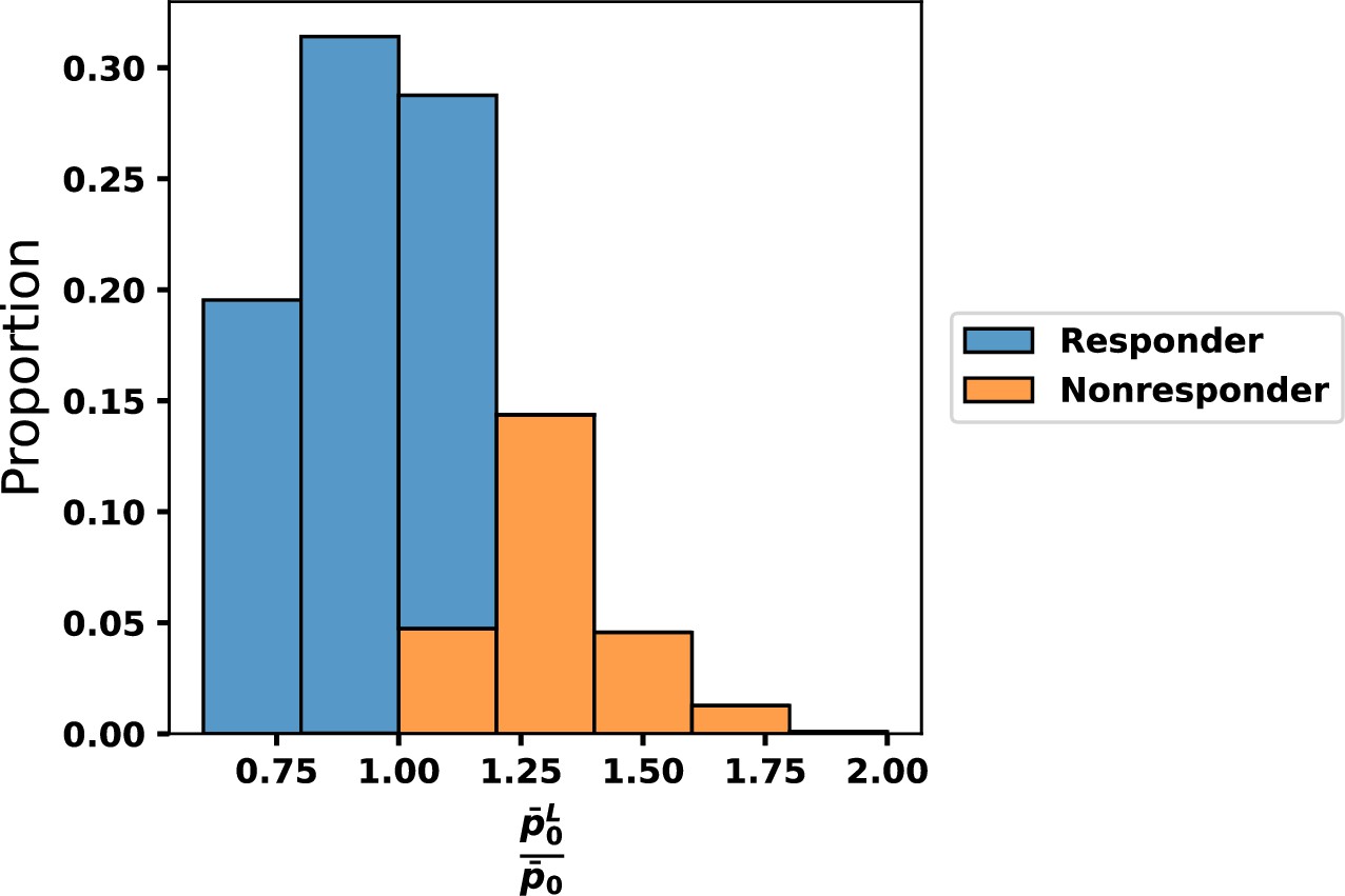
Comparison of the proportion of cases that successfully respond to therapy as a function of the ratio of characteristic values of leukemic and normal stem cells: .
The relative fitness is the critical determinant of whether chronic myeloid leukemia (CML) cells respond to tyrosine kinase inhibitor (TKI) treatment.
Figure 8 with 2 supplements
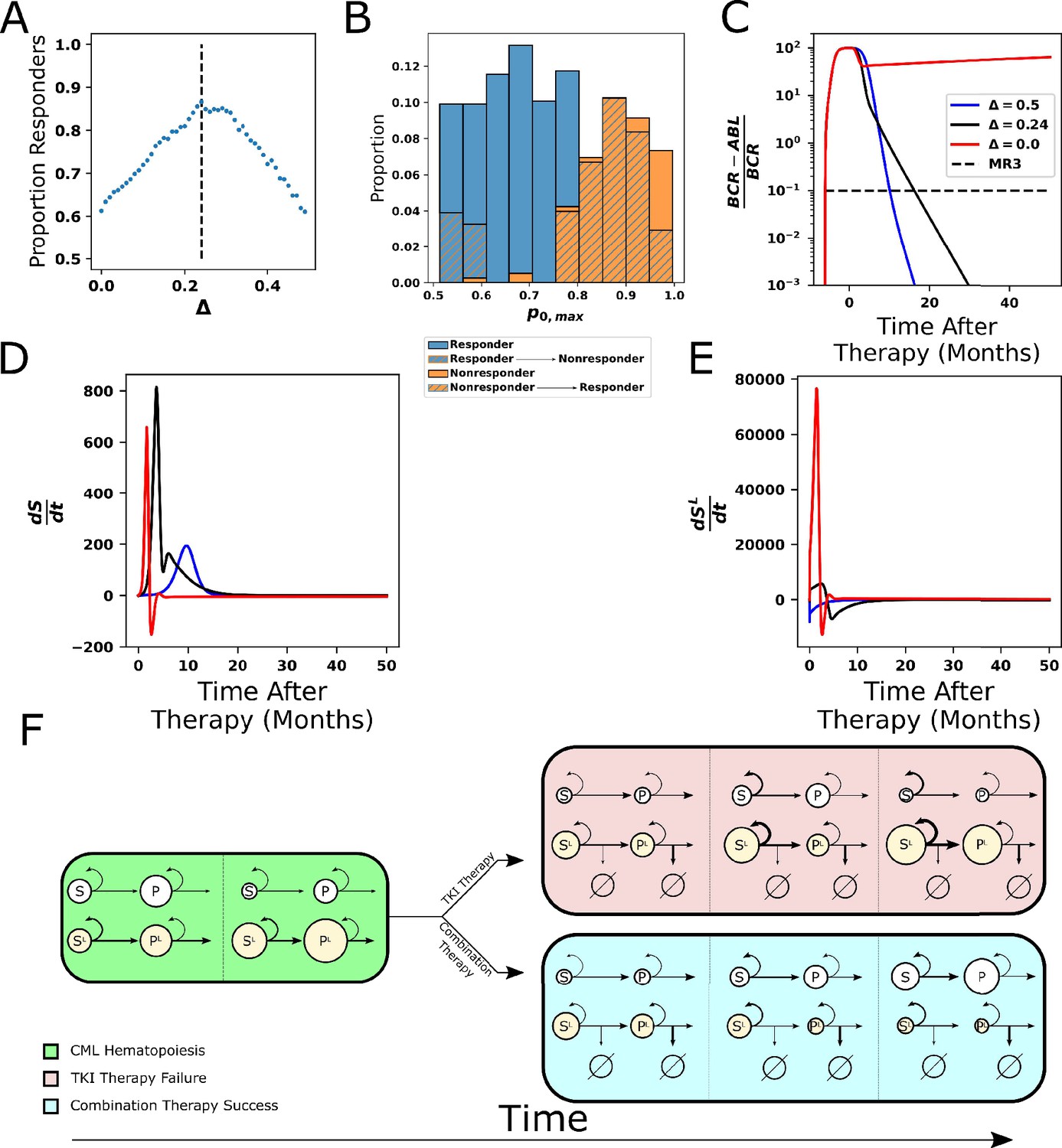
Combining tyrosine kinase inhibitor (TKI) therapy with differentiation promoters enhances response to treatment.
(A) The proportion of the 478 parameter sets that achieve MR3 under combined TKI and differentiation therapy depends nonmonotonically on the strength Δ of the differentiation therapy, with the peak response (86.8%) occurring at Δ = 0.24. (B) The maximum stem cell self-renewal fraction for a single in Figure 7B (marginal y) with hatching indicating the effects of the combination of TKI and differentiation therapy with Δ = 0.24. Blue hatching indicates nonresponders (who did not achieve MR3) that become responders (achieve MR3) while orange hatching indicates responders that become nonresponders upon combined treatment. Differentiation promoters allow nonresponders to TKI therapy with large self-renewal fractions to reach MR3. The opposite outcome, loss of MR3 in a TKI responder, primarily occurs only at the smallest self-renewal fractions. (C) Time evolution of BCR-ABL1 transcripts during combination therapy, with Δ = 0.24 (black) and Δ = 0.5 (blue), using the parameter set from Figure 5B that does not achieve MR3 using TKI monotherapy (red). (D, E) The time derivatives of the number of normal (D) and leukemic (E) stem cells during combination therapy. The differentiation promoter attenuates the rapid increases in the rates of change at early times after therapy starts in both normal and leukemic cells, but the attenuation is much larger in the leukemic cells. This results in the growth of normal cells, while leukemic cells experience restricted growth or outright depletion depending upon the differentiation therapy strength. (F) Simplified diagram representing the key interactions between the cells and the impact on outcomes of TKI and combination therapy. Green: chronic myeloid leukemia (CML) hematopoiesis depicting the loss of normal stem cells and progenitors and the increase in leukemic stem cells and progenitors. Red fill: TKI treatment failure. The TKI-induced death of leukemic progenitors relieves negative feedback and increases stem cell self-renewal, resulting in increases in both normal and leukemic stem cells, and eventually their progeny (panel 2). The increases are larger for the leukemic cells because their self-renewal fraction is bigger. Increases in the leukemic progenitor compartment (panel 3) drive down the self-renewal fraction of normal stem cells proportionally more than for the leukemic stem cells. The increases in HSCL also drive down proliferation rates, which makes the leukemic cells less responsive to TKI treatment. Altogether, this makes the leukemic cells more fit than the normal cells and results in therapy failure. Blue fill: treatment by combined TKI and pro-differentiation therapy reduces stem cell self-renewal relative to TKI monotherapies, equalizes the normal and leukemic self-renewal fractions, which limits leukemic stem cell growth and limits decreases in proliferation rates, making the HSCL and MPPL more susceptible to TKI-induced death (panel 2). This allows repopulation of the bone marrow by normal stem cells and progenitors to occur (panel 3).
Figure 8—figure supplement 1

Changes in the parameter distributions from Figure 7—figure supplement 1 when combined differentiation and tyrosine kinase inhibitor (TKI) therapy is administered.
Blue denotes a parameter set achieves MR3 within 50 mo, and orange denotes parameter sets that do not. Orange hatching denotes a parameter set that achieves MR3 within 50 mo with TKI monotherapy, but does not achieve MR3 within 50 mo under combination therapy. Blue hatching denotes a parameter set that does achieve MR3 within 50 mo with combination therapy but does not with TKI therapy alone.
Figure 8—figure supplement 2

Variations in and for all parameter sets with combination therapy show improvement of response with combination therapy compared to Appendix 1—figure 11 (bottom right).
Plots display data using the same criteria as Appendix 1—figure 11 (bottom right).
Appendix 1—figure 1
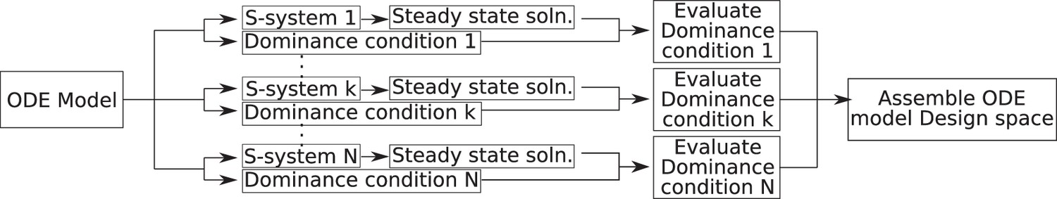
Flow chart for design space analysis (DSA).
Given an ordinary differential equation (ODE), we can obtain the design space by obtaining all S-systems, steady states, and evaluated dominance conditions. S-systems that do not satisfy the dominance condition are not included in the design space.
Appendix 1—figure 2
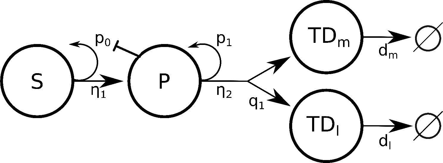
Lineage schematic depicting a stem cell and terminally differentiated cell with negative feedback onto stem cell self-renewal probability .
Appendix 1—figure 3
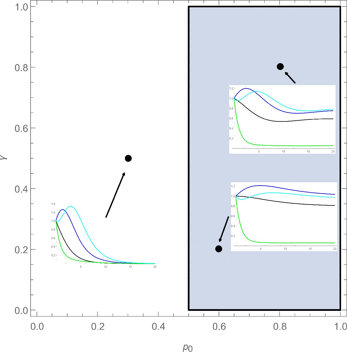
Design space for four-cell lineage model.
The design space is showing a slice of parameter space varying the max self-renewal probability () and feedback gain for stem cells (). If we are to sample parameters sets (shown by points), we observe oscillatory behavior in the full system, as shown by the time evolution plots.
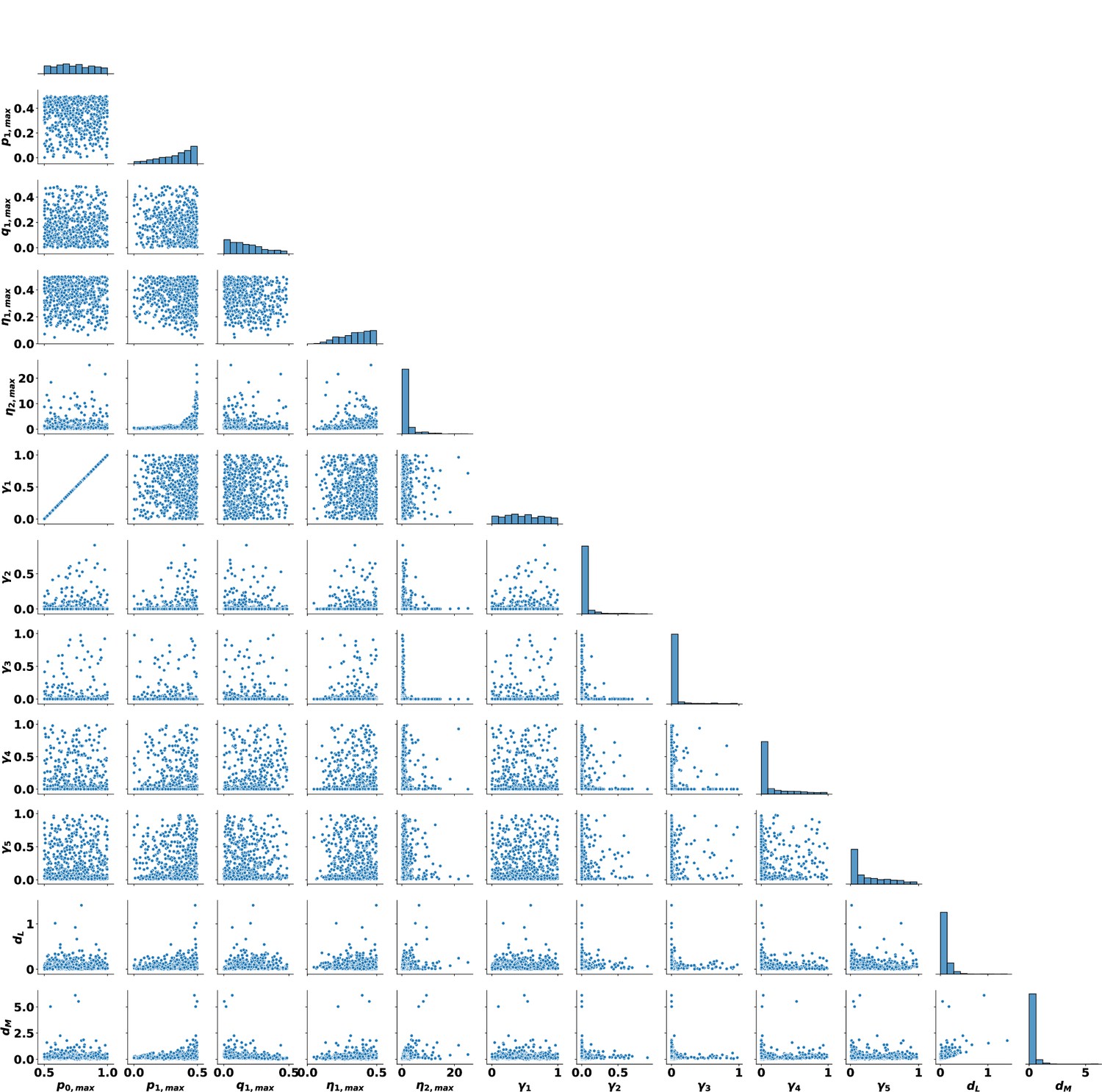
Appendix 1—figure 4
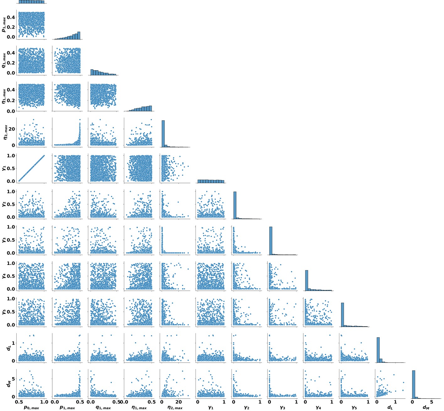
Pairwise parameter distributions for all 1493 parameter sets found from the gridsearch.
The overall distributions for each parameter are shown along the diagonal.
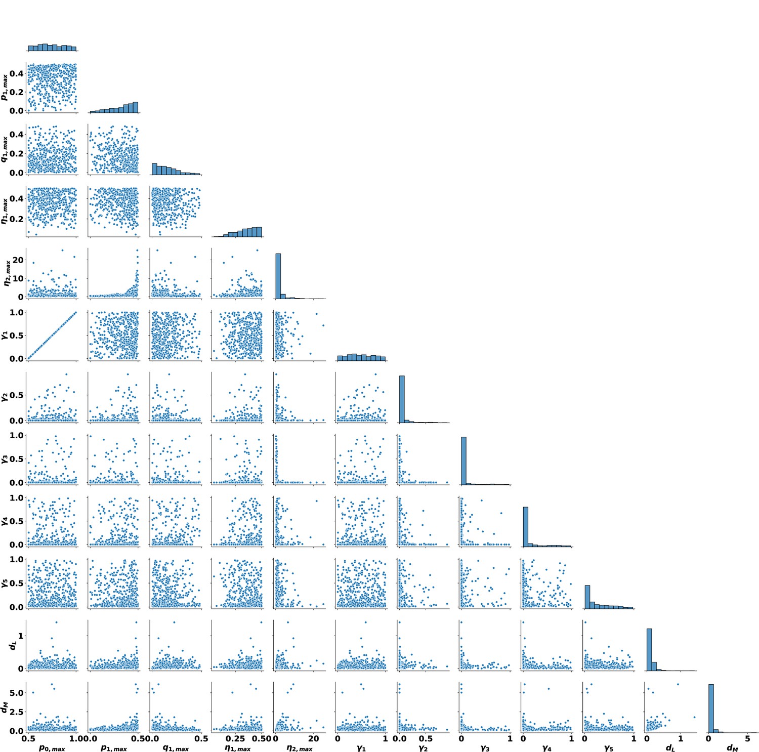
Appendix 1—figure 5
Pairwise parameter distributions for the 563 parameter sets from Appendix 1—figure 4 that have feedforward gain .
The overall distributions for each parameter are shown along the diagonal.
Appendix 1—figure 6
A spaghetti plot showing the dynamics of the effective proliferation, self-renewal, and branching parameters for 50 parameter sets under tyrosine kinase inhibitor (TKI) treatment started at early times.
Appendix 1—figure 7
Comparison between our prognostic and alternate prognostics, as labeled, at the first and second 3 mo after the start of therapy.
Appendix 1—figure 8
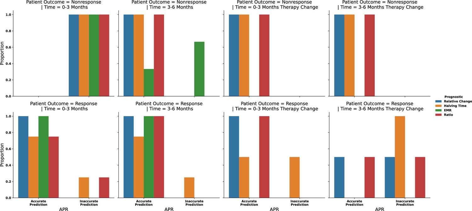
The ability of prognostic criteria to predict MR3 by 18 mo is evaluated using anonymized patient data (n = 11) in which patients received the same therapy for 6 mo either from the start of therapy or after a change in therapy.
The first two columns correspond to results when the same therapy is applied for 6 mo after patient diagnoses. The last two columns correspond to patients who have had a change of therapy, but the new therapy is maintained for 6 mo. The Early molecular response (EMR) prognostic criterion is not used when the patients have had a therapy change.
Appendix 1—figure 9
The predictive ability of each prognostic criterion from Appendix 1—figure 8 but grouped based upon patient (n = 11) outcome (blue, responder; and yellow, nonresponder) and the time frame for prediction.
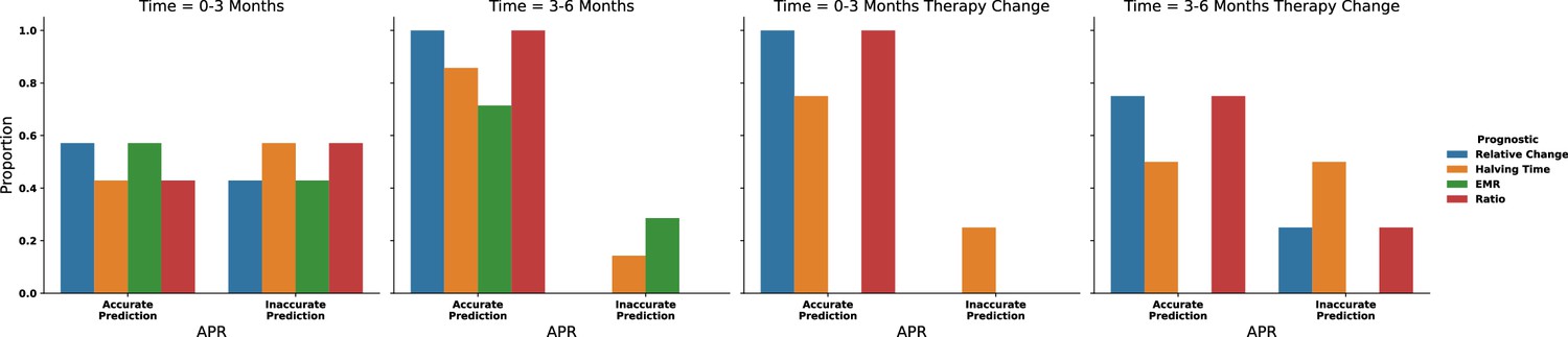
Appendix 1—figure 10
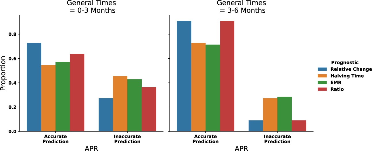
Aggregating the accuracy of prognostic criteria predictions with patient data (n = 11) from Appendix 1—figure 8 where a general time of 0–3 mo contains both 0–3 mo after start of therapy and after therapy change.
The 3–6-month data is aggregated similarly.
Appendix 1—figure 11
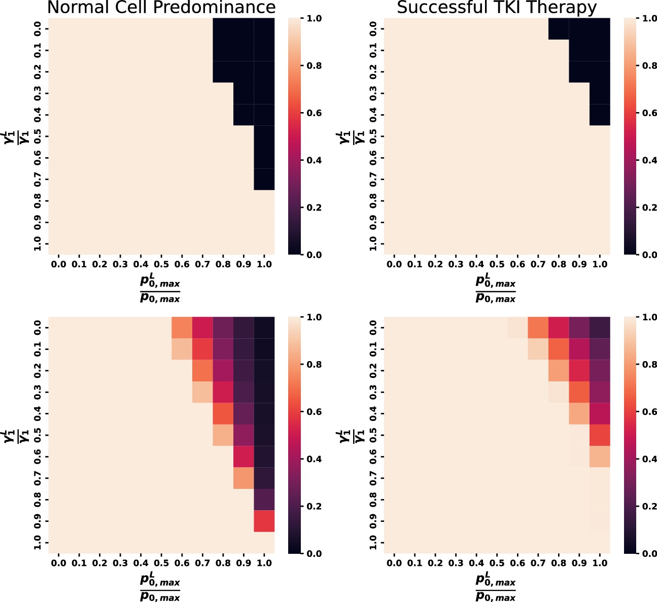
Variations in and for the individual parameter set from Figure 6 (top) and all eligible parameter sets (bottom).
Left heat maps display the proportion of parameter sets that maintain dominance of normal cells in the system in the lighter regions and the proportion that possess leukemic cell dominance in the darker regions. The right heat maps indicate proportion of cases where parameter sets achieve MR3 within 50 mo with lighter values associated with a higher proportion of response. Biologically relevant parameter combinations exist within darker regions on the bottom left and regions within orange to purple on the bottom-right plot.
Appendix 1—figure 12
Combinations of leukemic values with similar overall response rates to tyrosine kinase inhibitor (TKI) therapy (see text) yield similar distributions of response.
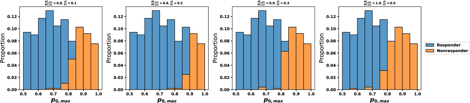
Appendix 1—figure 13
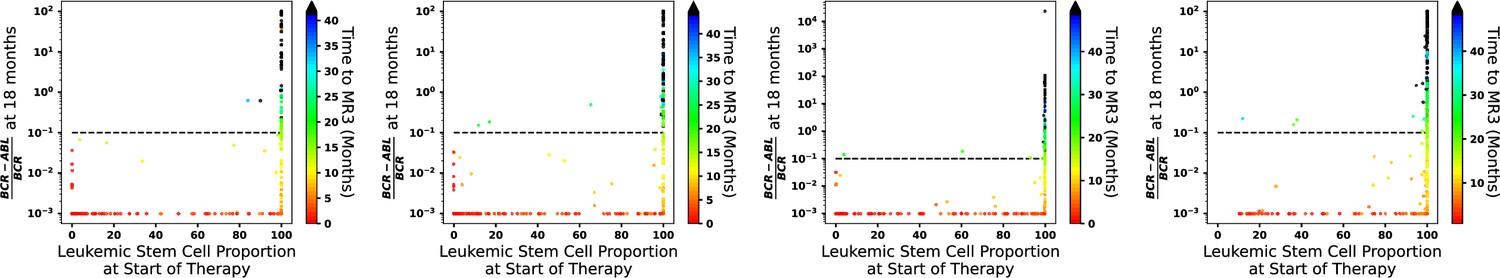
Simulated distributions of response to tyrosine kinase inhibitor (TKI) therapy as a function of initial proportion of leukemic stem cells is qualitatively similar across the parameter combinations from Appendix 1—figure 12 (from left to right): and , and , and , and and .
Appendix 1—figure 14
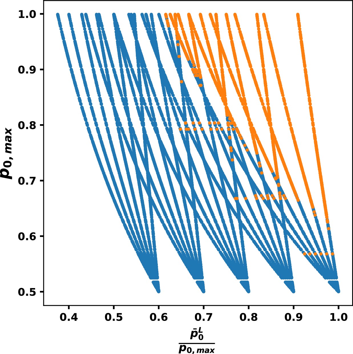
Comparison of trajectories of response as functions of and .
For each value of , there is one tree starting from , then for each up to the tree splits into six branches. Dot color denotes whether a parameter set responds (blue) or does not respond (orange).
Appendix 1—figure 15
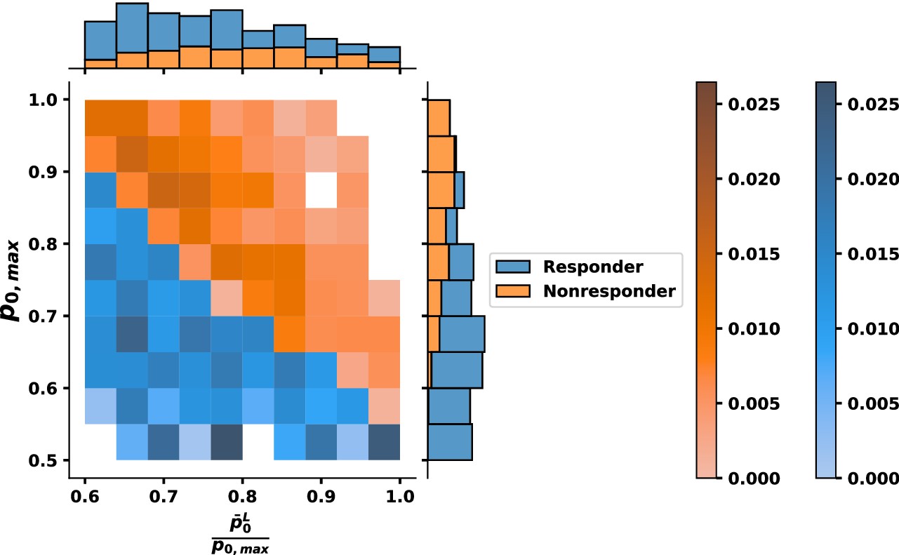
Bivariate histogram for response to tyrosine kinase inhibitor (TKI) therapy where the relative fitness of is .
Individual variable marginal distributions are shown along the sub-axes.
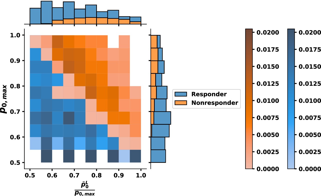
Appendix 1—figure 16
Bivariate histogram for response to tyrosine kinase inhibitor (TKI) therapy where the relative fitness of is .
Individual variable marginal distributions are shown along the sub-axes.
Appendix 1—figure 17
Prognostic value sweep applied to combinations of and with leukemic predominance > 60%.
Optimal values from Figure 7E are no longer the optimal across all combinations, but the 3–6-month time frame still outcompetes 0–3-month time frame.
Tables
Appendix 1—table 1
A sample of S-systems from Equations 14–18.
| S-system 1 | S-system 2 | S-system 3 | S-system 4 | |
|---|---|---|---|---|
| 0 | ||||
| Boundary 1 | ||||
| Boundary 2 |
Appendix 1—table 2
Parameter values used to model the normal hematopoietic system.
| Parameter | Description |
|---|---|
| Maximal self-renewal fraction of HSC | |
| Maximal self-renewal fraction of MPP | |
| Maximum branching fraction from MPP to | |
| Maximum HSC proliferation rate | |
| Maximum MPP proliferation rate | |
| Feedback gain on HSC self-renewal fraction | |
| Feedback gain on HSC proliferation rate (from HSC) | |
| Feedback gain on MPP self-renewal fraction | |
| Feedback gain on MPP branching fraction | |
| Feedforward gain on MPP proliferation rate | |
| Death rate of | |
| Death rate of |
-
HSC: hematopoietic stem cell; MPP: multipotential progenitor.
Appendix 1—table 3
Additional parameter values used to model the chronic myeloid leukemia (CML) cell population dynamics and effect of tyrosine kinase inhibitor (TKI) therapy.
| Parameter | Description |
|---|---|
| Maximal self-renewal fraction of HSC | |
| Maximal self-renewal fraction of MPP | |
| Maximum branching fraction from MPP to | |
| Maximum HSC proliferation rate | |
| Maximum MPP proliferation rate | |
| Feedback gain on HSC self-renewal fraction | |
| Feedback gain on HSC proliferation rate (from HSC ) | |
| Feedback gain on MPP self-renewal fraction | |
| Feedback gain on MPP branching fraction | |
| Feedforward gain on MPP proliferation rate | |
| Death rate of | |
| Death rate of | |
| Death rate of HSC due to TKI therapy | |
| Death rate of MPP due to TKI therapy |
-
HSC: hematopoietic stem cell; MPP: multipotential progenitor.
Appendix 1—table 4
Appendix 1—table 5
Additional parameter values used to model the chronic myeloid leukemia (CML) cell population dynamics in Figures 4A ,B—7 in the main text.
| Parameter | Value |
|---|---|
| 0.756641 | |
| 0.357913 | |
| 0.032241 | |
| 0.197639 | |
| 0.47088 | |
| 0.2566405 | |
| 0.197639 | |
| 0.47088 | |
| 0.2566405 | |
| 0.543987 | |
| 0.000165 | |
| 0.000428 | |
| 0.201311 | |
| 0.024757 |
Appendix 1—table 6
Secondary parameter values used as a representative case to model nonresponsive chronic myeloid leukemia (CML) cell population dynamics in Figures 7C, D, 8 in the main text.
| Parameter | Value |
|---|---|
| 0.838481 | |
| 0.009776 | |
| 0.418627 | |
| 0.226025 | |
| 0.247591 | |
| 0.676962 | |
| 0.000219 | |
| 0.000326 | |
| 0.367564 | |
| 0.168132 | |
| 0.071273 | |
| 0.155649 | |
| 0.838481 | |
| 0.009776 | |
| 0.418627 | |
| 0.226025 | |
| 0.247591 | |
| 0.338481 | |
| 0.000219 | |
| 0.000326 | |
| 0.367564 | |
| 0.168132 | |
| 0.071273 | |
| 0.155649 | |
| 0.25 | |
| 30 |
Additional files
Download links
A two-part list of links to download the article, or parts of the article, in various formats.
Downloads (link to download the article as PDF)
Open citations (links to open the citations from this article in various online reference manager services)
Cite this article (links to download the citations from this article in formats compatible with various reference manager tools)
Predictive nonlinear modeling of malignant myelopoiesis and tyrosine kinase inhibitor therapy
eLife 12:e84149.
https://doi.org/10.7554/eLife.84149


