Kinetochore-fiber lengths are maintained locally but coordinated globally by poles in the mammalian spindle
- Tetrad Graduate Program, University of California, San Francisco, United States
- Department of Bioengineering & Therapeutic Sciences, University of California, San Francisco, United States
- Developmental & Stem Cell Biology Graduate Program, University of California, San Francisco, United States
- Biochemistry & Biophysics Deptartment, University of California, San Francisco, United States
- Chan Zuckerberg Biohub, United States
Figures
Figure 1 with 9 supplements
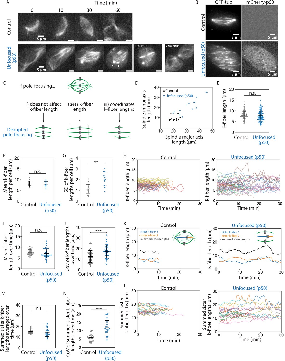
Spindle poles coordinate but do not maintain kinetochore-fiber lengths.
See also Figure 1—videos 1–3. (A) Representative confocal timelapse images of spindle assembly showing max-intensity z-projections of HaloTag-β-tubulin PtK2 spindles labeled with JF 646, from nuclear envelope breakdown at t = 0 through cytokinesis. mCherry-p50 was infected into unfocused but not control cells. Arrowheads mark where both centrosomes were observed to be disconnected from the spindle. (B) Max-intensity z-projections of representative confocal images of PtK2 spindles with GFP-α-tubulin (control and unfocused) and mCherry-p50 (unfocused only). (C) Cartoon model of a mammalian spindle with chromosomes (gray) and microtubules (green), with predictions for k-fiber lengths after disrupting poles. Figures D–G are from the same dataset (Control: N = 16 cells; Unfocused: N = 16 cells). (D) Spindle major and minor axis lengths in control and unfocused spindles (major axis: Control = 20.24 ± 2.65 µm, Unfocused = 31.87 ± 7.85 µm, p = 6.3e−5; minor axis: Control = 8.96 ± 2.12 µm, Unfocused = 21.23 ± 7.61 µm; p = 2.5e−5; Control N = 16, Unfocused N = 15). (E) Lengths of control and unfocused k-fibers from z-stacks by live-cell imaging (Control: n = 144 k-fibers, 8.01 ± 1.76 µm; Unfocused: n = 222 k-fibers, 7.81 ± 2.52 µm; p = 0.38). (F) Mean lengths of control and unfocused k-fibers averaged by cell (Control: 7.97 ± 1.30 µm; Unfocused: 7.84 ± 1.31 µm; p = 0.79). (G) Length standard deviation of control and unfocused k-fibers per cell (Control: 1.12 ± 0.44 µm; Unfocused: 2.05 ± 0.58 µm; p = 2.9e−5). Figures H–N are from the same dataset (Control: N = 9 cells, n = 52 k-fibers; Unfocused: N = 9 cells, n = 46 k-fibers). (H) Lengths of k-fibers measured over time in control and unfocused spindles. Each trace represents one k-fiber; each color represents a cell. (I) K-fiber length averaged over time in control and unfocused spindles. Each point represents one k-fiber (Control: 7.64 ± 1.23 µm; Unfocused: 7.09 ± 2.19 µm; p = 0.14). (J) Coefficients of variation for k-fiber lengths over time in control and unfocused spindles. Each point represents one k-fiber (Control: 12.60 ± 5.62 a.u.; Unfocused: 17.23 ± 5.98 a.u.; p = 1.8e−4). Figures K–N were analyzed by sister k-fiber pairs (Control: N = 9 cells, n = 26 k-fiber pairs; Unfocused: N = 9 cells, n = 23 k-fiber pairs). (K) Lengths of sister k-fibers were measured over time in control and unfocused spindles. One representative k-fiber for each condition is shown in orange, its sister in blue, and their sum in black. (L) The sum of sister k-fiber lengths over time in control and unfocused spindles. Each trace is one sister k-fiber pair. (M) Summed sister k-fiber lengths averaged over time (from L). Each dot represents one sister k-fiber pair (Control: 15.27 ± 2.19 a.u.; Unfocused: 14.18 ± 3.54 a.u.; p = 0.22). (N) Coefficient of variation of summed sister k-fiber lengths over time (from L). Each dot represents one sister k-fiber pair (Control: 5.90 ± 2.14 µm; Unfocused: 11.77 ± 4.34 µm; p = 2.4e−6). Numbers are mean ± standard deviation. Significance values determined by Welch’s two-tailed t-test denoted by n.s. for p ≥ 0.05, * for p < 0.05, ** for p < 0.005, and *** for p < 0.0005.
-
Figure 1—source code 1
This script thresholds spindle images and fits an ellipse to calculate major and minor axis lengths.
- https://cdn.elifesciences.org/articles/85208/elife-85208-fig1-code1-v3.zip
-
Figure 1—source data 1
This spreadsheet contains the data used to generate plots 1D, 1E, 1F, 1G, S2, S3, S4, and S5.
- https://cdn.elifesciences.org/articles/85208/elife-85208-fig1-data1-v3.xlsx
-
Figure 1—source data 2
This spreadsheet contains the data used to generate plots 1H, 1I, 1J, 1K, 1M, 1N, and 3A.
- https://cdn.elifesciences.org/articles/85208/elife-85208-fig1-data2-v3.xlsx
Figure 1—figure supplement 1

High cytoplasmic p50 intensity correlates with unfocused spindles.
(A) Max-intensity z-projections of confocal images of PtK2 spindles transfected with GFP-α-tubulin and mCherry-p50 representing the two main phenotypes of p50 expression. p50 images show one central z-plane at equal brightness/contrast levels. (B) Mean p50 intensity per cell was compared between p50-expressing focused spindles and p50-expressing unfocused spindles across 1 day of imaging. Results were not pooled across multiple days due to laser instability (Focused p50: n = 18; Unfocused p50: n = 5).
Figure 1—figure supplement 2

Interkinetochore distance is preserved in unfocused spindles.
Interkinetochore distance between sister k-fibers as measured in confocal live-cell imaging of PtK2 spindles expressing GFP-α-tubulin (control and unfocused) and mCherry-p50 (unfocused only) (Control: N = 13 cells, n = 40 kinetochore pairs, 2.22 ± 0.54 µm; Unfocused: N = 16 cells, n = 123 kinetochore pairs, 2.32 ± 0.86 µm; p = 0.38). Numbers are mean ± standard deviation. Significance values determined by Welch’s two-tailed t-test denoted by n.s. for p ≥ 0.05.
Figure 1—figure supplement 3

p50 overexpression in RPE1 cells generates unfocused spindles.
Representative confocal images showing max-intensity z-projections of RPE1 metaphase spindles labeled with SiR-tubulin. mCherry-p50 was expressed in unfocused but not control cells. Arrowheads mark centrosomes that appeared disconnected from spindles.
Figure 1—figure supplement 4

Length measurement methods.
(A) Spindle major and minor axis length measurement. Example maximum intensity projection images of control and unfocused spindles from Figure 1B (left). Images were rotated, cropped, thresholded using the Otsu filter, and fitted with ellipses with major and minor axes calculated using SciKit’s region property measurements (right). (B) Individual k-fiber length measurement. Example maximum intensity projections of control and unfocused spindles in A including only the subset of z-slices where the k-fiber of interest was in focus (left). An example region of interest (ROI) drawn in FIJI is shown to the right. (C) Cartoon depicting 3D length calculation. Lengths of ROIs as drawn in B were measured to calculate the XY length of k-fibers (blue). Z-height of k-fibers was calculated based on the number of z-slices the k-fiber spanned and the size of the z-step (orange). The Pythagorean theorem was used to approximate the 3D length of k-fibers in XYZ (black). In focused control k-fibers, centrosome radius was then subtracted (as calculated in Figure 1—figure supplement 5).
Figure 1—figure supplement 5

Centrosome radius approximation.
(A) Example line ROI drawn on a representative centrosome in a max-intensity z-projection of a confocal image of a PtK2 spindle expressing GFP-α-tubulin. (B) Line profile of the example centrosome in A. Raw intensity values along the line ROI are plotted in black. These data were smoothed by applying a Gaussian fit and plotted in gray. (C) Normalized Gaussian-fitted line profiles of centrosomes. Each color refers to one Gaussian-fitted and normalized centrosome line profile. Traces were normalized by max intensity. (D) Centrosome radius was approximated by calculating the half width at half maximum from traces in C (N = 16 cells, n = 32 centrosomes, 0.97 ± 0.10 µm). Numbers are mean ± standard deviation.
Figure 1—figure supplement 6

Kinetochore-fiber lengths are spatially correlated in control but not unfocused spindles.
(A) Comparison of innermost and outermost k-fiber lengths in control and unfocused spindles. Inner k-fibers were defined to be within 2 µm of the long spindle axis; outer k-fibers were 3 or more µm away (Control: N = 16 cells, inner n k-fibers = 68, inner mean length = 7.67 ± 1.72 µm, outer n k-fibers = 41, outer mean length 8.64 ± 1.86 µm, p = 0.0070; Unfocused: N = 16 cells, inner n k-fibers = 61, inner mean length = 7.92 ± 2.46 µm, outer n k-fibers = 131, outer mean length 7.59 ± 2.57 µm, p = 0.40). (B) Correlation of k-fiber length and kinetochore alignment along the metaphase plate in control and unfocused spindles. Alignment was measured based on kinetochore distance to the approximated metaphase plate line and direction of misalignment. More negative values correspond to over-aligned kinetochores whose attached k-fibers are expected to be longer (yellow). More positive values correspond to under-aligned kinetochores (blue). Alignment scores around 1 µm correspond to kinetochore pairs aligned at the metaphase plate (green). Line of best fit is shown (Control: N = 16 cells, n = 139 k-fibers, correlation coefficient ρ = −0.33; Unfocused: N = 16 cells, n = 205 k-fibers, correlation coefficient ρ = −0.18). Numbers are mean ± standard deviation. Significance values determined by Welch’s two-tailed t-test denoted by n.s. for p ≥ 0.05 and * for p < 0.05. Pearson’s correlation coefficients are reported.
Figure 1—video 1
Control spindle assembly in the presence of pole-focusing forces.
In control cells, k-fibers form focused spindles. See also Figure 1A. Max-intensity projection of live confocal imaging of a PtK2 cell expressing HaloTag-tubulin with JF 646 dye. Time is in hr:min with t = 0 at nuclear envelope breakdown. Scale bar, 5 µm.
Figure 1—video 2
Spindle assembly with inhibited pole-focusing forces.
In p50-overexpressing cells, k-fibers grow to eventually form an unfocused spindle. See also Figure 1A. Max-intensity projection of live confocal imaging of a PtK2 cell expressing mCherry-p50 and HaloTag-tubulin with JF 646 dye. Time is in hr:min with t = 0 at nuclear envelope breakdown. Scale bar, 5 µm.
Figure 1—video 3
Kinetochore-fiber lengths over time in metaphase: control vs. unfocused spindle.
A timelapse of k-fibers in control (left) and unfocused (right) spindles during metaphase. Max-intensity projection of live confocal imaging of a PtK2 cell expressing GFP-α-tubulin and mCherry-p50 (unfocused only). Time is in hr:min. Scale bar, 5 µm. Videos were cropped and rotated so k-fibers are latitudinal.
Figure 2 with 3 supplements
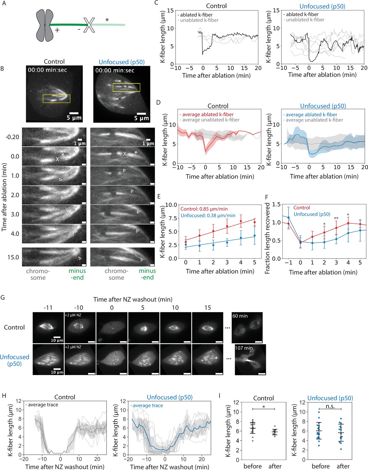
Kinetochore-fibers recover their lengths without focused poles.
See also Figure 2—videos 1 and 2. (A) Schematic of a k-fiber after ablation at position X. The k-fiber stub still attached to the chromosome persists with a new minus-end (dark green). The k-fiber segment closer to the pole with a new plus-end depolymerizes away (light green, *). (B) Representative confocal timelapse images of PtK2 k-fibers with GFP-α-tubulin and mCherry-p50 (in unfocused only). K-fibers were laser ablated at t = 0 (X) and followed over time. Empty arrowheads mark newly created minus-ends. (C) K-fiber lengths over time in a representative control and unfocused spindle. Gray traces represent unablated k-fibers. The ablated k-fiber is plotted in black. (D) Binned and averaged k-fiber lengths over time for ablated control and unfocused spindles. The average length of non-ablated k-fibers is plotted in gray, the average of ablated k-fibers in red for control and blue for unfocused. Shaded colors indicate ±1 standard deviation for their respective condition (Control: N = 7 cells, n = 8 ablated k-fibers, m = 26 non-ablated k-fibers; Unfocused: N = 6 cells, n = 8 ablated k-fibers, m = 31 non-ablated k-fibers). (E) Average growth rates of k-fibers immediately following ablation. Linear regression was performed on binned k-fiber lengths during the first 5 min following ablation (Control: 0.85 ± 0.09 µm/min, Unfocused: 0.38 ± 0.42 µm/min, p = 0.023). (F) Fraction of length recovered following ablation relative to the mean of unablated k-fibers in control and unfocused k-fibers. The average trace for unablated k-fibers in D was averaged over time and ablated lengths were normalized to this value. Times with statistically significant differences in length recovery are denoted by *. (G) Representative confocal timelapse images of PtK2 spindles with GFP-α-tubulin (in control and unfocused) and mCherry-p50 (in unfocused only), with 2 µM nocodazole added at −10 min and washed out at t = 0. (H) Lengths of k-fibers over time during nocodazole washout. All k-fibers are shown with the average trace plotted with ±1 standard deviation shaded in light gray (Control: N = 3 cells, n = 28 k-fibers; Unfocused: N = 4 cells, n = 23 k-fibers). (I) Mean k-fiber lengths before nocodazole and after washout in control and unfocused spindles (Control before: 6.58 ± 1.15 µm, n = 17; Control after: 5.76 ± 0.57 µm, n = 12, p = 0.02; Unfocused before: 6.03 ± 1.73 µm, n = 17; Unfocused after: 5.63 ± 1.80 µm, n = 14, p = 0.55). Numbers are mean ± standard deviation. Significance values determined by Welch’s two-tailed t-test denoted by * for p < 0.05, ** for p < 0.005, and *** for p < 0.0005.
-
Figure 2—source data 1
This spreadsheet contains the data used to generate plots 2C, 2D, 2E, 2F, and 2S1.
- https://cdn.elifesciences.org/articles/85208/elife-85208-fig2-data1-v3.xlsx
-
Figure 2—source data 2
This spreadsheet contains the data used to generate plots 2H and 2I.
- https://cdn.elifesciences.org/articles/85208/elife-85208-fig2-data2-v3.xlsx
Figure 2—figure supplement 1

Kinetochore-fiber lengths before ablation.
Lengths of k-fibers in unfocused cells prior to ablation. Lengths were measured in 3D from z-stacks of PtK2 cells expressing GFP-α-tubulin and mCherry-p50 taken by confocal live-imaging, as in Figure 1E. The dotted line represents the mean control k-fiber length as calculated in Figure 1E (N = 4 cells, n = 79 k-fibers, 7.60 ± 2.07 µm).
Figure 2—video 1
Ablating kinetochore-fibers: control vs. unfocused spindle.
Control (left) and unfocused (right) k-fibers grow back after being severed by a laser. See also Figure 2B. Live confocal imaging of a PtK2 cell expressing GFP-α-tubulin and mCherry-p50 (unfocused only). The ablation site is marked by ‘X’, causing the segment containing the old minus-end of the k-fiber to quickly depolymerize (‘*’). The new stable minus-end is tracked by the empty arrowhead. Time is in min:s, with ablation occurring at t = 0. Scale bar, 5 µm.
Figure 2—video 2
Spindle assembly after nocodazole washout: control vs. unfocused spindle.
Control (left) and unfocused (right) spindles grow back robustly after washing out nocodazole, a microtubule-destabilizing drug. See also Figure 2G. Live confocal imaging of a PtK2 cell expressing GFP-α-tubulin and mCherry-p50 (unfocused only). 2 µM nocodazole was added for 10 min before 10 washes in warmed media were started at t = 0. Time is in hr:min. Scale bar, 5 µm.
Figure 3 with 1 supplement
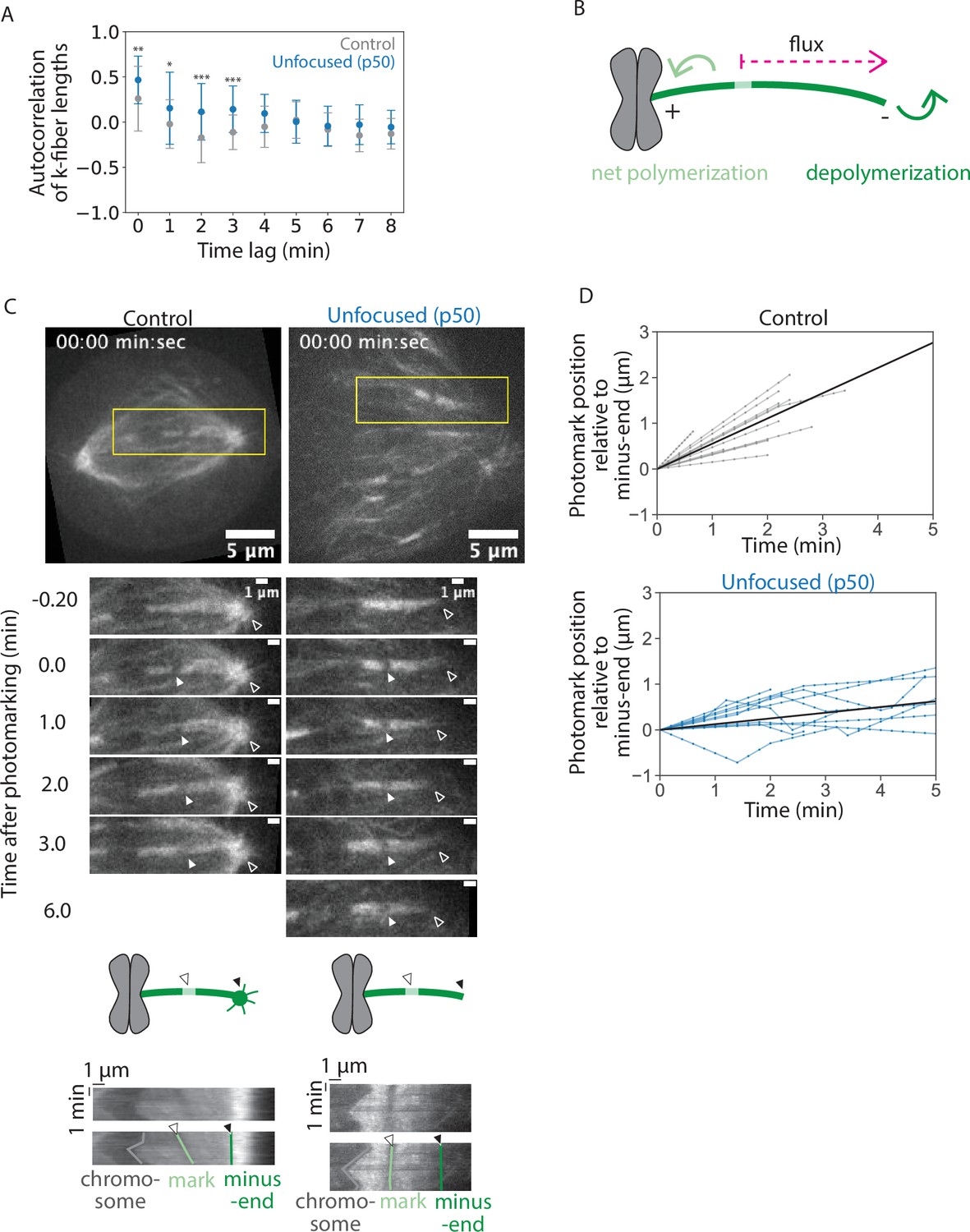
Kinetochore-fibers exhibit reduced end dynamics in the absence of poles and pole-focusing forces.
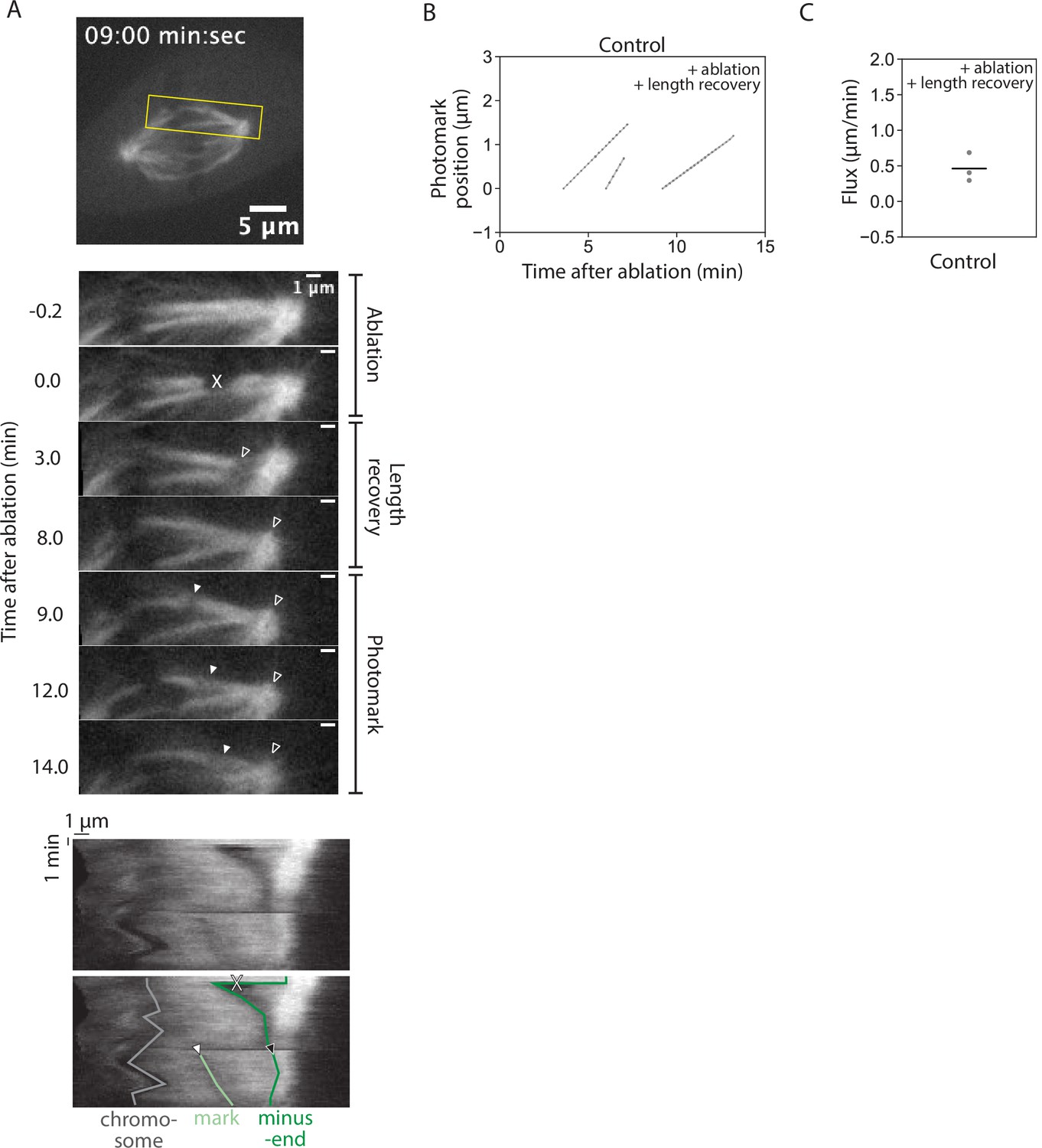
See also Figure 3—video 1. (A) Autocorrelation of k-fiber lengths over time from Figure 1H for control and unfocused k-fibers. Calculations and statistical analysis were performed using built-in Mathematica functions, where * indicates p < 0.05. (B) Schematic of a photomark (light green) on a k-fiber (dark green). The dotted arrow shows the direction the photomark moves with flux in control, where displacement of the mark toward the minus-end increases over time. Net end dynamics are shown by curved arrows (equal at steady state). (C) Representative confocal timelapse images of PtK2 k-fibers with GFP-α-tubulin (in control and unfocused) and mCherry-p50 (in unfocused only). A bleach mark was made at time = 0 and followed over time (filled arrowhead). Empty arrowheads indicate minus-ends. Below: Kymographs of the above images. Each row of pixels represents a max-intensity projection of a 5-pixel high stationary box drawn around the k-fiber at one time point (yellow box). (D) Minus-end dynamics, where photomark position over time describes how the mark approaches the k-fiber’s minus-end over time in control and unfocused k-fibers. Each trace represents one mark on one k-fiber. To measure flux as defined by minus-end depolymerization, the movement of the photomark toward the minus-end was plotted over time. Line with the average slope is drawn in black (Control: N = 8 cells, n = 12 k-fibers; Unfocused: N = 8 cells, n = 11 k-fibers). Numbers are mean ± standard deviation. Significance values determined by Welch’s two-tailed t-test denoted by n.s. for p ≥ 0.05, * for p < 0.05, ** for p < 0.005, and *** for p < 0.0005.
-
Figure 3—source data 1
This spreadsheet contains the data used to generate plot 3D.
- https://cdn.elifesciences.org/articles/85208/elife-85208-fig3-data1-v3.xlsx
Figure 3—video 1
Photobleaching kinetochore-fibers to measure microtubule flux: control vs. unfocused spindle.
Control (left) and unfocused (right) k-fibers exhibit poleward flux (reduced in unfocused spindles) as demonstrated by a bleach mark on a k-fiber moving toward a pole over time. See also Figure 3C. Live confocal imaging of a PtK2 cell expressing GFP-α-tubulin and mCherry-p50 (unfocused only). The laser-induced bleach mark is tracked by the filled arrowhead over time as its associated tubulin moves away from the kinetochore toward the minus-end (empty arrowhead). Time is in min:s, with the photomark created at t = 0. Scale bar, 5 µm.
Figure 4 with 3 supplements
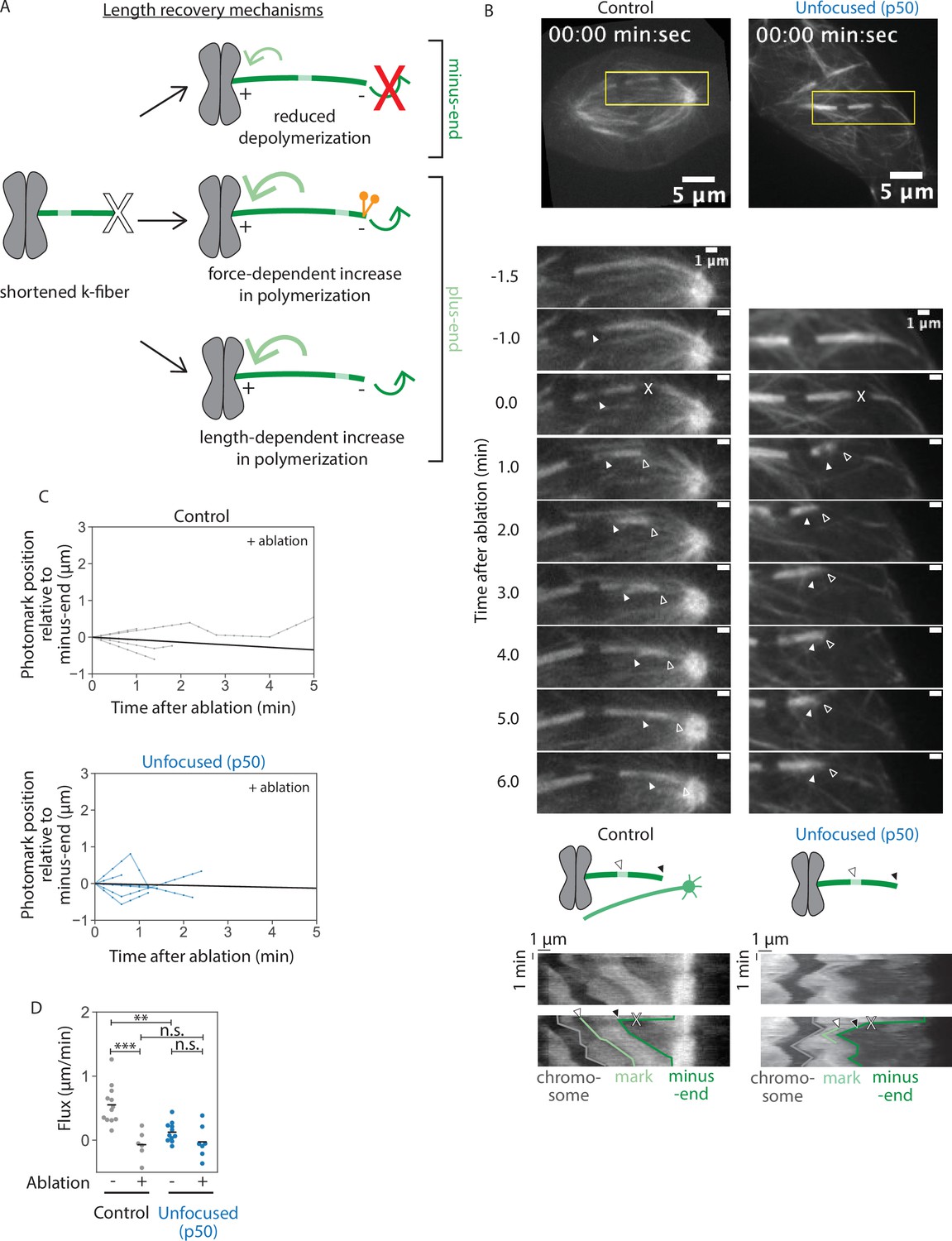
Kinetochore-fibers tune their end dynamics to recover length, without pole-focusing forces.
See also Figure 4—video 1. (A) Models describing k-fiber length recovery mechanisms. K-fibers shortened by ablation (X) with a photomark (light green) can potentially grow back in different ways: suppression of minus-end depolymerization (top), increased plus-end polymerization induced by forces such as dynein (middle), or increased polymerization in a length-dependent manner (bottom). (B) Representative confocal timelapse images of PtK2 k-fibers with GFP-α-tubulin (in control and unfocused) and mCherry-p50 (in unfocused only). Filled arrowhead follows a bleach mark. At t = 0, k-fibers were cut with a pulsed laser at higher power (X). Empty arrowhead follows the new k-fiber minus-end. Below: Kymographs of the above images as prepared in Figure 3C. (C) Minus-end dynamics were probed by tracking movement of the mark toward the k-fiber’s minus-end over time in control and unfocused k-fibers after ablation at t = 0. Line with the average slope is drawn in black (Control: N = 5 cells, n = 6 k-fibers; Unfocused: N = 7 cells, n = 7 k-fibers). (D) Minus-end dynamics of k-fibers. Flux as measured by rate of photomark movement toward the minus-end with or without ablation in control and unfocused k-fibers. Each point represents the slope of one trace in Figure 3D or (C) measured by linear regression (Control: mean flux = 0.55 ± 0.29 µm/min, mean flux after ablation = −0.07 ± 0.20 µm/min; Unfocused: mean flux = 0.13 ± 0.15 µm/min, mean flux after ablation = −0.03 ± 0.23 µm/min; p non-ablated control vs. ablated control = 2.7e−4, p non-ablated control vs. non-ablated unfocused = 5.3e−4, p non-ablated unfocused vs. ablated unfocused = 0.19, p ablated control vs. ablated unfocused = 0.75). Numbers are mean ± standard deviation. Significance values determined by Welch’s two-tailed t-test denoted by n.s. for p ≥ 0.05, * for p < 0.05, ** for p < 0.005, and *** for p < 0.0005.
-
Figure 4—source data 1
This spreadsheet contains the data used to generate plots 4C and 4D.
- https://cdn.elifesciences.org/articles/85208/elife-85208-fig4-data1-v3.xlsx
Figure 4—figure supplement 1
Minus-end depolymerization resumes after length recovery following ablation.
See also Figure 4—video 2. (A) Representative confocal timelapse images of PtK2 k-fibers with GFP-α-tubulin. At t = 0, k-fibers were cut with a pulsed laser at a high power (X). Empty arrowhead follows the new k-fiber minus-end. Filled arrowhead follows a bleach mark made several minutes later with the laser at a lower power. Below: Kymographs of the above images as prepared in Figure 3C. (B) Minus-end dynamics were probed by tracking movement of the mark relative to the k-fiber’s minus-end over time in control k-fibers several minutes after ablation (t = 0) once k-fiber repair and length recovery were complete. (C) Minus-end dynamics of k-fibers. Flux as measured by rate of photomark movement toward the minus-end after ablation and length recovery in control k-fibers. Each point represents the slope of one trace in (B) measured by linear regression (n = 3 cells, mean = 0.46 ± 0.16 µm/min).
-
Figure 4—figure supplement 1—source data 1
This spreadsheet contains the data used to generate plot 4S1.
- https://cdn.elifesciences.org/articles/85208/elife-85208-fig4-figsupp1-data1-v3.xlsx
Figure 4—video 1
Ablating and photomarking kinetochore-fibers: control vs. unfocused spindle.
Control (left) and unfocused (right) k-fibers exhibit no measurable minus-end depolymerization during regrowth after ablation. See also Figure 4B. Live confocal imaging of a PtK2 cell expressing GFP-α-tubulin and mCherry-p50 (unfocused only). The ablation site is marked by ‘X’ and the new stable minus-end is tracked by the empty arrowhead. The photomark is tracked by the filled arrowhead and it does not appear to get closer to the other arrowhead at the minus-end over time. Time is in min:s, with ablation occurring at t = 0. Scale bar, 5 µm.
Figure 4—video 2
Photobleaching control kinetochore-fibers after ablation and length recovery.
Control k-fibers resume minus-end depolymerization after ablation and length recovery. See also Figure 4—figure supplement 1. Live confocal imaging of a PtK2 cell expressing GFP-α-tubulin. The ablation site is marked by ‘X’ and the new stable minus-end is tracked by the empty arrowhead. The photomark is made several minutes after ablation when k-fiber repair and length recovery are complete. The mark is tracked by the filled arrowhead as it approaches the other arrowhead at the minus-end over time. Time is in min:s, with ablation occurring at t = 0. Scale bar, 5 µm.
Figure 5 with 1 supplement
Spindle poles coordinate chromosome segregation and cytokinesis.
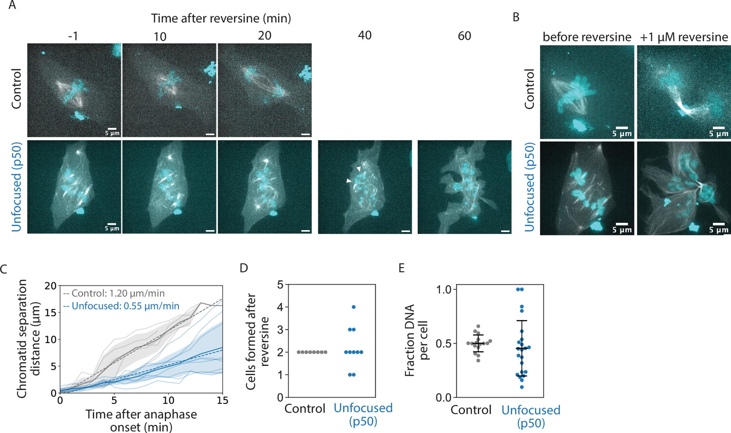
See also Figure 4—video 1. (A) Representative confocal timelapse images of PtK2 spindles with GFP-α-tubulin (in control and unfocused) and mCherry-p50 (in unfocused only) treated with 0.1 or 0.5 µM SiR-DNA with 1 µM reversine added at t = 0. Arrowheads depict an example of sister chromatids separating, later measured in C. (B) Max-intensity z-projections before adding reversine and 20 min after anaphase onset for the control and unfocused spindle in A. Figures C–E are from the same dataset (Control: N = 8 dividing cells; Unfocused: N = 10 dividing cells). (C) Sister chromatid separation velocity. For the chromatid pairs that were observed to separate, sister chromatid distance over time was measured for focused and unfocused spindles starting at anaphase onset. Control is plotted in gray, unfocused in blue. Light-colored traces represent one separating chromatid pair, with their average plotted as a dark line with shading representing ±1 standard deviation. The line of best fit for each condition averaged is shown as a dotted line, with their slopes shown (Control: N = 4 dividing cells, n = 5 chromosome pairs, separation velocity = 1.20 µm/min; Unfocused: N = 3 dividing cells, n = 9 chromatid pairs, separation velocity = 0.55 µm/min). (D) Number of ‘cells’ formed after cytokinesis in reversine-treated control and unfocused spindles (Control: 2 ± 0 cells; Unfocused: 2.20 ± 0.87 ‘cells’). (E) Fraction of chromosome mass per ‘cell’ after reversine treatment. Summed z-projections of chromosome masses were used to calculate the fraction of chromosome mass per cell (Control: 0.50 ± 0.08 a.u.; Unfocused: 0.45 ± 0.26 a.u.). Numbers are mean ± standard deviation.
-
Figure 5—source data 1
This spreadsheet contains the data used to generate plots 5C, 5D, and 5E.
- https://cdn.elifesciences.org/articles/85208/elife-85208-fig5-data1-v3.xlsx
Figure 5—video 1
A reversine-treated control spindle undergoing anaphase: control vs. unfocused spindle.
Control (left) and unfocused (right) spindles treated with a cell cycle checkpoint inhibitor enter anaphase and segregate chromosomes. See also Figure 5A. Live confocal imaging of a PtK2 cell labeled with SiR-DNA (cyan) and expressing GFP-α-tubulin and mCherry-p50 (unfocused only) with 1 µM reversine added. Time is in min:s, with reversine added at t = 0. Scale bar, 5 µm.
Figure 6
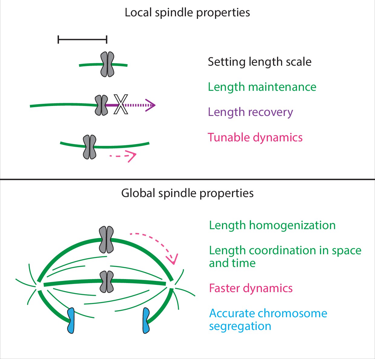
Spindle length is a local spindle property and length coordination is a global spindle property.
Cartoon summary of spindle properties set locally vs. globally. Setting, maintaining, and recovering length is regulated by individual k-fibers locally, independently of poles and pole-focusing forces. In turn, coordinating lengths across space and time requires global cues from focused poles. In sum, spindle length emerges locally, but spindle coordination emerges globally.
Tables
Key resources table
| Reagent type (species) or resource | Designation | Source or reference | Identifiers | Additional information |
|---|---|---|---|---|
| Cell line (P. tridactylus, male) | PtK2 | Gift from T. Mitchison, Harvard University | PMID:1633624 | Kidney epithelial |
| Cell line (P. tridactylus, male) | HaloTag-tubulin PtK2 | This paper | Kidney epithelial | |
| Cell line (H. sapiens, female) | RPE1 | ATCC | ATCC Cat#CRL-4000; RRID: CVCL_4388 | Retina, epithelial |
| Chemical compound, drug | Nocodazole | Sigma | M1404 | Final concentration 2 µM |
| Chemical compound, drug | Reversine | Sigma | R3904 | Final concentration 1 µM |
| Chemical compound, drug | Viafect | ProMega | E4981 | 1:6 ratio of Viafect:DNA used |
| Chemical compound, drug | Janelia Fluor 646 | Janelia | 6148 | Final concentration 100 nM |
| Chemical compound, drug | SiR-DNA | Spirochrome | SC007 | Final concentration 0.1–0.5 µM with 1 µM verapamil |
| Chemical compound, drug | SiR-tubulin | Spirochrome | SC002 | Final concentration 0.1 µM with 1 µM verapamil |
| Recombinant DNA reagent | pLV-β-tubulin-HaloTag (plasmid) | This paper | Lentiviral plasmid. Progenitors: Addgene #114021 (Geert Kops) and Addgene #64691 (Yasushi Okada) | |
| Recombinant DNA reagent | pLV-mCherry-p50 (plasmid) | This paper | Lentiviral plasmid. Progenitors: Addgene #114021 (Geert Kops) and mCherry-p50 (PMID:19196984) | |
| Recombinant DNA reagent | eGFP-α-tubulin (plasmid) | Michael Davidson collection given to UCSF; Rizzo et al., 2009 | Addgene Plasmid #56450 | |
| Recombinant DNA reagent | mCherry-p50 (plasmid) | Gift from M. Meffert, Johns Hopkins University; | PMID:19196984 | |
| Recombinant DNA reagent | β-Tubulin HaloTag (plasmid) | Addgene; Uno et al., 2014 | Addgene Plasmid #64691 | |
| Software, algorithm | FIJI | FIJI; Schindelin et al., 2012 | ImageJ version 2.1.0 | |
| Software, algorithm | Wolfram Mathematica | Wolfram Mathematica | Version 13.0 | |
| Software, algorithm | MetaMorph | MDS Analytical Technologies | Version 7.8 | |
| Software, algorithm | Micro-Manager | Micro-Manager; Edelstein et al., 2010 | Version 2.0.0 | |
| Software, algorithm | Python | Python | Version 3.8.1 | Spyder IDE version 4.1.5 |
Additional files
Download links
A two-part list of links to download the article, or parts of the article, in various formats.
Downloads (link to download the article as PDF)
Open citations (links to open the citations from this article in various online reference manager services)
Cite this article (links to download the citations from this article in formats compatible with various reference manager tools)
Kinetochore-fiber lengths are maintained locally but coordinated globally by poles in the mammalian spindle
eLife 12:e85208.
https://doi.org/10.7554/eLife.85208


