Unified quantitative characterization of epithelial tissue development
- Institut Curie, France
- Meiji University, Japan
- Kyoto University, Japan
- Japan Science and Technology Agency, Japan
- Université Paris-Diderot, France
Figures
Figure 1 with 1 supplement
Definitions of the main formalism quantities and analysis workflow.
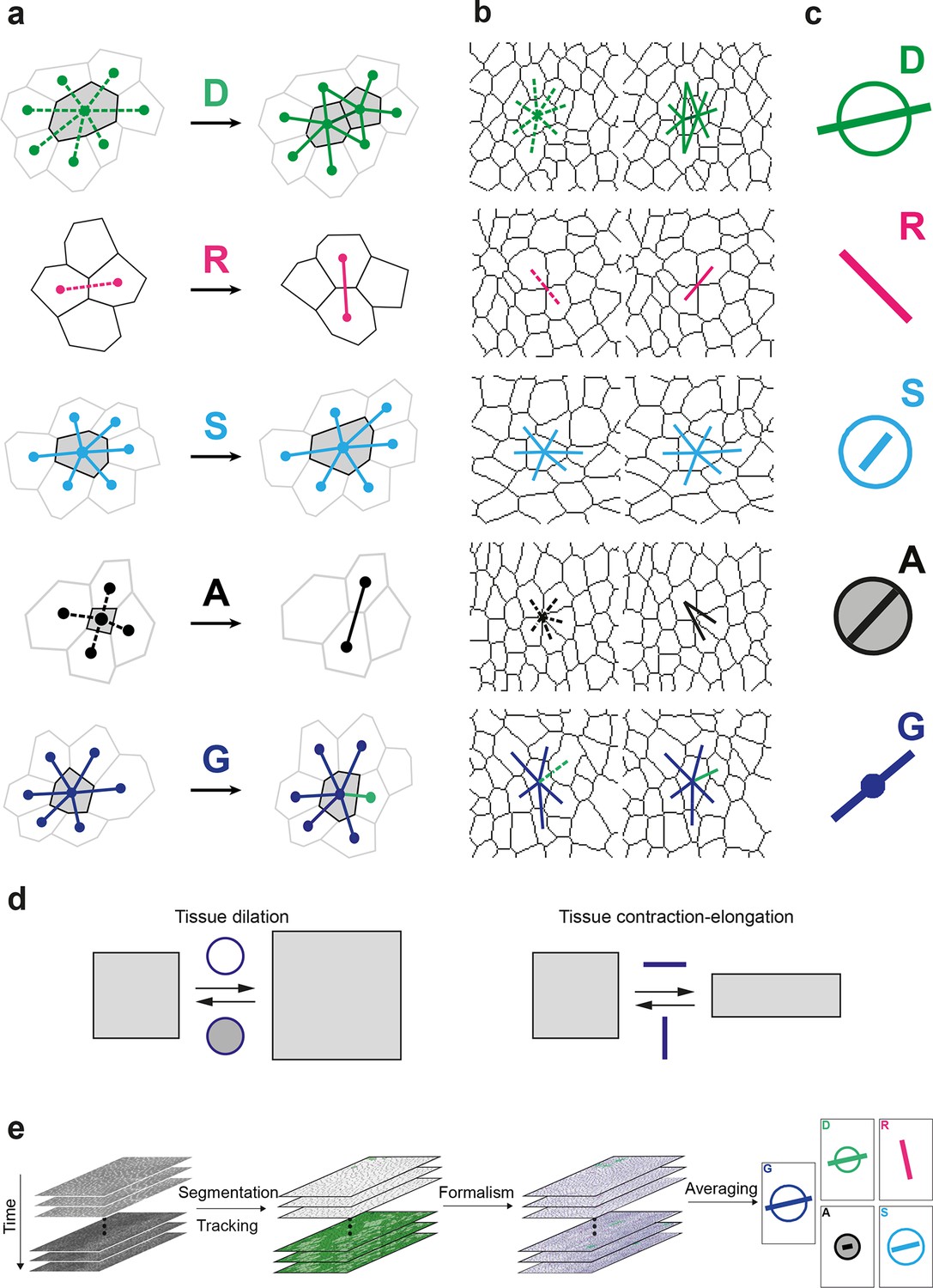
(a) Characterizations of the four main elementary cell processes and of tissue deformation: divisions (green; and dark green for the link created between the daughter cells); , rearrangements (magenta); , size and shape changes (cyan); , apoptosis/delaminations (black). They are defined and measured from the rates of changes in length, direction and number of cell-cell links, here on two schematized successive images. They make up the tissue deformation rate , the measurement of which is based on geometric changes of conserved links (dark blue links) excluding non-conserved links (green). Dots indicate cell centroids. Lines are links between neighbor cell centroids. Dashes are links on the first image (left) which are no longer present on the second one (right). Some cells are hatched in grey to facilitate the comparison. (b) Measurements of the four elementary main cell processes rates and of tissue deformation rate. Same as (a), this time showing cell-cell links on two actual successive segmented images extracted from experimental time-lapse movies. (c) Representation with circles and bars of the quantitative measurements performed on (b) of the deformation rates explained in (d). (d) Deformation rate: a deformation quantifies a relative change in tissue dimensions: it is expressed without unit, e.g. as percents. A deformation rate is thus expressed as the inverse of a time, e.g. 10-2 h-1 represents a 1% change in dimension within one hour. It can be decomposed into two parts. First (left): an isotropic part that relates to local changes in size. The isotropic part can either be positive or negative, reflecting a local isotropic growth or shrinkage of the tissue. The rate of dilation is represented by a circle, the diameter of which scales with the magnitude of the rate. Positive and negative dilations are represented by circles filled with white and grey, respectively. Second (right): an anisotropic part that relates to local changes in shape. The anisotropic part of the deformation rate quantifies the local contraction-elongation or convergence-extension (CE) without change in size. It can be represented by a bar in the direction of the elongation, the length and direction of which quantify the magnitude and the orientation of the elongation. (e) Workflow used to quantify tissue development. Image analysis leads to characterization of cell contours (segmentation), and lineages (tracking) in the case of movies. Our formalism yields an identification of each cell-level process and its description in terms of cell-cell links (see a–b) and a quantitative measurement of their associated deformation rate (see c–d). Averaging over time, space and/or movies of different animals yields a map of each quantity in each region of space at each time with a good signal-to-noise ratio (see Videos 1, 4, 5).
Figure 1—figure supplement 1
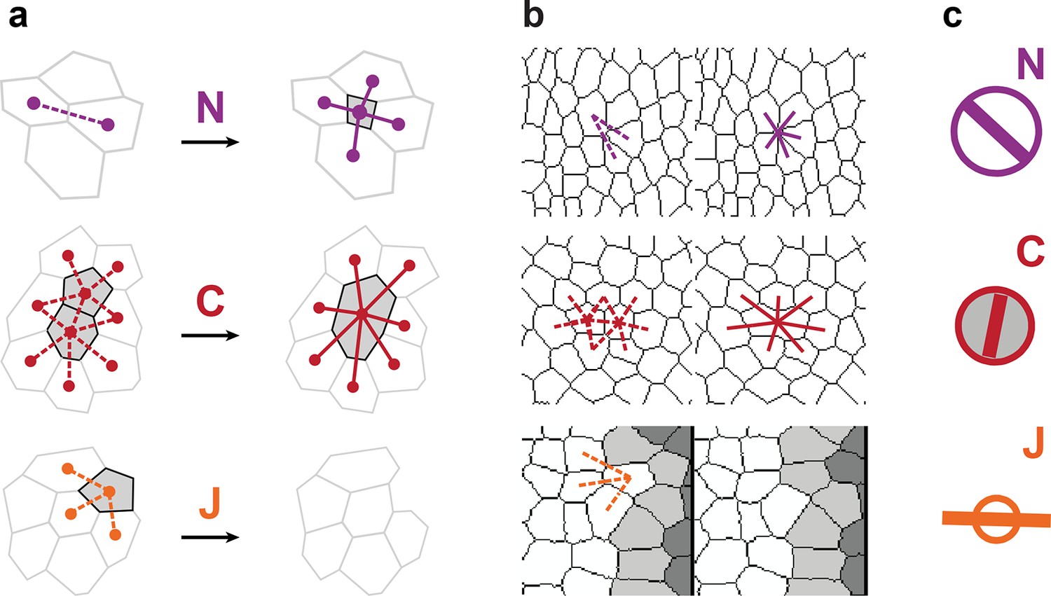
Characterizations of the additional elementary cell processes , , .
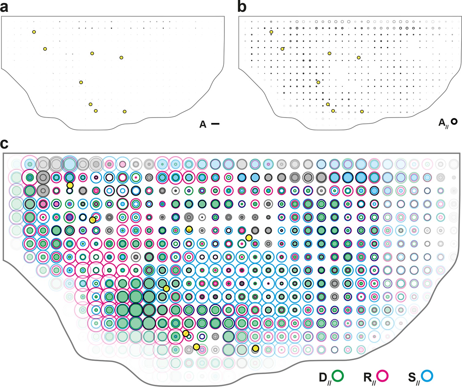
(a) The new cell integration (purple), cell fusion (crimson), cell flux through tissue boundaries (grey) on two schematized successive images. Dots indicate cell centroids. Lines are links between neighbor cell centroids. Dashes are links on the first image (left) which are no longer present on the second one (right). Some cells are hatched in grey to facilitate the comparison. (b) Measurements of the three additional cell processes rates. Same as (a), this time showing cell-cell links on two actual successive segmented images extracted from experimental time-lapse movies. is defined through links which cross the boundary of the field of view. Dark grey cells are boundary cells, partly out of the field of view, and their centroids are not defined. Light grey cells touch a boundary cell : their links with dark grey cells are ill-defined and are therefore excluded from calculations. (c) Representation with circles and bars of the quantitative measurements performed on (b) of the deformation rates explained in Figure 1d.
Figure 2 with 1 supplement
Computer simulations validating the quantitative characterizations of the main cell processes and tissue deformation.
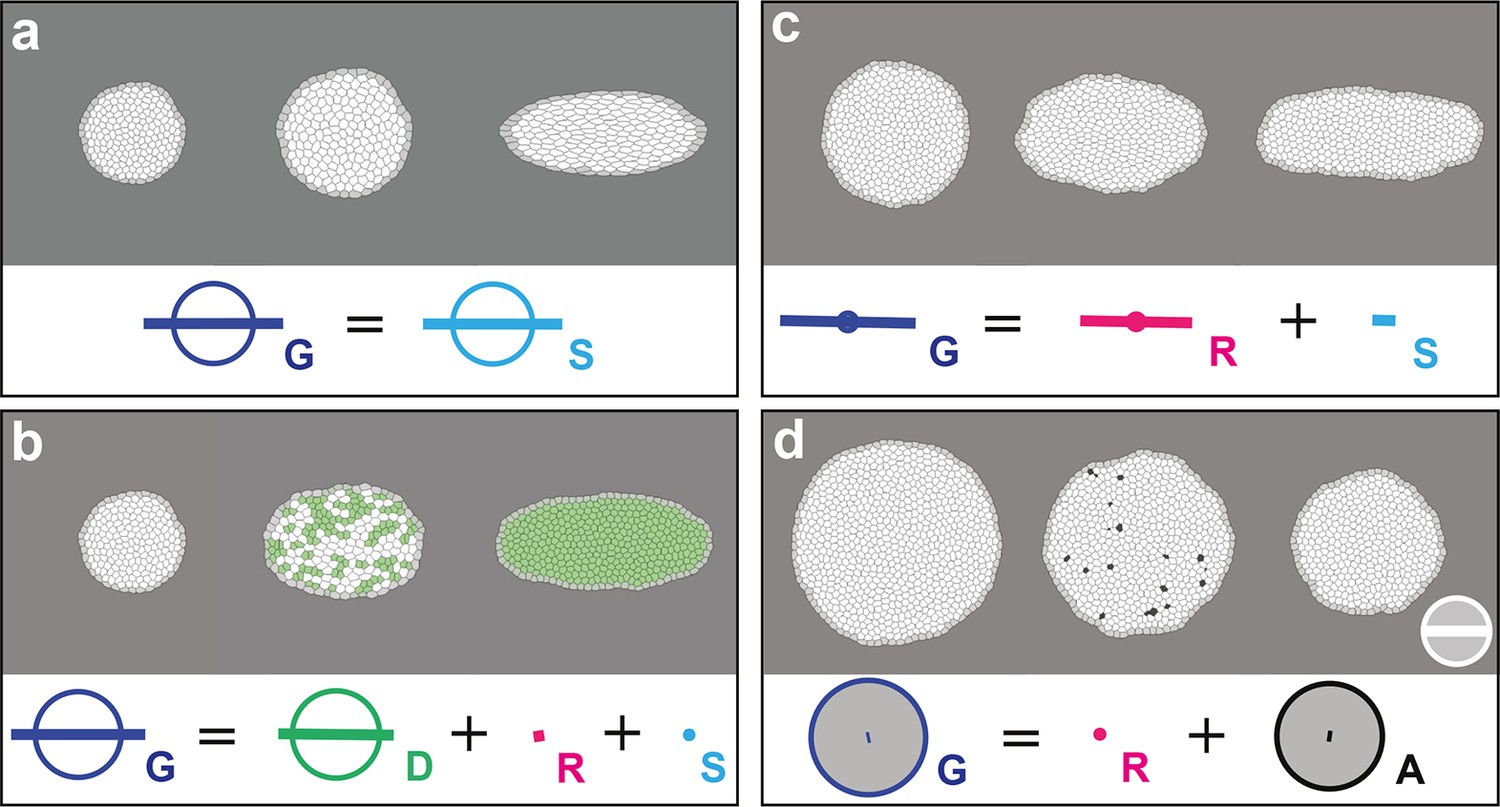
In (a–d), upper panels: simulated deformation of a cell patch; left: initial state of the simulation; middle: intermediate state; right: final state. Lower panels: Equation 1 is visually displayed. (a) By direct image manipulation (hence not followed by any cell shape relaxation), the initial pattern (left) is dilated (middle) then stretched (right) with known dilation and CE rates, thereby solely generating the same size and shape changes for the patch and for each individual cell. The patch deformation rate and the cell size and shape change rate are measured independantly with 0.3% of error, and, as expected when no topological changes occur, we find . This validates the measurement of and , which in turn validates the other measurements in the next simulations. (b) Potts model simulation of oriented cell divisions. Forces are numerically implemented along the horizontal axis. They drive the elongation of the cell patch while each cell divides once along the same axis. Therefore both and have their anisotropic parts along the horizontal direction. The residual cell rearrangements and cell shape changes CE rates and are respectively due to some cell rearrangements actually occurring in the simulation, and to some cells having not completely relaxed to their initial sizes and shapes. This is not due to any entanglement between the cell process measurements in the formalism. Divided cells are in green. (c) Potts model simulation of oriented cell rearrangements. The same forces as in (b) drive the elongation of the cell patch first leading to the elongation of cells that then relax their shape by undergoing oriented rearrangements along the same axis, thereby leading to both and having their anisotropic parts along the horizontal direction. The cell shape relaxation is not complete as cells remain slightly elongated by the end of the simulation (right), thereby giving a residual . (d) Potts model simulation of cell delaminations. Delaminations were obtained by gradually decreasing the cell target areas of half the cells of the initial patch to 0, thereby driving the isotropic shrinkage of the patch to half of its initial size. It leads to equal negative growth rates for and , up to residual other processes. Delaminating cells are in black. The white scale bar and circle in (d) both correspond respectively to CE and growth rates of 10-2 h-1 for simulation movies lasting 20 h, in all panels (a–d). Only measurements with norm > 10-3 h-1 have been plotted.
Figure 2—figure supplement 1
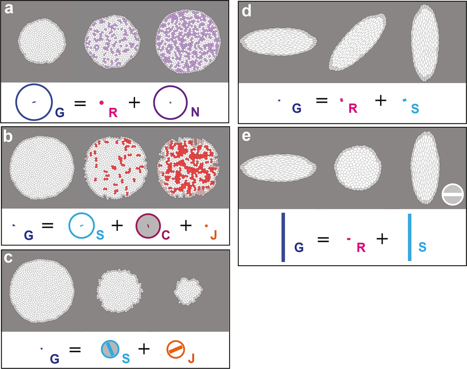
Computer simulations validating the quantitative characterization of the additional cell processes , , and testing rotation.
In (a–c), upper panels, simulated deformation of a cell patch. Left: initial state of the simulation; middle: intermediate state; right: final state. Lower panels: Equation 15 is visually displayed. (a) Simulation of patch growth via new cell integration , produced by time-reversal of the delamination simulation (Figure 2d), thereby leading to equal positive growth rates for and , up to residual other processes. (b) Simulation of patch undergoing cell fusion , produced by the random removal of cell-cell junctions. In this particular example, the patch undergoes no deformation at all, while the removal of junctions lead to an artificial increase of average cell size measured by a positive cell growth rate , and an opposite fusion rate that cancels it, thus leading to . This validates measurement since has been validated in Figure 2a. (c) Simulation of cell outward flux . Outer layers of cells of the patch are progressively removed, and there is again virtually no morphogenesis like in (b). The small cell size and shape changes measured is due to the smaller number of cells over which it is averaged and is completely compensated by the flux term , leading to . (d) By direct image manipulation using an image treatment software, an initially elongated pattern (left, identical to the final pattern of Figure 2a) is rotated anticlockwise by 90° (right). This validates that for rigid body movements such as a rotation, the formalism does not detect any significant CE rates, as expected. (e) For comparison with (d), by direct image manipulation using an image treatment software, the same initial elongated pattern of (d) is now brought to a round pattern (middle) by a convergence-extension, and is then stretched again by the same convergence-extension, which leads to its elongation in the perpendicular direction, resulting in a final pattern very similar to the one in (d), with same aspect ratio (right). This illustrates that for such a pure CE without rotation, the formalism does detect significant CE rates for and as expected, although the initial and final states are very similar to (d). This also illustrates that all our measurements depend on the deformation path between the initial and final states. The white scale bar in (e) is equivalent to: (a,d) 10-2 h-1, (c) 0.1 10-2 h-1, (b,e) 2 10-2 h-1. Only measurements with norm > 10-3 h-1 have been plotted.
Figure 3 with 2 supplements

Quantitative characterization of tissue morphogenesis of the whole Drosophila notum.
(a) Drosophila adult fly. Yellow dotted box is the notum, circles filled in yellow are macrochaetae. (b) Drosophila pupa. Yellow dotted box is the region that was filmed. Black dotted line is the midline (along the anterio-posterior direction, mirror symmetry line for the medial-lateral axis). (c) Rate of cell divisions obtained from cell tracking. Number of cell divisions color-coded on the last image of the movie (28 hAPF), light green cell: one division; medium green cell: two divisions; dark green cells: three divisions and more; purple cells: cells entering the field of view during the movie. Circles filled in yellow indicate macrochaetae. The other white cells are microchaetae. (d) Growth and morphogenesis of cell patches during notum development. (Left) Cell contours (thin grey outlines) at 14 hAPF. A grid made of square regions of 40 μm sides was overlayed on the notum to define patches of cells whose centers initially lied withing each region (∼30 cells per patch in the initial image). Within each patch, all cells (and their future offspring) were assigned a given color. The assignement of patch colors was arbitrary but nevertheless respected the symmetry with respect to the midline (in cyan) to make easier the pairwise comparison of patches. Each patch was then tracked as it deformed over time to visualize tissue deformations at the patch scale. (Right) Cell contours at 28 hAPF. The variety of patch shapes reveals the heterogeneity of deformations at the tissue scale, as well as their striking symmetry with respect to the midline. (e) Map of average cell division orientation (bar direction) and anisotropy (bar length), (Appendix C.3.2). Its determination is solely based on the links between newly appeared sister cells (link in dark green in Figure 1a,b). (f–j) Maps of orientation (bar direction) and anisotropy (bar length) of CE rates, for (f) the tissue (compare the bar amplitude and orientation pattern with the pattern of patches in (d) right), (g) cell divisions , (h) cell rearrangements , (i) cell shape changes and (j) delaminations . In this Figure (and Figure 3—figure supplements 1 and 2), measurements over the whole notum have been averaged over 14 h of development (between 14 and 28 hAPF) and plotted on the last image of the movie (for their time-evolution see Video 4); contours of cells (thin grey outlines) and of initially square patches (thick grey outlines); black boxes outline the posterior regions (medial and lateral) described in the text; patches near the tissue boundary contain less data and are plotted accordingly with higher transparency; circles filled in yellow indicate macrochaetae; dashed black line is the midline. Scale bars: (a,b) 250 μm, (c,d) 50 μm, (e–j) 2 10-2 h-1.
Figure 3—figure supplement 1
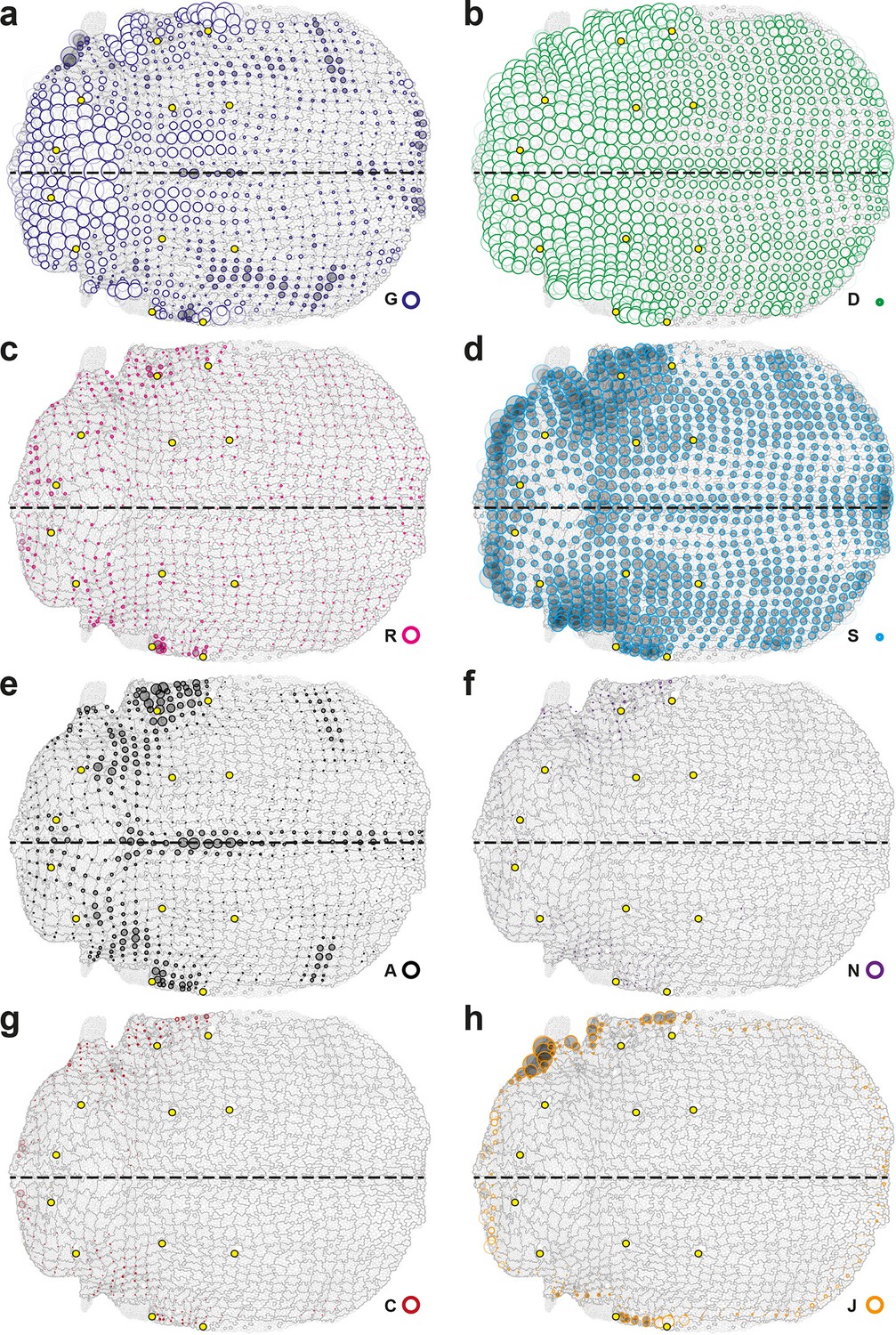
Complete set of maps of dilation rates (isotropic parts of measurements).
The additivity (Equation 15) also applies separately to these isotropic parts. Circle diameters are proportional to the traces of: (a) tissue dilation , (b) cell divisions , (c) cell rearrangements , (d) cell size changes , (e) delaminations , (f) new cell integrations , (g) fusions , (h) boundary flux . Scale circle diameters: 2 10-2 h-1. Note that the isotropic part of cell divisions is always positive and that of delaminations is always negative, as expected.
Figure 3—figure supplement 2
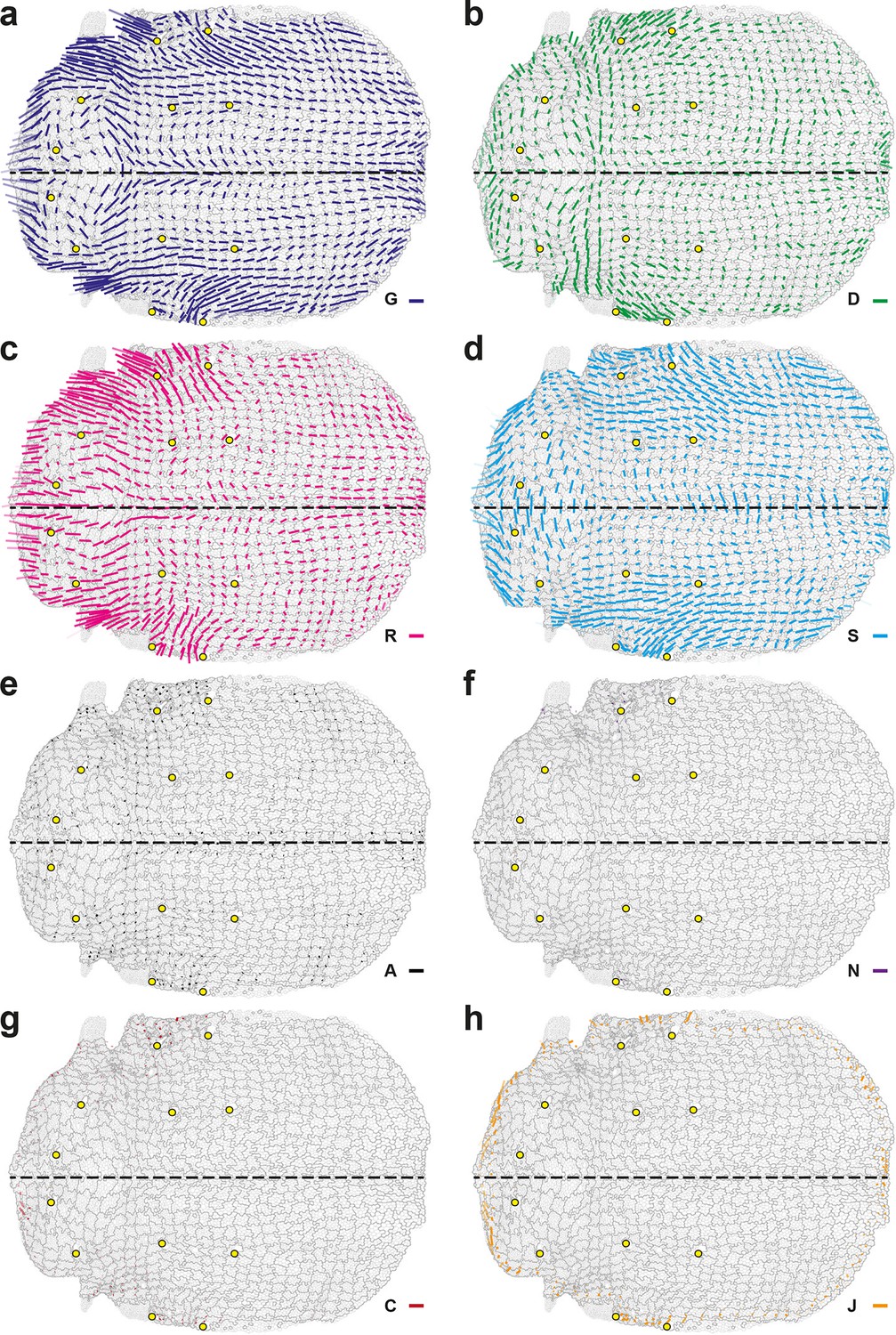
Complete set of maps of contraction-elongation (CE) rates (anisotropic parts of measurements).
The additivity (Equation 15) also applies separately to these anisotropic parts. Panels already presented in the Figure 3f–j are replotted here (a–e) for comparison with additional measurements (f–h): (f) new cell integrations , (g) fusions , (h) boundary flux . Scale bars: 2 10-2 h-1.
Figure 4 with 1 supplement

Quantifications of tissue and cell process deformations during tissue development, averaged over 5 hemi-nota.
(a,b) Average maps of CE rates of (a) the tissue (, dark blue) and of (b) cell divisions (, green), cell rearrangements (, magenta) and cell shape changes (, cyan) overlayed for comparison. Time averages were performed between 14 and 28 hAPF. Scale bars: 2 10-2 h-1. In this Figure (and Figure 4—figure supplement 1), values larger than the local biological variability are plotted in color while smaller ones are shown in grey; a local transparency is applied to weight the CE rate according to the number of cells and hemi-nota in each group of cells; black outline delineates the archetype hemi-notum; the midline is the top boundary; circles filled in yellow are archetype macrochaetae. Black rectangular boxes outline the four regions numbered 1 to 4 described in the text. (c) Projection of a cell process along the local axis of tissue elongation: cell process component. Here, is unitary and has the direction of the local tissue CE rate : its bar therefore indicates the local direction of tissue elongation (Equation 16). For each cell process measurement , its component along can be determined by its projection onto and is noted (Equation 17). It is expressed as a rate of change per unit time, i.e. in hour-1, and is represented as a circle whose area is proportional to the component. (Left) If a cell process CE rate (here orange bar) is rather parallel to (dark blue bar), it has a positive component on (orange empty circle). (Middle) If the bar is at 45° angle to , its component on is zero. (Right) If the CE rate bar is rather perpendicular to , its CE rate has a negative component on (orange full circle). Note that the component of tissue CE rate along itself, , is the amplitude of tissue CE rate , and is positive by construction. The additivity of cell process CE rates to (Equation 1) implies the additivity of these components to (Equation 2). Note also that these circles have a different meaning from those used to represent the dilation rates (Figure 1d). (d–g) Maps of components along the tissue CE rate for (d) the tissue rate itself (, dark blue, components are positive by construction) and of (e) cell divisions (, green), (f) cell rearrangements (, magenta) and (g) cell shape changes (, cyan). Same representation as in (a,b). Scale bars: 0.1 h-1. (h–k) Time evolution of components along the tissue CE rate of the tissue rate itself (, dark blue) and of cell divisions (, green), cell rearrangements (, magenta), cell shape changes (, cyan) and delaminations (, black) in four regions of interest. Measurements are averaged over sliding time windows of 2 h and spatially over the region (h) 1, (i) 2, (j) 3, (k) 4. In region 1, one can distinguish three phases where tissue morphogenesis mostly occurs via: (14–18 hAPF) cell rearrangements as divisions and cell shape changes nearly cancel out; (18–23 hAPF) cell shape changes, and it reaches its peak; (23–26 hAPF) oriented cell divisions as cell rearrangements and cell shape changes cancel out. In region 2, the same temporal phases can be distinguished: (14–18 hAPF) the effect of divisions is almost cancelled by cell shape changes; (18–22 hAPF) only weak changes occur; (22–26 hAPF) cell rearrangements and cell shape changes add up and morphogenesis becomes significant. In region 3, like in region 1, the two waves of oriented cell divisions can be seen clearly with peaks occurring around 16 and 23 hAPF, but here both division waves have a negative component along tissue CE rate. Cell rearrangements and cell shape changes make up for the negative sign of divisions, thereby mostly accounting for tissue morphogenesis in this region. In region 4, from about 18 hAPF onwards, the tissue CE rate significantly increases and almost perfectly overlaps with cell shape change CE rate, meaning that tissue morphogenesis solely occurs via cell shape changes.
Figure 4—figure supplement 1
Maps of delamination CE rate and overlay of maps of main cell process components along the tissue CE rate.
(a) Delaminations CE rate (, black), (b) corresponding component along the tissue CE rate, ; averages over 5 hemi-nota. Over this time period, delaminations therefore hardly participate in tissue morphogenesis. (c) Component along the tissue CE rate of cell divisions (, green), cell rearrangements (, magenta) and cell shape changes (, cyan) overlayed for comparison. Time averages were performed between 14 and 28 hAPF. Scale bar (a) 2 10-2 h-1; scale circle area (b,c) 0.1 h-1.
Figure 5 with 1 supplement
Quantitative characterization of pupal wing morphogenesis.
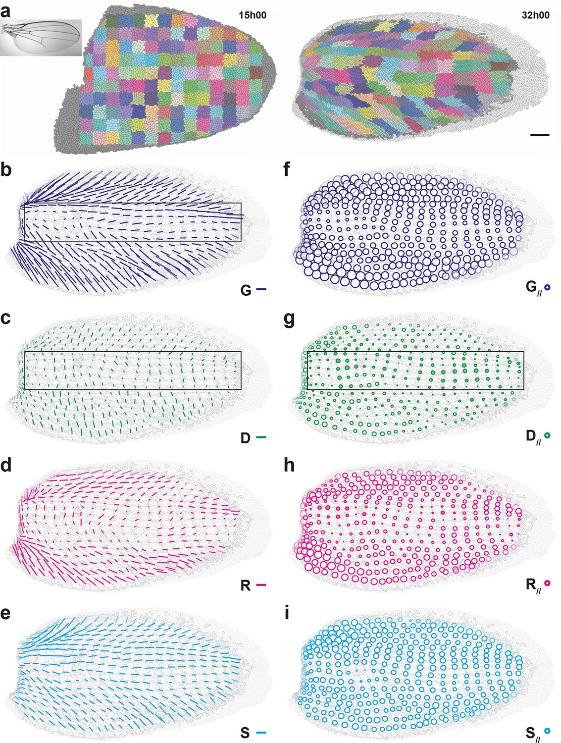
(a) Growth and morphogenesis of cell patches during wing development. (Left) Cell contours (thin grey outlines) at 15 hAPF. A grid made of square regions of 34 μm side was overlayed on the wing, to define patches of cells whose centers initially lied withing each region (∼30 cells per patch in the initial image). Within each patch, all cells (and their offspring) were assigned the same arbitrary color. Each patch was then tracked as it deformed over time to visualize tissue deformations at the patch scale. Inset: Drosophila adult wing. (Right) Cell contours at 32 hAPF. In this tissue as well, the variety of patch shapes reveals the heterogeneity of deformations at the tissue scale. (b–i) Average maps of main cell process CE rates (b–e) and of their components along tissue CE rate (f–i) for the CE rates of the tissue (, dark blue, b,f), cell divisions (, green, c,g), cell rearrangements (, magenta, d,h) and cell shape changes (, cyan, e,i). Black rectangular box in (b,c,g) outlines the region described in the text. Time averages were performed between 15 and 32 hAPF. A local transparency is applied to weight the CE rate according to the number of cells in each group of cells. Scale bars: (a) 50 μm, (b–e) 0.1 h-1; scale circle area (f–i) 0.1 h-1.
Figure 5—figure supplement 1
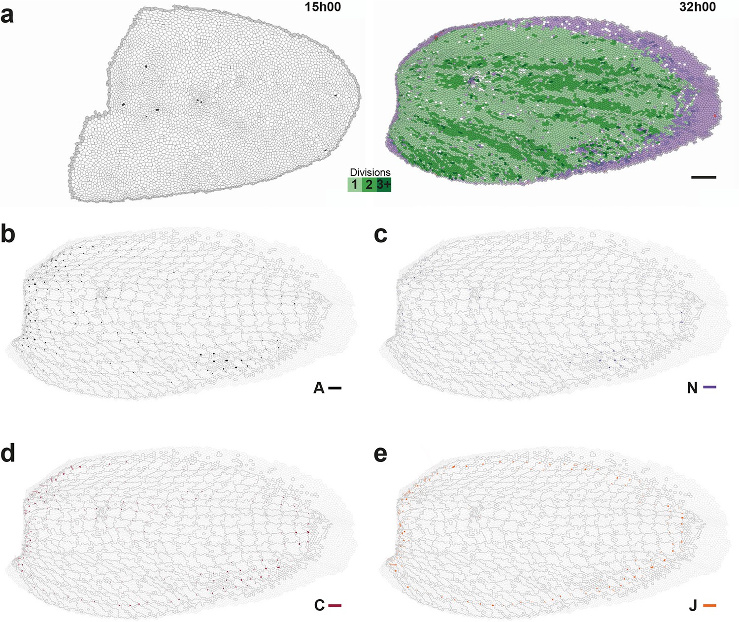
Maps of proliferation and of additional cell process CE rates during wing development.
(a) Rate of cell divisions obtained by cell tracking. Cell divisions at (left) 15 and (right) 32 hAPF; light green cell: one division; medium green cell: two divisions; dark green cells: three divisions and more; purple cells: cells entering the field of view during the movie. (b–e) Average maps of cell process CE rates other than those shown in Figure 5: (b) delaminations , (c) new cell integrations , (d) fusions , (e) boundary flux . Time averages were performed between 15 and 32 hAPF. A local transparency is applied to weight the CE rate according to the number of cells in each group of cells. Scale bars: (a) 50 μm, (b–e) 0.1 h-1.
Figure 6 with 1 supplement
Quantitative characterization of tissue development in trblup mutant notum.
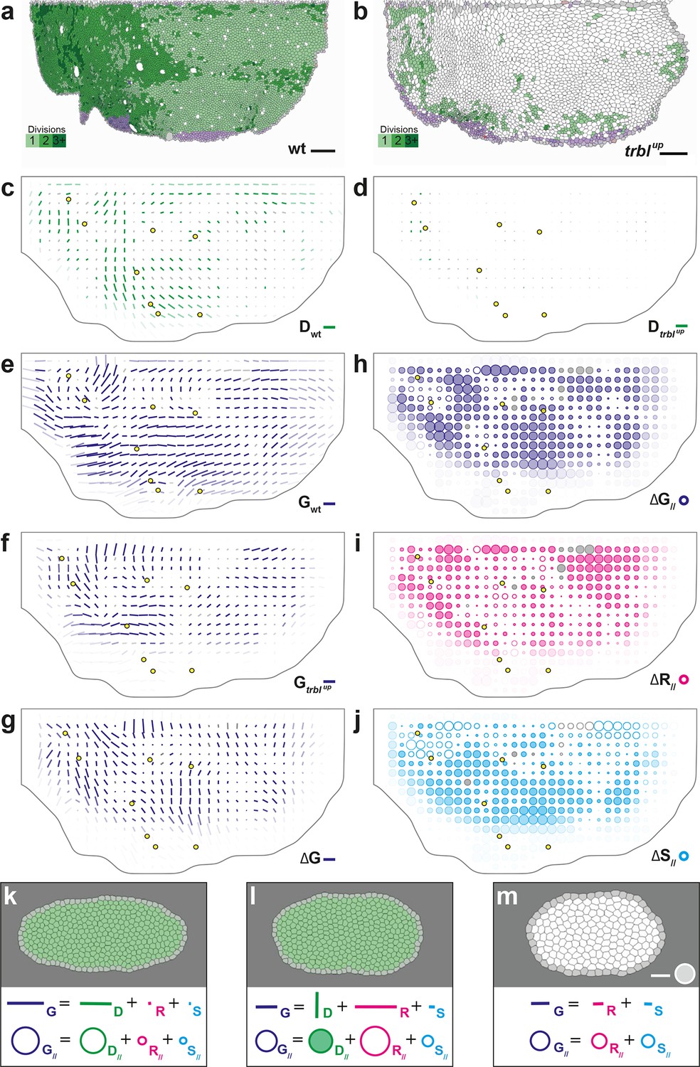
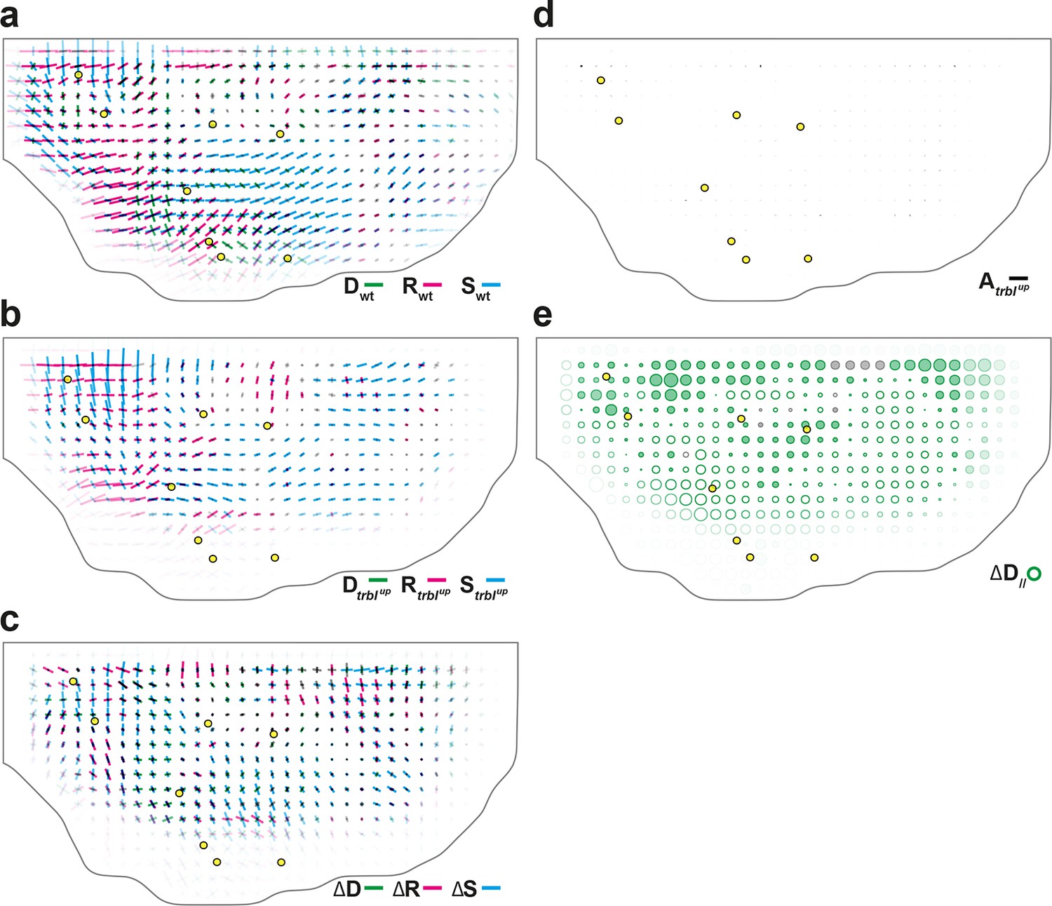
(a,b) Comparison between rate of cell divisions in (a) wild-type (extracted from half of Figure 3c) and (b) trblup tissues. Number of cell divisions color-coded on the last image of the movie (28 hAPF), light green cell: one division; medium green cell: two divisions; dark green cells: three divisions and more; purple cells: cells entering the field of view during the movie. (c–j) Comparisons of CE rates in wild-type and trblup mutant tissues. Time averages were performed between 14 and 28 hAPF. In this Figure (and Figure 6—figure supplement 1), values larger than the local biological variability are plotted in color while smaller ones are shown in grey; a local transparency is applied to weight the CE rate according to the number of cells and hemi-nota in each group of cells; black outline delineates the archetype hemi-notum; the midline is the top boundary; circles filled in yellow indicate archetype macrochaetae. (c,d) Comparison between cell division CE rate (, green) in (c) wild-type (extracted from Figure 4b) and (d) trblup tissues. (e,f) Comparison between tissue CE rate (, dark blue) in (e) wild-type (reproduced from Figure 4a) and (f) trblup tissues. (g–j) Subtraction of measurements in trblup tissue minus measurements in wild-type tissue, for (g) tissue CE rate (, dark blue), and for components along wild-type tissue CE rate of (h) tissue CE rate (, dark blue), (i) cell rearrangements CE rate (, magenta) and (j) cell shape changes CE rate (, cyan). (k–m) Simulations illustrating the impact of cell divisions on tissue elongation and on the other processes. Top: last image of Potts model simulations; bottom: measurement of CE rates (bar) and of their components along (circles). (k) As in Figure 2b, numerically implemented forces elongate the cell patch along the horizontal axis, and cell divisions are oriented along the direction of patch elongation; (l) same as (k) but with divisions now oriented orthogonally to the direction of tissue elongation, and (m) without any division occurring during tissue elongation. Only non-zero values are plotted. Scale bars: (a,b) 50 μm, (c–g) 2 10-2 h-1, (k–m) equivalent to 10-2 h-1 for simulation movies lasting 20 h; scale circle areas: (h–m) 0.1 h-1.
Figure 6—figure supplement 1
Additional quantitative characterizations of trblup tissue development.
(a–c) Maps of overlayed CE rates of cell divisions (, green), cell rearrangements (, magenta) and cell shape changes (, cyan), averaged over 5 hemi-nota, in (a) wild-type tissue (reproduced from Figure 4b for comparison), (b) trblup tissue, (c) their difference. (d) Average map of delamination CE rate (, black) in trblup tissue. Note that the number of delaminations decreased to ~7 102, i.e. 13% of the number of delaminations found in wild-type tissue. (e) Average map of the component along wild-type tissue CE rate of the difference between division CE rate in wild-type and trblup tissues. Time averages were performed between 14 and 28 hAPF. Scale bars: (a–d) 2 10-2 h-1; scale circle area: (e) 0.1 h-1.
Figure 7 with 2 supplements
Maps of junctional stress and comparison with division CE rate .
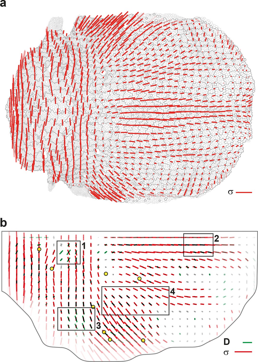
(a) Map of the anisotropic part of local junctional stress covering the whole notum. Average performed between 14 and 28 hAPF, plotted on the last corresponding image: contours of cells (thin grey outlines) and of initially square patches (thick grey outlines). (b) Overlay of division CE rate (, green) and of anisotropic part of junctional stress (, red). Measurements averaged over time between 14 and 28 hAPF and over 5 hemi-nota. In this Figure (and Figure 7—figure supplement 2), values larger than the local biological variability are plotted in color while smaller ones are shown in grey; a local transparency is applied to weight the CE rate according to the number of cells and hemi-nota in each group of cells; black outline delineates the archetype hemi-notum; the midline is the top boundary; circles filled in yellow are archetype macrochaetae. Black rectangular boxes outline the four regions numbered 1 to 4 described in the text, same as in Figure 4. Stress is expressed in arbitrary unit (A.U.) proportional to the average junction tension (not determined by image analysis). Scale bars: (a,b) 0.1 A.U., (b) 2 10-2 h-1.
Figure 7—figure supplement 1

Maps of cell pressures, junction tensions and junctional stress inferred on single images.
Left: 14 hAPF; right: 28hAPF. No averaging over time or animals has been performed on any of these images. (a) Maps of cell pressure , expressed in arbitrary unit proportional to the average junction tension (not determined by image analysis). The bar on the right indicate the color code. Positive or negative values indicate pressures above or below the average pressure. (b) Maps of apical junction tension , expressed in units of the average cell junction tension. The bar on the right indicate the color code. Values larger or smaller than 1 indicate tensions above or below the average tension. (c) Maps of stress obtained from data of pressure, junction tension and cell size. Stress is expressed in arbitrary unit (A.U.) proportional to the average apical junction tension. By convention, the isotropic part is plotted at zero average, so positive values (white circles) and negative values (grey circles) correspond to isotropic parts above or below average. Scale bar (anisotropic part): 0.1 A.U. Scale circle diameter (isotropic part): 0.1 A.U.
Figure 7—figure supplement 2

Comparison of orientations of junctional stress and cell division orientation .
Overlay of division orientation CE rate (, dark green) and junctional stress (, red) anisotropic part. Measurement averaged over time between 14 and 28 hAPF and over 5 hemi-nota. Black rectangular boxes outline the four regions numbered 1 to 4 described in the text, same as in Figures 4 and 7. Alignment coefficient is 0.67 in R1, 0.98 in R2, 0.94 in R3, 0.89 in R4, and 0.87 over the whole tissue. Stress is expressed in arbitrary unit (A.U.) proportional to the average apical junction tension (not determined by image analysis). Scale bars: 0.1 A.U., 2 10-2 h-1.
Videos
Video 1
Workflow of measurements of tissue and cell process CE rates at the patch scale.
(a) Detail of a movie in the scutellum region, tissue labeled with E-Cad:GFP and imaged by multi-position confocal microscopy at a 5 min time resolution, 11:25 to 27:25 hAPF. (b) Cell tracking: cells are colored in shades of green according to their number of divisions: light (1), medium (2), dark (≥3); black for the last five frames before a delamination; red for fused cells. (c) Evolution of cell-cell links: links which appear or disappear are represented with thick straight lines and colored as follows: divisions (green), rearrangements (magenta), delaminations (black), integrations (purple), fusions (red), boundary flux (orange). Conserved links are represented with thin dark blue lines. Links corresponding to four-fold vertices are in lighter colors. Cell contours are indicated by thin grey outlines, patch contours by thick black outlines. (d-h) Maps of dilation rates (circles filled in white [positive] or grey [negative]) and of CE rates (orientation: bar direction; anisotropy: bar length), for (d) the tissue (compare bar amplitudes and orientations with the evolution of patch shapes), (e) cell divisions , (f) rearrangements , (g) cell size and shape changes and (h) delaminations . Patch contours are indicated by thick grey outlines. Dilation and CE rates in a given patch are calculated from the evolution of links in this patch between two successive images, then averaged with a sliding window of 2 h. The stillness at the beginning and end of the measurement movies comes from this time averaging.
Video 2
Movies of computer simulations corresponding to (a-d) Figure 2a–d and to (e–i) Figure 2—figure supplement 1a–e.
(a) Cell size and shape changes , (b) oriented cell divisions , (c) oriented cell rearrangements , (d) delaminations , (e) integrations of new cells , (f) fusions of two or more cells , (g) cell flux , (h) rotation, (i) convergence-extension with initial and final states similar to those in (h).
Video 3
Movies of cell tracking, cell trajectories and patch deformation in the whole Drosophila notum.
(a) Cell tracking displaying divisions (see Figure 3c): cells are color coded in light green for the first division, medium green for two divisions, dark green for three divisions and more; black for the last five frames before a delamination; red for cells that fuse; grey for the first layer of boundary cells; purple for new cells. (b) Cell trajectories: as it moves, each cell leaves a trail corresponding to the successive positions of its center in the last 10 images. Same color code as in (a). (c) Growth and morphogenesis of cell patches during development (see Figure 3d). Cell contours are indicated by thin grey outlines, cells within a patch have same arbitrarily assigned colors that respect the symmetry with respect to the midline. Movie between 11:30 and 30:45 hAPF. Note that the original movie of the E-Cad:GFP tissue is visible in Supplementary Video 1 of (Bosveld et al., 2012).
Video 4
Time evolution of the cell process CE rates and of the anisotropic junctional stress over the whole Drosophila notum.
(a-e) Time evolution of CE rates of (a) tissue morphogenesis , (b) oriented cell divisions , (c) oriented cell rearrangements , (d) cell shape changes , (e) delaminations (see also Figure 3f-j). (f) Time evolution of the anisotropic part of the junctional stress (see also Figure 7). Movie between 14 and 28 hAPF, 2 h sliding window average plotted every 5 min.
Video 5
Growth and morphogenesis during wing development, 15 to 32 hAPF.
(a) Tissue labeled with E-Cad:GFP and imaged by multi-position confocal microscopy at a 5 min time resolution. (b) Growth and morphogenesis of cell patches during development (see Figure 5a). Cell contours are indicated by thin grey outlines, patch contours by arbitrarily assigned colors. (c–f) Time evolution of CE rates of (c) the tissue , (d) oriented cell divisions , (e) oriented cell rearrangements , (f) cell shape changes (see Figure 5b–e).
Video 6
Potts model simulations illustrating the impact of cell divisions on tissue elongation and on the other cell processes (see Figure 6k–m).
(a) As in Figure 2b, numerically implemented forces elongate the cell patch along the horizontal axis, and cell divisions are oriented along the direction of patch elongation. (b) Same as (a) but with divisions now oriented orthogonally to the direction of tissue elongation. (c) Same as (a) but without any division occurring during tissue elongation.
Download links
A two-part list of links to download the article, or parts of the article, in various formats.
Downloads (link to download the article as PDF)
Open citations (links to open the citations from this article in various online reference manager services)
Cite this article (links to download the citations from this article in formats compatible with various reference manager tools)
Unified quantitative characterization of epithelial tissue development
eLife 4:e08519.
https://doi.org/10.7554/eLife.08519


