Mammal communities are larger and more diverse in moderately developed areas

  1. Arielle Waldstein Parsons  Is a corresponding author
  2. Tavis Forrester
  3. Megan C Baker-Whatton
  4. William J McShea
  5. Christopher T Rota
  6. Stephanie G Schuttler
  7. Joshua J Millspaugh
  8. Roland Kays
  1. North Carolina Museum of Natural Sciences, United States
  2. North Carolina State University, United States
  3. Oregon Department of Fish and Wildlife, United States
  4. Smithsonian Conservation Biology Institute, United State
  5. The Nature Conservancy, Virginia
  6. West Virginia University, United States
  7. University of Montana, United States

Abstract

Developed areas are thought to have low species diversity, low animal abundance, few native predators, and thus low resilience and ecological function. Working with citizen scientist volunteers to survey mammals at 1427 sites across two development gradients (wild-rural-exurban-suburban-urban) and four plot types (large forests, small forest fragments, open areas and residential yards) in the eastern US, we show that developed areas actually had significantly higher or statistically similar mammalian occupancy, relative abundance, richness and diversity compared to wild areas. However, although some animals can thrive in suburbia, conservation of wild areas and preservation of green space within cities are needed to protect sensitive species and to give all species the chance to adapt and persist in the Anthropocene.

https://doi.org/10.7554/eLife.38012.001

eLife digest

Humans transform natural ecosystems worldwide into towns and cities, replacing natural habitat with human-built surfaces. This loss of habitat and increase in human activity make suburban areas difficult for some species to survive in, raising concerns that developed areas become ecologically unbalanced as they lose biodiversity. However, the preservation of urban green space and lack of hunting could also open the door for some species to thrive in the midst of large human populations. Indeed, some animals, mammals in particular, have grown more tolerant of humans and appear to have adapted to suburban landscapes around the world. Some species that have been exclusively living in the wilderness, such as a small carnivore called the fisher, are even moving back into cities.

Research into how mammals are coping with the urbanization of their habitats has produced conflicting results. Studies that explore a variety of cities and habitats would help to clear up this confusion.

Parsons et al. worked with citizen scientist volunteers to survey the mammals at 1,427 sites across Washington DC and Raleigh, North Carolina. The volunteers set up motion-triggered cameras in these sites, which covered a full range of urban and wild habitats, including back yards and large nature preserves.

The cameras detected similar or higher numbers of mammal species in suburban sites compared to wild areas. Indeed, most species appear to use suburban areas at least as much as wild land. Urban green space is especially important; it is used by less urban-adapted species like coyotes to navigate areas that are densely populated by humans.

The results presented by Parsons et al. suggest that many mammals have indeed adapted to the suburban environment over the last few decades, resulting in more balanced urban ecosystems. More testing in other cities will help to determine how general this pattern of adaptation is, and provide us with knowledge that could help us to conserve many different species. However, some species were still most abundant in wild areas, emphasizing the need to also conserve wildlands and to minimize our impact on natural ecosystems.

https://doi.org/10.7554/eLife.38012.002

Introduction

Global loss of biodiversity leads to disruption of ecosystem services around the world, ultimately threatening human well-being (Cardinale et al., 2012). Vertebrate species loss is typically considered to be worst in the most developed landscapes, where urbanization serves as an intense and long-term disturbance that permanently alters habitat and truncates food webs (Lombardi et al., 2017; McKinney, 2006). However, for some species, urbanization can offer abundant nutrient-rich food that is less ephemeral compared to wild areas (Bateman and Fleming, 2012; Wang et al., 2017). Whether this food is enough to counteract the negative effects of disturbance (i.e. higher road mortality, fragmentation) depends on a species’ ability to adapt to the stressors of urban living (Witte et al., 1982). Mammal species, especially those with large home ranges, are arguably most at risk from development, leading some to suggest that developed areas have a dearth of predators, and that prey species could benefit by using humans as a shield (Crooks, 2002; Ordeñana et al., 2010). Previous studies have shown cities to be depauperate of bird life, supporting the traditional view that development and biodiversity cannot coexist (Keast, 1995; Strohbach et al., 2014).

However, recent evidence has shown that some mammal species previously thought mal-adapted to urban landscapes (i.e. mountain lion [Puma concolor], fisher [Martes pennanti]) are thriving in them (Bateman and Fleming, 2012; LaPoint et al., 2013), suggesting an evolutionary trend that could be important for conservation in the Anthropocene. Existing research on mammal communities across urbanization gradients has focused on single cities, yielding conflicting results, perhaps due to variation in city structure and characteristics (Lombardi et al., 2017; Saito and Koike, 2013). Given the rapid expansion of urban areas worldwide, and the recent case studies of urban adaptations by wildlife (LaPoint et al., 2013; Riley et al., 2014; Wang et al., 2017), more large-scale studies are needed to evaluate the response of wildlife communities to urban development if we are to understand urban ecology, conservation, and evolution in the Anthropocene.

Here, we present the results of a large-scale mammal survey of two urban-wild gradients. Our objectives were to determine how diversity, richness, detection rate, and occupancy of the mammal community change as a function of human disturbance. We hypothesized that the availability of supplemental food at higher levels of development would positively affect mammalian populations and outweigh the negative effects of disturbance, except for the most sensitive species. Specifically, we predicted that mammalian relative abundance would increase with developmental level but that species richness and diversity would decrease. Furthermore, we predicted that occupancy of the most sensitive species (i.e. large and medium carnivores) would be highest in wild areas both in our study area and around the world.

Materials and methods

Study sites

Request a detailed protocol

Washington, District of Columbia, USA (hereafter DC) is a city of approximately 177 km2 with an estimated human population size of 681,000, thus a density of 3847 people/km2. Our study spanned a 56,023.7 km2 area around the city with a mean of 4.4 houses/km2 and matrix of agriculture (~21.3%) and forest (~54.1%). Raleigh, North Carolina, USA (hereafter Raleigh) is approximately 375 km2 with an estimated human population size of 459,000, thus a density of 1278 people/km2. Our study spanned a 66,640 km2 area around the city with a mean of 17.7 houses/km2 and matrix of agriculture (~24.3%) and forest (~52.3%).

Citizen science camera trap surveys

Request a detailed protocol

From 20122016, 557 trained volunteers deployed 1427 unbaited camera traps across an urban-wild gradient around Raleigh and DC. Each individual camera was considered a 'camera site' and volunteers ran cameras at an average of two sites each. Following Hammer et al. (2004), we used the Silvis housing density dataset with 1km grid cells to define five development levels of the gradient for sampling stratification (excluding open water): urban (>1000 houses/km2), suburban (147.0481000 houses/km2), exurban (12.64147.047 houses/km2), rural (0.5112.63 houses/km2) and wild (<0.5 houses/km2). Within those gradient levels, camera placement was also stratified between residential yards, open areas (>0.001 km2 absent of trees), small forest fragments (1 km2) and large forest fragments (>1 km2Supplementary file 1. Forest fragment size was verified using the 2006 US National Landcover Dataset (NLCD) and Landscape Fragmentation Tool v2.0 (Vogt et al., 2007) in ArcMap (Version 10.1, ESRI, Redlands, CA, USA) which defines forest fragments by size. Yards were not available for sampling in the urban or wild levels of the gradient. Urban areas were not sampled in Raleigh and open areas were not sampled in DC. All adjacent cameras were spaced at least 200 m apart. Camera placement was randomized as much as possible using ArcMap (Version 10.1) to randomly generate points within polygons while following certain rules. For example, we selected sites within forests that volunteers were permitted to access and were within a reasonable hiking distance (i.e. < 11 km hike round trip) with terrain that was not too steep to traverse safely (i.e. <45 degree slope). Within yards, cameras were placed as randomly as possible while avoiding the highest human traffic areas (i.e. walkways, doors, gates and driveways).

No explicit power analysis was used to predetermine sample size. Our sample size goal was 20 spatial replicates (equating to ~420 trap nights), which has been found to maximize precision for estimating detection rate (Kays et al., 2010; Rowcliffe et al., 2008). Camera sites are biological replicates, parallel measurements capturing random biological variation. This study did not include technical replicates.

Volunteers used Reconyx (RC55, PC800, and PC900, Reconyx, Inc. Holmen, WI) and Bushnell (Trophy Cam HD, Bushnell Outdoor Products, Overland Park, KS) camera traps attached to trees at 40 cm above the ground. Cameras were deployed for three weeks and then moved to a new location without returning, with sampling taking place continuously throughout the year. Cameras recorded multiple photographs per trigger, at a rate of 1 frame/s, re-triggering immediately if the animal was still in view. We grouped consecutive photos into on sequence if they were <60 s apart, and used these sequences as independent records, counting animals in the sequence, not individual photos (Parsons et al., 2016). We then collapsed these independent records into daily detection/non-detection for occupancy modeling. Initial species identifications were made by volunteers using customized software (available freely from eMammal.org, source code proprietary) and all were subsequently reviewed for accuracy before being archived at the Smithsonian Digital Repository (McShea et al., 2016).

Diversity 

Request a detailed protocol

We used package iNEXT (Hsieh et al., 2016) in R (Version 3.1.0; R Development Core Team., 2008) via R Studio (RStudio Team, 2015) to calculate Hill numbers (i.e. the effective number of species, incorporating relative abundance and richness) of species richness and Shannon diversity (Chao et al., 2014) between gradient levels (urban-suburban-exurban-rural-wild) and plot types (yard, open, small forest, large forest). iNEXT calculates the Shannon diversity as Hill number q = 1, equal to the exponential of Shannon's entropy index, thus the natural log of those results was used for display purposes. We used detection/non-detection data to compute diversity estimates and the associated 95% confidence intervals via rarefaction, plotting the diversity estimates while accounting for sample size. We fit a curve to diversity estimates between gradient levels using a generalized additive model with a polynomial term.

Model covariates

Request a detailed protocol

We modeled variation in occupancy (ψ) and detection rate using 13 covariates (Supplementary file 2) representing development level, the amount of core forest, small scale forest cover, prey relative abundance and whether hunting was allowed. We added year as a covariate to account for population changes over time. We used the Landscape Fragmentation Tool v2.0 (Vogt et al., 2007) and the NLCD (2006) land use dataset in ArcMap (Version 10.1) to create a landcover layer representing the percent of large core forest (forest patches larger than 1 km2) in a 5 km radius around camera locations which we considered best approximated the home range size of our target species (Bekoff, 1977; Fritzell and Haroldson, 1982; Lariviere and Pasitschniak-Arts, 1996; Lariviere and Walton, 1997). Forest patches did not necessarily fall entirely within the buffer. We considered road density as an additional covariate at the 5 km scale but initial evaluations showed it to be highly correlated with housing density (87.1%) so we chose to eliminate it from the analysis. We used a 100 m radius for small-scale forest cover to best represent small forest patches within suburban neighborhoods (e.g. small vacant lots with trees, greenways). We represented deer and rodent+lagomorph relative abundance using site-specific detection rate (the number of detections divided by the total number of camera-nights). We included an indicator (0/1, no hunting/hunting) to categorize whether a site allowed hunting or not. We modeled detection probability (p) using five covariates (Supplementary file 2). Because both ambient temperature and undergrowth can affect the camera’s ability to detect an animal, we included daily covariates for temperature and NDVI (Moderate Resolution Imaging Land Terra Vegetation Indices 1 km monthly, an average value over the month(s) the camera ran) obtained from Env-DATA (Dodge et al., 2013). To complement NDVI, we also considered site-specific detection distance, a measure of how far away the camera was able to detect a human, which is influenced by both understory and site topography. We included an indicator (0/1, not yard/yard) to categorize whether a site was a residential yard or not. In Raleigh, two different camera models were used (both Reconyx and Bushnell) so we added a 0/1 (Bushnell/Reconyx) covariate to account for potential difference in detection probability between the two brands. We diagnosed univariate correlations between covariates using a Pearson correlation matrix, and used a restrictive prior for beta coefficients where correlation was >0.60 (i.e. logistic(0,1); a prior with reduced variance to induce shrinkage, similar to ridge regression; Hooten and Hobbs, 2015). All covariates were mean-centered.

Detection rate models 

Request a detailed protocol

We used a Poisson count model (e.g. Kays et al., 2017) to assess differences in total mammal detection rate (i.e. the intensity with which a site was used, count/day) between the five gradient levels (urban, suburban, exurban, rural, wild) and four plot types (large forest, small forest, open, yard). We fit a curve to total detection rate estimates between gradient levels using a generalized additive model. No other covariates were used in this model. We then ran separate count models for four predator species (coyote (Canis latrans), gray fox (Urocyon cinereoargenteus), red fox (Vulpes vulpes) and bobcat [Lynx rufus]) to evaluate covariates of detection rate, running one fully-parameterized model (Supplementary file 2) to evaluate which explained the most variation in detection rate. We assessed model fit with posterior predictive checks (PPC) (Gelman et al., 2014; Kery and Schaub, 2012) by calculating the sum of squared Pearson residuals from observed data (T(y)) and from data simulated assuming the fully parameterized model was the data-generating model (T(ysim)). We calculated a Bayesian p-value as pB = Pr(T(ysim)>T(y)) from posterior simulations and assumed adequate fit if 0.1 < pB < 0.9 (Supplementary file 3). We fit the detection rate model in OpenBUGS v3.2.3 (Lunn et al., 2009) via R2OpenBUGS v3.2 (Sturtz et al., 2005) in R (Version 3.1.0) via R Studio. We based inference on posterior samples generated from three Markov chains, using trace plots to determine an adequate burn-in phase. All models achieved adequate convergence (R^≤1.1) (Gelman et al., 2014) by running for 50,000 iterations following a burn-in phase of 1000 iterations, thinning every 10 iterations. We based significance on whether parameter 95% credible intervals overlapped zero.

Occupancy models 

Request a detailed protocol

We used the multispecies occupancy model of Rota et al. (2016) to estimate the probability of occupancy of four predator species: bobcat, coyote, red fox and gray fox. Although we are using the term occupancy, because data were collected from camera traps estimates are more analogous to ‘use’ than true occupancy (Burton et al., 2015). This model is distinct from the classic multispecies community models (Dorazio and Royle, 2005;Dorazio et al., 2006; Gelfand et al., 2005) and is rather a generalization of the single-season occupancy model (MacKenzie et al., 2002) to accommodate two or more interacting species. It contains single-species (first order) occupancy models for each interacting species alone as well as pairwise (second order) models for the co-occurrence of each pair of species (Rota et al., 2016). For each species and pairwise interaction, the model estimates detection probability (p), defined as the probability of detecting an occurring species at a camera site, and occupancy (ψ), defined as the probability that a given camera site is occupied, for each species. The latent occupancy state of each species at a site is modeled as a multivariate Bernoulli random variable such that (assuming 2 interacting species):

Z~MVB(ψ11, ψ10, ψ01, ψ00)

Where ψ11is the probability that both species occupy a site, ψ10 is the probability that only species 1 occupies a site, ψ01 is the probability that only species 2 occupies a site and ψ00 is the probability that neither species occupies a site. We assumed all species occurred independently and considered the same set of five covariates for the detection probability models and 13 covariates in the occupancy model of each species (Supplementary file 2). We considered interactions (i.e. city*covariate) between each occupancy covariate and city (0/1, DC/Raleigh). We estimated occupancy for each species across levels of the development gradient (urban, suburban, exurban, rural, wild) and plot types (yard, open, small forest, large forest) within each city separately by including development level and plot type as categorical covariates in our model.

We fit models in STAN (Version 2.15.1; Stan Development Team, 2015b) via the RSTAN (Version 2.15.1; Stan Development Team, 2015a) interface in R (Version 3.4.0) via R Studio (Version 1.0.143). We based inference on posterior samples generated from two Markov chains, using trace plots to determine an adequate burn-in phase and subsequently running chains until they reached adequate convergence (R^>1.1) (Gelman et al., 2014). All models achieved adequate convergence by running for 3000 iterations following a burn-in phase of 1000 iterations. We based predictor significance on whether beta coefficient 95% credible intervals overlapped zero. We assessed model fit with posterior predictive checks (PPC) (Gelman et al., 2014; Kery and Schaub, 2012) by calculating the sum of squared Pearson residuals from observed data (T(y)) and from data simulated assuming the fully parameterized model was the data-generating model (T(ysim)). We calculated a Bayesian p-value as pB = Pr(T(ysim)>T(y)) from posterior simulations and assumed adequate fit if 0.1 < pB < 0.9. To our knowledge, the squared Pearson’s residual has not been derived in the context of occupancy models, so we present our derivation of this test statistic in Supplementary file 4. We added a random effect on detection/non-detection for the coyote portion of the model since initial assessments of fit for this species were inadequate (i.e. pB >0.9). We assessed differences in occupancy between gradient levels for each species using overlapping 95% confidence intervals.

Comparison with global occupancy data 

Request a detailed protocol

We removed omnivores from the dataset of Rich et al. (2017) to better compare with carnivore occupancy from our own dataset. Where species occupancy was estimated from multiple studies in the Rich et al. dataset, we calculated averages to compare to occupancy estimates from our own study. We summarized occupancy estimates of Rich et al. and our own study within each developmental level using a box and whisker plot and assessed statistically significant differences based on whether or not interquartile ranges overlapped.

Data accessibility

Request a detailed protocol

Raw detections data have been deposited in Data Dryad, doi:10.5061/dryad.11rf64v. The software used for initial species identifications is available via eMammal.org. To download and use the software, users must first create an account on eMammal and become associated with an existing project. This can be done by using the 'Join' button on the project's homepage, or by emailing the contact person, also listed on the project homepage. Usually the user will also have to pass an online or in person training, depending on the project requirements, to be approved to download the software.

Results and discussion

Working with citizen scientist volunteers, we obtained 53,273 detections of 19 mammal species at 1427 sites along an urban-wild gradient in Washington, DC and Raleigh, NC, USA, sampling both private and public lands. In DC, we detected 17 mammal species with mean naïve occupancy of 0.19 (min = 0, max = 0.93) and mean detection rate of 0.09 detections/day (min = 0, max = 1.05). In Raleigh, we detected 17 mammal species with mean naïve occupancy of 0.14 (min = 0, max = 0.79) and mean detection rate of 0.08 detections/day (min = 0, max = 0.09).

We found no significant decline of species diversity or richness from suburban to wild gradient levels (Figure 2—figure supplement 1, Figure 1). However, Shannon diversity was significantly lower at the urban level in DC, possibly due to low sampling (Figure 2, Supplementary file 1). Diversity in yards was significantly higher or not statistically different from large and small forest fragments in both cities (Figure 2—figure supplements 2,3). Most (92.3%) of the 13 mammal species detected >20 times occupied all levels of development below the urban level. Two of the largest predators, coyotes and bobcats, were absent from the highest development level (urban) but were detected at all other levels in both cities. Black bears (Ursus americanus), which are actively discouraged from colonizing central North Carolina (North Carolina Wildlife Resources Commission, 2011), were not detected in Raleigh and were detected in DC at all levels of the gradient except suburban and urban, though were predominantly in the wild level. These results indicate that the extant mammal guild exploits all levels of the urban-wild gradient and that no species are entirely relegated to the wild gradient level. However, some species appear less adapted to habitation in human-dominated areas, spending most of their time at the wild levels of the gradient (i.e. bobcat, bear; Figure 1). We recognize that the current community represents species that survived the initial arrival of high-density human settlement. In particular, two large predators (wolves (Canis lupus) and cougars [Puma concolor]) were extirpated from our study area a century ago. However, even cougars and wolves have recently shown surprising adaptability in the face of development at other sites (Bateman and Fleming, 2012; Wang et al., 2017) suggesting that, given enough time and protection from persecution, many of the most ‘wild’ of species may adapt to human development.

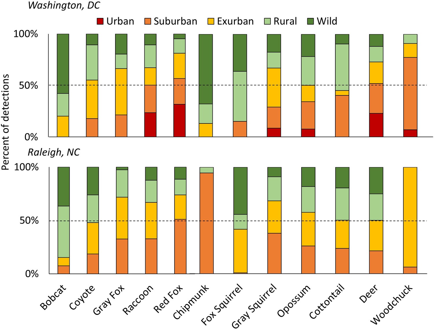
The percent of detections for each species of carnivores (left) and herbivores (right) in each development level along the urban-wild gradient in Washington, DC and Raleigh, NC, USA accounting for the effort (i.e. camera nights) within each level, sorted from lowest to highest proportion urban/suburban in DC.

The dashed line shows 50% of total detections. Some species were predominantly rural/wild (i.e. bobcats and fox squirrels) while others were mainly detected in urban/suburban habitats (i.e. red fox, raccoon). Patchy distributions at different gradient levels were seen for species at the edge of their ranges (i.e. chipmunks and woodchucks in Raleigh). Urban habitats were not sampled in Raleigh.

https://doi.org/10.7554/eLife.38012.003
Figure 2 with 3 supplements see all
Mean Shannon diversity and total detection rate along a gradient of housing density in two cities, Washington, DC and Raleigh, NC USA taken from camera traps.

Bars show 95% confidence intervals, lines are fit using a generalized additive model with a polynomial term. Diversity peaked at intermediate levels of urbanization (exurban in DC and suburban in Raleigh). Total detection rate peaked at the urban level in DC and exurban level in Raleigh.

https://doi.org/10.7554/eLife.38012.004

Predators are thought to be the most at risk from urbanization (Crooks, 2002), therefore, we evaluated predictors for occupancy (MacKenzie et al., 2002) and detection rate (Kays et al., 2017) for four carnivores: coyote, gray fox, red fox, and bobcat. Both of our models fit well, with Bayesian p-values between 0.1 and 0.9 (Supplementary file 3). Suburban and urban occupancy probabilities were not statistically different from wild for any of the species (Figure 3—figure supplement 1) and we noted a decreasing trend in occupancy from urban to wild (Figure 3). We compared the occupancy estimates from our study to those reported for carnivores in protected areas around the world (Rich et al., 2017) and found no significant difference (Figure 3), suggesting that the ecological function of predators in this urban system is not substantially reduced from the current wild state, excepting the historical extirpation of the two largest native predators from the region.

Figure 3 with 1 supplement see all
Comparison of carnivore (i.e.bobcat, coyote, gray fox, red fox) occupancy probabilities at each developmental level in two cities with global values from Rich et al.

(Rich et al., 2017), representing 93 carnivores from 13 protected areas on five continents (Global Wildlands). Each box for our dataset represents the distribution of marginal occupancy probabilities for each of four carnivore species in that city (i.e. four probabilities). The boxes for Global Wildlands represent the distribution of marginal occupancy probabilities for 93 species. We found no statistically significant differences between any habitat levels in our study or between our study and global wildland occupancy probabilities but noted a decreasing trend in occupancy from urban-wild. We included only predators from Rich et al. (2017) and removed omnivores (i.e. raccoon, coati) to better reflect our data.

https://doi.org/10.7554/eLife.38012.008

Our occupancy and detection rate models yielded similar results (Supplementary file 57) demonstrating that green space is important to carnivore species that are less-adapted to human-altered landscapes. These models show a greater association of carnivores with green space when housing density is high (e.g. coyote and gray fox, Supplementary file 6, 7), consistent with other studies finding urban green space important in maintaining biodiversity in cities (Gallo et al., 2017; Lombardi et al., 2017; Matthies et al., 2017). It is likely that shyer species are not avoiding regions of high human density, but require patches of forest to navigate residential areas that are freely used by more commensal species, such as red foxes (Tigas et al., 2002), which we frequently detected in yards. Indeed, we found a gradient of responses in carnivore use of human-dominated environments, from red fox which are the most urban adapted (i.e. negatively associated with local large forest fragments and the only species to have a positive association with yards) to bobcats which appear to be the most human-averse (i.e. rarely detected in the suburban level of the gradient) (Figure 1; Figure 3—figure supplement 1).

Contrary to expectations, we found no evidence for a negative impact of suburban and exurban development on extant native mammal diversity, richness, and occupancy and detection rate of carnivores. In fact, all metrics were significantly greater than, or equal to, wild areas. We suspect that developed areas offer good food resources for wildlife through direct and indirect feeding (i.e. bird feeders supplementing prey, pets), accidental feeding (i.e. garbage), and ornamental plantings (for herbivores), but testing this hypothesis will require additional diet studies in urban landscapes (Contesse et al., 2004). Furthermore, the structure of mature suburbia (i.e. older, established neighborhoods with large trees, wooded riparian areas, small parks) contributes to a more diverse and varied landscape than wild areas with more homogenous forest cover, which is potentially beneficial for many generalist species. Developed areas where hunting is limited or prohibited also offer a safe haven for game species, presuming they can navigate the road networks (Collins and Kays, 2011) and avoid direct human conflict.

Our discovery of a wild suburbia suggests high levels of adaptation by mammals to developed landscapes over the last few decades, including predators and prey. The resilience of these species gives hope for wildlife in the Anthropocene, but the generality of this pattern needs to be tested in other cities to understand how habitat type, development patterns, apex predators, and hunting regulations influence urban mammal communities, as there are examples of far more drastic impacts of urbanization on other taxa and in other places around the globe (Keast, 1995; McKinney, 2008). Indeed, in Tokyo, Japan, the relative abundance of mammals declined with urbanization (Saito and Koike, 2013) and avian communities in Quebec, Canada and Rennes, France showed a similar decline in richness (Clergeau et al., 1998; Saito and Koike, 2013). This suggests that city structure, size and human density may influence mammalian distribution along urban-wild gradients with large, sprawling New World cities showing different patterns than the smaller more concentrated cities of the Old World. Although our study provides a less dire picture of urban ecosystem function than previously thought, we do not suggest abandoning mitigation of urbanization’s negative impacts, or conservation of completely wild areas. Factors such as urban green space, connectivity and availability of completely wild areas give species the time and space to adapt to changing habitats and climates. Further understanding of how urban wildlife navigates human-dominated areas and factors that contribute to the adaptation of species to the Anthropocene will be critical to maintaining diversity in a rapidly urbanizing world.

Data availability

Raw detections data have been deposited in Data Dryad, doi:10.5061/dryad.11rf64v. The software used for initial species identification is available via eMammal.org. To download and use the software, users must first create an account on eMammal and become associated with an existing project. This can be done by using the 'Join' button on the project's homepage, or by emailing the contact person, also listed on the project homepage. Usually the user will also have to pass an online or in person training, depending on the project requirements, and they will then become approved to download the software.

The following data sets were generated

References

  1. Book
    1. Gelman A
    2. Carlin JB
    3. Stern HS
    4. Dunson DB
    5. Vehtari A
    6. Rubin DB
    (2014)
    Bayesian Data Analysis (Third edition)
    CRC Press.
  2. Software
    1. Hsieh TC
    2. Ma KH
    3. Chao A
    (2016)
    iNEXT: iNterpolation and EXTrapolation for Species Diversity , version (Version 2.0.12)
    iNEXT: iNterpolation and EXTrapolation for Species Diversity .
    1. Kays R
    2. Tilak S
    3. Kranstauber B
    4. Jansen PA
    5. Carbone C
    6. Rowcliffe MJ
    7. He Z
    (2010)
    Monitoring wild animal communities with arrays of motion sensitive Camera traps
    arXiv.
  3. Book
    1. Kery M
    2. Schaub M
    (2012)
    Bayesian Population Analysis Using Win-BUGS: A Hierarchical Perspective
    Waltham: Academic Press.
  4. Book
    1. Kéry M
    2. Royle JA
    (2015)
    Applied Hierarchical Modeling in Ecology: Analysis of Distribution, Abundance and Species Richness in R and BUGS: Volume 1: Prelude and Static Models
    Amsterdam: Academic Press.
    1. North Carolina Wildlife Resources Commission
    (2011)
    North Carolina Black Bear Managementplan 2012-2022
    North Carolina Black Bear Managementplan 2012-2022.
  5. Software
    1. R Development Core Team.
    (2008)
    R: A language and environment for statistical computing, version 3.4.0
    R Foundation for Statistical Computing, Vienna, Austria.
  6. Software
    1. RStudio Team
    (2015)
    RStudio: Integrated Development for R, version 1.0.143
    RStudio, Inc, Boston.
    1. Stan Development Team
    (2015)
    Stan: a C++ library for probability and sampling
    Stan: a C++ library for probability and sampling.
    1. Sturtz S
    2. Ligges U
    3. Gelman A
    (2005)
    R2WinBUGS: a package for running WinBUGS from R
    Journal of Statistical Software 12:1–16.
    1. Stan Development Team
    (2015)
    Rstan: the R interface to Stan
    Rstan: the R interface to Stan.
    1. Witte R
    2. Diesing D
    3. Godde M
    (1982)
    Urbanophobe, urbanoneutral, urbanophile – behavior of species concerning the urban habitat
    Flora : The Journal of Infectious Diseses and Clinical Microbiology = Infeksiyon Hastalıkları Ve Klinik Mikrobiyoloji Dergisi 177:265–282.

Decision letter

  1. Bernhard Schmid
    Reviewing Editor; University of Zurich, Switzerland
  2. Ian T Baldwin
    Senior Editor; Max Planck Institute for Chemical Ecology, Germany
  3. Bernhard Schmid
    Reviewer; University of Zurich, Switzerland
  4. Marc Kéry
    Reviewer
  5. Ingolf Kühn
    Reviewer

In the interests of transparency, eLife includes the editorial decision letter and accompanying author responses. A lightly edited version of the letter sent to the authors after peer review is shown, indicating the most substantive concerns; minor comments are not usually included.

Thank you for submitting your article "Wild suburbia: mammal communities are larger and more diverse in moderately developed areas" for consideration by eLife. Your article has been reviewed by four peer reviewers, including Bernhard Schmid as the Reviewing Editor and Reviewer #1, and the evaluation has been overseen by Ian Baldwin as the Senior Editor. The following individuals involved in review of your submission have agreed to reveal their identity: Marc Kéry (Reviewer #3) and Ingolf Kühn (Reviewer #4).

The reviewers have discussed the reviews with one another and the Reviewing Editor has drafted this decision to help you prepare a revised submission.

Summary:

The value of this paper is that it addresses a question of broad relevance with novel methods. The question is whether human population density near two US cities reduces the occurrence of large mammals in four types of habitats, large forests, forest fragments, open areas and yards. The assessment method involved 557 citizens operating cameras deployed for around 20 days at each of 1427 locations throughout a period of 4 years. In addition, the authors compared the results of this assessment with a global data set.

The result was that mammal occurrence did not decline with human population density and even showed an opposite tendency, except for bobcats. Even though this results is not "strong" in the sense that the main point is the absence of a negative influence of human population density, it does send a very important message, in particular because it is based on such a large sampling scheme with a clear design of five human population density levels (wild < rural < exurban < suburban < urban) factorially crossed with the four habitat types (obviously, these two factors were not fully orthogonal because for example open areas and yards could not be found in the wild).

Essential revisions:

The interpretation of human population density as equivalent to disturbance is less important than implied by the authors and should be better justified. In particular, the comparison with the so-called intermediate disturbance hypothesis at the start of the Results and Discussion section seems unnecessary and unjustified, because it is not really tested later on nor even discussed. In fact, the curves drawn in Figure 1 are not really hump-shaped and probably do not have significant downwards curvature at high human population density (interpreted as high disturbance). The hump is even more elusive if Figure 3 is inspected.

Currently, the discussion is somewhat US-centered. Although the two case-study cities are from that region, it would make the paper more relevant if comparisons with literature from other regions, including Europe, and involving other taxonomic groups would be included. In this context it would also be important to put the levels of human population densities in the two studied cities in relation to cities in the old world, which often occupy much smaller areas.

The major issue you need to address in the revision is the description of methods. The detailed comments from the reviewers in this regard are listed below:

I am not sure whether the results are influenced by a measurement bias, i.e. species tending to have higher activity in more disturbed regions and hence being more frequently recorded.

Subsection “Detection rate models”: Either refer from here to the last paragraph of the “Occupancy models” subsection or mention already here how large (long) the burn-in phase was and report the value of i.

Subsection “Occupancy models”: To me it is not clear which species were paired: all ones, or just predators?

Subsection “Occupancy models”: Explain the elements of the formula (including subscripts).

Subsection “Comparison with global occupancy data”: Be explicit on how this was assessed.

Currently, the information about the study design is placed in different parts of the manuscript so that it is difficult to get the overview. Supplementary file 1 is the most useful in this context, even though it would be easier if number of camera locations would also be shown (in addition to number of nights). It is not clear, if there was an additional spatial stratification that was not used in the analyses. For example, I could imagine that within each cell in Supplementary file 1 there were some spatial units and within these spatial units camera locations. Even if that was not the case, the question remains if spatial distance and arrangement of camera locations should have been considered.

Why did you use the crude models of rarefaction rather than obtain the inferences on species richness (including species accumulation) from the multi-species occupancy model of Rota et al.? See Dorazio et al. (2006) for how this can be done. Also, please cite the important work of Dorazio and Royle (2005) and Dorazio et al. (2006) as a foundation on which models such as that by Rota et al. are built.

- Subsection “Model covariates” the sentence “We represented whether a site allowed hunting or not using 0/1.” sounds strange, rewrite.

- Subsection “Model covariates”: Please explain what a restrictive prior is.

- Subsection “Occupancy models”: Really, the other basic groundstone on which your work is based are the multispecies occupancy models of Dorazio and Royle and of Gelfand (independently developed in 2005). These should also be cited.

- Subsection “Occupancy models”: “We assumed all species occurred independently…”. Does this fit with what was just said “It contains single-species (first order)…”?

Subsection “Data reporting”: The first part of this paragraph is a bit weird to me. If you have to have a formal paragraph like this for the journal specifications, please ignore. As of now it reads like you are trying to convince the reader why an observational study was chosen instead of a true experiment. I think it is given that a camera trap study is going to be more of an observational study – we just try to standardize our sampling design as much as possible. If this paragraph is not required, I would just go straight into your methods – i.e. study design, site selection, sample size, etc.

Subsection “Data reporting”: How did you randomize your sites? Did you use GIS and place random points within some bounds of a polygon (e.g. yard or forest preserve)? Did you place a grid across the city and chose sites closes to a random intersect? Please be more specific.

Subsection “Citizen science camera trap surveys”: Please report the mean number of cameras deployed per volunteer (as an aside, please be consistent with the use of volunteer and citizen scientist).

Subsection “Citizen science camera trap surveys”: 200 m seems close together for mammal occupancy. Please justify the independence between sites, or, consider changing your terminology from true occupancy and maybe use habitat use instead.

Subsection “Citizen science camera trap surveys”: Were cameras rotated continuously throughout the year or did sampling only occur during a particular season. Please clarify? If they were rotated throughout the year, did you revisit sites or are some sites sampled in the earlier part of the calendar year being compared to sites sample later (let’s say early spring vs. late fall). If this is the case I would be worried that the sampling periods would violate the assumption of closure for your occupancy models. Please clarify and or address the issue.

Throughout the statistical analyses: It is clear that multiple authors wrote the different sections. Please take the time to be consistent in your tone, terminology, and methods descriptions throughout. For, example R is cited 3 different ways.

Subsection “Model covariates”: Please justify why you decided to use a single season occupancy model for multiple seasons with a year covariate instead of a dynamic occupancy model. The way you did it is not wrong but does not consider the dynamics between years. If you are violating closer (see comment above), you could sub-divide your data into appropriate seasons (considering closure) and use a multi-season occupancy model instead.

Subsection “Model covariates”: Please specify if you used NLCD land use data set and used an open space category or used the NLCD canopy cover dataset.

Subsection “Model covariates”: I am a bit confused here. So, you used the percentage of forested area within the 5 km buffer that was at least connected to a large continuous forest patch larger than 1km? Could that linkage continue outside the patch? For example, would a small 5m2 patch on the edge of the buffer be counted if it were connected to a larger forest patch that continues outside the buffer? It’s just a bit confusing, please clarify.

Subsection “Model covariates”: Also confused here. So now you measured the percentage of forest cover within a 100m radius? But it didn't have to be connected to continuous forest cover? So, a small vacant lot with some trees would be counted?

Subsection “Model covariates”: I have concerns about using number of detections/trap night as a metric of prey abundance (even just relative abundance). In our system, we get rabbits just sitting in front of the camera all day. How can you tease apart that a single rabbit didn't sit in front of the camera continuously triggering it at one site, but not another. For example, what if in a single night one rabbit sat in front of a camera for 100 minutes (100 detections) at site A and 100 rabbits passed in front of the camera a single time (100 detections) at site B? Very different abundance, but you get the same answer.

Subsection “Model covariates”: Does NDVI get at understory? Will a cell with really dense canopy cover but no understory give a different value than one with really dense canopy cover and thick understory? From what I have experienced, dense canopy cover in an urban park (with no understory) will often show up the same as a forested area if there are few gaps in the tree.

Subsection “Model covariates”: Did you use monthly NDVI, did you pick a month with peak greenness, or did you average across the month? I am assuming you used one value since you did not use a dynamic occupancy model, but please clarify.

Subsection “Model covariates”: Indicate which camera model was the reference.

Subsection “Detection rate models”: Did you have adequate fit for both your Poisson and occupancy models? Figure 4—figure supplement 1 has huge error bars, which could be a result of over parameterizing the model. Maybe report results from PPC in supplemental table. However, PPC checks for occupancy models are tough as they have trouble accounting for the correcting of detection. Cross validation is probably best. See Hooten and Hobbs (2015).

Subsection “Occupancy models”: I think you need to mention that you ran an occupancy model for a subset of species (and mention species) somewhere here. Unless you ran a multi-species model for all the species, in which case I don't see any mention of the rest of the species in the Results section.

Subsection “Occupancy models”: I am assuming that the city indicator is a 1 or a 0 based on your table in supplemental material, but this is not clear in the text. Please clarify how that interaction is formulated. You also need to report which city is represented by 1 and which city is represented by 0. Without this your tables don't mean much. You also need to report the intercept value of your model in your supplemental tables, so the reader can interpret results for the reference city.

Subsection “Comparison with global occupancy data”: Here is where the global comparison is first mentioned. I think you need a justification and a bit of a background in the introduction. Until I got to the Discussion section and saw the results, I was left wondering what the point of this analysis was.

Subsection “Study sites”: This passage is written a bit unclearly. As is, it sounds like you deliberately avoided urban areas in both cities. I suggest rephrasing for clarity.

Subsection “Model covariates”: I am assuming 'hunting' means hunting was allowed or hunting was recorded during the sample period? Be more specific.

Subsection “Model covariates”: I suggest putting the covariate abbreviation that you use in your models and tables in parentheses after each time they are mentioned in the text. I think this will help the reader follow along.

Subsection “Model covariates”: I suggest rephrasing to "We included an indicator (0 or 1) to categorize whether a site allowed hunting or not." Also, I assume that 0 indicates no hunting? But please be explicit in the text.

Subsection “Detection rate models”: Change 'count' to Poisson.

Subsection “Detection rate models”: I think you should say what your thinning rate was instead of just ith.

Subsection “Occupancy models”: What about plot type and all the other covariates?

https://doi.org/10.7554/eLife.38012.021

Author response

Summary:

The value of this paper is that it addresses a question of broad relevance with novel methods. The question is whether human population density near two US cities reduces the occurrence of large mammals in four types of habitats, large forests, forest fragments, open areas and yards. The assessment method involved 557 citizens operating cameras deployed for around 20 days at each of 1427 locations throughout a period of 4 years. In addition, the authors compared the results of this assessment with a global data set.

The result was that mammal occurrence did not decline with human population density and even showed an opposite tendency, except for bobcats. Even though this results is not "strong" in the sense that the main point is the absence of a negative influence of human population density, it does send a very important message, in particular because it is based on such a large sampling scheme with a clear design of five human population density levels (wild < rural < exurban < suburban < urban) factorially crossed with the four habitat types (obviously, these two factors were not fully orthogonal because for example open areas and yards could not be found in the wild).

Essential revisions:

The interpretation of human population density as equivalent to disturbance is less important than implied by the authors and should be better justified. In particular, the comparison with the so-called intermediate disturbance hypothesis at the start of the Results and Discussion section seems unnecessary and unjustified, because it is not really tested later on nor even discussed. In fact, the curves drawn in Figure 1 are not really hump-shaped and probably do not have significant downwards curvature at high human population density (interpreted as high disturbance). The hump is even more elusive if Figure 3 is inspected.

We have removed the mention of IDH.

Currently, the discussion is somewhat US-centered. Although the two case-study cities are from that region, it would make the paper more relevant if comparisons with literature from other regions, including Europe, and involving other taxonomic groups would be included. In this context it would also be important to put the levels of human population densities in the two studied cities in relation to cities in the old world, which often occupy much smaller areas.

We have attempted to make comparisons with other cities around the world and added one example of other taxa (Results and Discussion section): “Our discovery of a wild suburbia suggests high levels of adaptation by mammals to developed landscapes over the last few decades, including predators and prey. […] Further understanding of how urban wildlife navigates human-dominated areas and factors that contribute to the adaptation of species to the Anthropocene will be critical to maintaining diversity in a rapidly urbanizing world.”

We hesitate to add too much on other taxa to the discussion for the sake of brevity and because the data we collected are relevant to mammals. The body of literature on other taxa (in particular birds and plants) is rich and we feel that further detailed discussion of those studies is not warranted here. However, if the editor feels strongly we will add a more in-depth discussion to that point.

The major issue you need to address in the revision is the description of methods. The detailed comments from the reviewers in this regard are listed below:

I am not sure whether the results are influenced by a measurement bias, i.e. species tending to have higher activity in more disturbed regions and hence being more frequently recorded.

We would argue that higher activity indicates higher use of a particular habitat which is exactly what we are trying to show. We make no claims to density or absolute abundance, which would indeed be tricky due to differences in activity between gradient levels. What we are measuring (with occupancy and relative abundance) is essentially relative use between gradient levels, arguably a habitat preference.

Subsection “Detection rate models”: Either refer from here to the last paragraph of the “Occupancy models” subsection or mention already here how large (long) the burn-in phase was and report the value of i.

We have added this information and simplified the presentation “We based inference on posterior samples generated from three Markov chains, using trace plots to determine an adequate burn-in phase. All models achieved adequate convergence (R^1.1) (Gelman et al., 2014) by running for 50,000 iterations following a burn-in phase of 1000 iterations, thinning every 10 iterations.”

Subsection “Occupancy models”: To me it is not clear which species were paired: all ones, or just predators?

We have clarified this “We used the multispecies occupancy model of Rota et al., (2016), a generalization of the single-season occupancy model (MacKenzie et al., 2002) to accommodate two or more interacting species, to model the occupancy of four predator species: bobcat, coyote, red fox and gray fox.”

Subsection “Occupancy models”: Explain the elements of the formula (including subscripts).

We have added “Whereψ11 is the probability that both species occupy a site, ψ10 is the probability that only species 1 occupies a site,ψ01 is the probability that only species 2 occupies a site and ψ00 is the probability that neither species occupies a site.”

Subsection “Comparison with global occupancy data”: Be explicit on how this was assessed.

We have added clarification to this point “We summarized occupancy estimates of Rich et al. and our own study within each developmental level using a box and whisker plot and assessed statistically significant differences based on whether or not interquartile ranges overlapped.”

Currently, the information about the study design is placed in different parts of the manuscript so that it is difficult to get the overview. Supplementary file 1 is the most useful in this context, even though it would be easier if number of camera locations would also be shown (in addition to number of nights). It is not clear, if there was an additional spatial stratification that was not used in the analyses. For example, I could imagine that within each cell in Supplementary file 1 there were some spatial units and within these spatial units camera locations. Even if that was not the case, the question remains if spatial distance and arrangement of camera locations should have been considered.

Spatial replicates are indeed included in Supplementary file 1, in parentheses next to the camera nights. We also set a minimum spatial distance as part of our design (subsection “Citizen science camera trap surveys”) “All adjacent cameras were spaced at least 200m apart”.

Why did you use the crude models of rarefaction rather than obtain the inferences on species richness (including species accumulation) from the multi-species occupancy model of Rota et al.? See Dorazio et al. (2006) for how this can be done. Also, please cite the important work of Dorazio and Royle (2005) and Dorazio et al. (2006) as a the foundation on which models such as that by Rota et al. are built.

We suspect that the term “multispecies model” is a source of confusion. The “multispecies” model of Rota et al. is not a community model in the sense of Dorazio et al. (2006) and Dorazio and Royle (2005), but rather an extension of the single-species, single-season occupancy models of Mackenzie et al. (2002) and co-occurrence models of Richmond et al. 2010, with no community-level attribute estimators or focus, no species-level effects. We have clarified this in the Materials and methods section: “We used the multispecies occupancy model of Rota et al. (2016) to model the occupancy of four predator species: bobcat, coyote, red fox and gray fox. This model is distinct from the classic multispecies community models (Dorazio and Royle, 2005; Dorazio et al., 2006; Gelfand et al., 2005) and is rather a generalization of the single-season occupancy model (MacKenzie et al., 2002) to accommodate two or more interacting species.”

While we could formulate the model in a similar way to Dorazio/Royle community models, adding hyperparameters for richness, we think the rarefaction estimates are adequate for the story we are telling.

- Subsection “Model covariates” the sentence “We represented whether a site allowed hunting or not using 0/1.” sounds strange, rewrite.

We have changed this to “We included an indicator (0/1, no hunting/hunting) to categorize whether a site allowed hunting or not.”

- Subsection “Model covariates”: Please explain what a restrictive prior is.

We have added clarification: “We diagnosed univariate correlations between covariates using a Pearson correlation matrix, and used a restrictive prior for beta coefficients where correlation was >0.60 (i.e. logistic(0,1); a prior with reduced variance to induce shrinkage, similar to ridge regression; Hooten and Hobbs, 2015). All covariates were mean-centered.”

- Subsection “Occupancy models”: Really, the other basic groundstone on which your work is based are the multispecies occupancy models of Dorazio and Royle and of Gelfand (independently developed in 2005). These should also be cited.

We suspect that the term “multispecies model” is a source of confusion. The “multispecies” model of Rota et al., is not a community model in the sense of Dorazio and Royle and Gelfand, but rather an extension of the single-species, single-season occupancy models of Mackenzie et al., (2002) and co-occurrence models of Richmond et al., 2010, with no community-level attribute estimators or focus, no species-level effects. We have clarified this in the Materials and methods section: “We used the multispecies occupancy model of Rota et al. (2016) to model the occupancy of four predator species: bobcat, coyote, red fox and gray fox. This model is distinct from the classic multispecies community models (Dorazio and Royle, 2005; Dorazio et al., 2006; Gelfand et al., 2005) and is rather a generalization of the single-season occupancy model (MacKenzie et al., 2002) to accommodate two or more interacting species.”

- Subsection “Occupancy models”:We assumed all species occurred independently…”. Does this fit with what was just said “It contains single-species (first order)…”?

We suspect this again is a product of some confusion over the model and the fact that it operates differently than the classic multispecies community models.

Subsection “Data reporting”: The first part of this paragraph is a bit weird to me. If you have to have a formal paragraph like this for the journal specifications, please ignore. As of now it reads like you are trying to convince the reader why an observational study was chosen instead of a true experiment. I think it is given that a camera trap study is going to be more of an observational study – we just try to standardize our sampling design as much as possible. If this paragraph is not required, I would just go straight into your methods – i.e. study design, site selection, sample size, etc.

While much of this information is required by the journal, we were able to pare it down and move it to other sections of the Materials and methods section, thus eliminating this first paragraph as the reviewer suggested.

Subsection “Data reporting”: How did you randomize your sites? Did you use GIS and place random points within some bounds of a polygon (e.g. yard or forest preserve)? Did you place a grid across the city and chose sites closes to a random intersect? Please be more specific.

We have clarified this: “Camera placement was randomized as much as possible using ArcMap (Version 10.1) to randomly generate points within polygons while following certain rules. For example, we selected sites within forests that volunteers were permitted to access and were within a reasonable hiking distance (i.e. < 11km hike round trip) with terrain that was not too steep to traverse safely (i.e. <45 degree slope). Within yards, cameras were placed as randomly as possible while avoiding the highest human traffic areas (i.e. walkways, doors, gates and driveways).”

Subsection “Citizen science camera trap surveys”: Please report the mean number of cameras deployed per volunteer (as an aside, please be consistent with the use of volunteer and citizen scientist).

We have clarified the instances of “citizen scientists” to “citizen scientist volunteers” to maintain consistency but also bring attention to the nature of those volunteers in a couple of key places. We have added: “Each individual camera was considered a “camera site” and volunteers ran cameras at an average of 2 sites each.”

Subsection “Citizen science camera trap surveys”: 200 m seems close together for mammal occupancy. Please justify the independence between sites, or, consider changing your terminology from true occupancy and maybe use habitat use instead.

We agree with the reviewer that this is not classical occupancy, in fact, all camera trap based studies violate the closure and independence assumptions since they are merely measuring the passage of animals in front, and not the longer term occupancy of a patch (Burton et al., 2015; Efford and Dawson, 2012). We have added: “Although we are using the term occupancy, because data were collected from camera traps estimates are more analogous to “use” than true occupancy (Burton et al., 2015).” We think this is sufficient to address the point and have left the terminology throughout as “occupancy”. We think this is a more established term than “use” and thus less confusing, however if the reviewer feels strongly we can change the terminology throughout.

Subsection “Citizen science camera trap surveys”: Were cameras rotated continuously throughout the year or did sampling only occur during a particular season. Please clarify? If they were rotated throughout the year, did you revisit sites or are some sites sampled in the earlier part of the calendar year being compared to sites sample later (let’s say early spring vs. late fall). If this is the case I would be worried that the sampling periods would violate the assumption of closure for your occupancy models. Please clarify and or address the issue.

We never revisited sites. Some sites are from the earlier part of the year, some from later with at least some samples within each season but not necessarily balanced. We have clarified this: “Cameras were deployed for three weeks and then moved to a new location without returning, with sampling taking place continuously throughout the year.”

Unfortunately, as is the nature of camera trapping, closure has already been violated and we have tried to clarify that in the Materials and methods section: “Although we are using the term occupancy, because data were collected from camera traps estimates are more analogous to “use” than true occupancy (Burton et al., 2015).”

With respect to temporal closure, it seems like we would expect occupancy estimates to be biased high as a result, but since our interest is more in relative occupancy (or use in this case) along the gradient, we believe that bias has little effect on our conclusions.

Throughout the statistical analyses: It is clear that multiple authors wrote the different sections. Please take the time to be consistent in your tone, terminology, and methods descriptions throughout. For, example R is cited 3 different ways.

We have made an effort to unify the tone and terminology throughout the methods.

Subsection “Model covariates”: Please justify why you decided to use a single season occupancy model for multiple seasons with a year covariate instead of a dynamic occupancy model. The way you did it is not wrong but does not consider the dynamics between years. If you are violating closer (see comment above), you could sub-divide your data into appropriate seasons (considering closure) and use a multi-season occupancy model instead.

Since we were covering such a large area and spatial variation in housing density was central to our question, we were most interested in gaining spatial replicates and less interested in temporal patterns, thus our design was such that cameras were not left in one place more than a month and therefore, to our knowledge, a dynamic occupancy model was not appropriate for this analysis.

Subsection “Model covariates”: Please specify if you used NLCD land use data set and used an open space category or used the NLCD canopy cover dataset.

We have clarified this “We used the Landscape Fragmentation Tool v2.0 (Vogt et al., 2007) and the NLCD (2006) land use dataset in ArcMap (Version 10.1) to create a landcover layer representing the percent of large core forest (forest patches larger than 1km2) in a 5km radius around camera locations.”

Subsection “Model covariates”: I am a bit confused here. So, you used the percentage of forested area within the 5 km buffer that was at least connected to a large continuous forest patch larger than 1km? Could that linkage continue outside the patch? For example, would a small 5m2 patch on the edge of the buffer be counted if it were connected to a larger forest patch that continues outside the buffer? It’s just a bit confusing, please clarify.

We have clarified this: “Forest patches did not necessarily fall entirely within the buffer.”

Subsection “Model covariates”: Also confused here. So now you measured the percentage of forest cover within a 100m radius? But it didn't have to be connected to continuous forest cover? So, a small vacant lot with some trees would be counted?

Yes indeed, the reviewer is correct that our intention was to take into account the small patches of habitat present in the surburban matrix, at fairly fine scales, which we surmised would be particularly important for shy species to navigate the urban/suburban zones. We added that clarification as well: “We used a 100m radius for small scale forest cover to best represent small forest patches within suburban neighborhoods (e.g. small vacant lots with trees, greenways).”

Subsection “Model covariates”: I have concerns about using number of detections/trap night as a metric of prey abundance (even just relative abundance). In our system, we get rabbits just sitting in front of the camera all day. How can you tease apart that a single rabbit didn't sit in front of the camera continuously triggering it at one site, but not another. For example, what if in a single night one rabbit sat in front of a camera for 100 minutes (100 detections) at site A and 100 rabbits passed in front of the camera a single time (100 detections) at site B? Very different abundance, but you get the same answer.

We agree with the reviewer that use of detections/day can be a problematic index of relative abundance, especially where individual photos are considered. To deal with this we considered only photographs separated by more than 1 minute as temporally independent records (see Parsons et al., 2016, for an analysis of the adequacy of this 1 minute interval for independence). Thus, if a rabbit sat in front of the camera for 100 minutes, it would still be counted as 1 rabbit, not 100. If 100 rabbits passed in front of the camera, assuming they did not pass in continuous succession without periods of time between of at least 1 minute, they would be counted as 100 rabbits. We have included this language in the Materials and methods section: “We grouped consecutive photos into on sequence if they were <60 seconds apart, and used these sequences as independent records, counting animals in the sequence, not individual photos (Parsons et al., 2016).”

Subsection “Model covariates”: Does NDVI get at understory? Will a cell with really dense canopy cover but no understory give a different value than one with really dense canopy cover and thick understory? From what I have experienced, dense canopy cover in an urban park (with no understory) will often show up the same as a forested area if there are few gaps in the tree.

As the reviewer points out, NDVI will not always reliably reflect understory, especially where canopy cover is dense. However, we felt that this was the best remote-sensing measurement available to try and account for this, however we also measured detection distance on the ground which accounts for thick undergrowth as well as the unique topography of each site which influenced detection probability. We have clarified this in the Materials and methods section: “To complement NDVI, we also considered site-specific detection distance, a measure of how far away the camera was able to detect a human, which is influenced by both understory and site topography.”

Subsection “Model covariates”: Did you use monthly NDVI, did you pick a month with peak greenness, or did you average across the month? I am assuming you used one value since you did not use a dynamic occupancy model, but please clarify.

We have added some clarification “Because both ambient temperature and undergrowth can affect the camera’s ability to detect an animal, we included daily covariates for temperature and NDVI (Moderate Resolution Imaging Land Terra Vegetation Indices 1km monthly, an average value over the month(s) the camera ran) obtained from Env-DATA (Dodge et al., 2013).”

Subsection “Model covariates”: Indicate which camera model was the reference.

We have added this clarification: “In Raleigh, two different camera models were used (both Reconyx and Bushnell) so we added a 0/1 (Bushnell/Reconyx) covariate to account for potential difference in detection probability between the two brands.”

Subsection “Detection rate models”: Did you have adequate fit for both your Poisson and occupancy models? Figure 4—figure supplement 1 has huge error bars, which could be a result of over parameterizing the model. Maybe report results from PPC in supplemental table. However, PPC checks for occupancy models are tough as they have trouble accounting for the correcting of detection. Cross validation is probably best. See Hooten and Hobbs (2015).

We have added the results of goodness-of-fit tests as a supplement (Supplementary file 3), using PPC for both. Since current methods of PPC with occupancy models have difficulty handling detection, as the reviewer points out, we derived a novel (to our knowledge) method for posterior predictive checks of the occupancy model and have included that proof as Supplementary file 4. We have added this to the Materials and methods section: “We assessed model fit with posterior predictive checks (PPC) (Gelman et al., 2014; Kery and Schaub, 2012) by calculating the sum of squared Pearson residuals from observed data (T(y)) and from data simulated assuming the fully parameterized model was the data-generating model (T(ysim)). We calculated a Bayesian p-value as pB = Pr(T(ysim) > T(y)) from posterior simulations and assumed adequate fit if 0.1 < pB < 0.9. To our knowledge, the squared Pearson’s residual has not been derived in the context of occupancy models, so we present our derivation of this test statistic in Supplementary file 4. We added a random effect on detection/non-detection for the coyote portion of the model since initial assessments of fit for this species were inadequate (i.e. pB>0.9).”

Subsection “Detection rate models”: “Both of our models fit well, with Bayesian p-values between 0.1 and 0.9 (Supplementary file 3).” The additional random effect placed on coyote detection/non-detection to improve fit did not substantially change estimates of psi or associated uncertainty.

Subsection “Occupancy models”: I think you need to mention that you ran an occupancy model for a subset of species (and mention species) somewhere here. Unless you ran a multi-species model for all the species, in which case I don't see any mention of the rest of the species in the Results section.

We have added: “We used the multispecies occupancy model of Rota et al., (2016) to estimate the probability of occupancy of four predator species: bobcat, coyote, red fox and gray fox.”

Subsection “Occupancy models”: I am assuming that the city indicator is a 1 or a 0 based on your table in supplemental material, but this is not clear in the text. Please clarify how that interaction is formulated. You also need to report which city is represented by 1 and which city is represented by 0. Without this your tables don't mean much. You also need to report the intercept value of your model in your supplemental tables, so the reader can interpret results for the reference city.

We have added that clarification: “We considered interactions (i.e. city*covariate) between each occupancy covariate and city (0/1, DC/Raleigh).”

We have also added the intercepts into Supplementary file 5, where they were missing.

Subsection “Comparison with global occupancy data”: Here is where the global comparison is first mentioned. I think you need a justification and a bit of a background in the introduction. Until I got to the Discussion section and saw the results, I was left wondering what the point of this analysis was.

We have attempted to add some more clarity of structure and purpose to the end of the Introduction, including about our comparison with global wildlands: “Our objectives were to determine how diversity, richness, detection rate, and occupancy of the mammal community changes as a function of human disturbance. We hypothesized that the availability of supplemental food at higher levels of development would positively affect mammalian populations and outweigh the negative effects of disturbance, except for the most sensitive species. Specifically, we predicted that relative abundance and occupancy of mammals would increase with developmental level but that species richness and diversity at these higher levels would be lower. Furthermore, we predicted that the occupancy of the most sensitive mammal species (i.e. large and medium carnivores) would be lower at the highest development levels compared to wild areas both in our study area and around the world.”

Subsection “Study sites”: This passage is written a bit unclearly. As is, it sounds like you deliberately avoided urban areas in both cities. I suggest rephrasing for clarity.

We have rephrased to clarify: “Washington, District of Columbia, USA (hereafter DC) is a city of approximately 177km2 with an estimated human population size of 681,000, thus a density of 3,847 people/km2. Our study spanned a 56,023.7km2 area around the city with a mean of 4.4 houses/km2 and matrix of agriculture (~21.3%) and forest (~54.1%). Raleigh, North Carolina, USA (hereafter Raleigh) is approximately 375km2 with an estimated human population size of 459,000, thus a density of 1,278 people/km2. Our study spanned a 66,640km2 area around the city with a mean of 17.7 houses/km2 and matrix of agriculture (~24.3%) and forest (~52.3%).”

Subsection “Model covariates”: I am assuming 'hunting' means hunting was allowed or hunting was recorded during the sample period? Be more specific.

We have added this clarification: “We modeled variation in occupancy (ψ) using 13 covariates (Supplementary file 2) representing development level, the amount of core forest, small scale forest cover, prey relative abundance and whether hunting was allowed.”

Subsection “Model covariates”: I suggest putting the covariate abbreviation that you use in your models and tables in parentheses after each time they are mentioned in the text. I think this will help the reader follow along.

While we agree with the reviewer in principle, we also think that this will clutter the text significantly and may reduce readability, so we have chosen not to include the abbreviations in the text.

Subsection “Model covariates”: I suggest rephrasing to "We included an indicator (0 or 1) to categorize whether a site allowed hunting or not." Also, I assume that 0 indicates no hunting? But please be explicit in the text.

We have made the suggested change and added some clarifications about the reference level: “We included an indicator (0/1, no hunting/hunting) to categorize whether a site allowed hunting or not.”

Subsection “Detection rate models”: Change 'count' to Poisson.

We feel this is not necessary since we mention above that it is a Poisson distributed count model and calling it a “count” model is statistically correct and easy to understand. If the reviewer feels strongly, however, we are willing to change it.

Subsection “Detection rate models”: I think you should say what your thinning rate was instead of just ith.

We have added more clarification: “All models achieved adequate convergence (R^1.1) (Gelman et al., 2014) by running for 50,000 iterations following a burn-in phase of 1000 iterations, thinning every 10 iterations.”

Subsection “Occupancy models”: What about plot type and all the other covariates?

We have added: “We based predictor significance on whether beta coefficient 95% credible intervals overlapped zero.”

We did not assess differences in occupancy between plot types, in part because detections were so split (i.e. basically no bobcats or coyotes in yards so difficulty with occupancy model convergence). Therefore, we felt this trend would be more easily illustrated with the count model.

https://doi.org/10.7554/eLife.38012.022

Article and author information

Author details

  1. Arielle Waldstein Parsons

    1. North Carolina Museum of Natural Sciences, Raleigh, United States
    2. Department of Forestry & Environmental Resources, North Carolina State University, Raleigh, United States
    Contribution
    Conceptualization, Data curation, Formal analysis, Validation, Investigation, Visualization, Methodology, Writing—original draft, Project administration, Writing—review and editing
    For correspondence
    arielle.parsons@naturalsciences.org
    Competing interests
    No competing interests declared
    ORCID icon "This ORCID iD identifies the author of this article:" 0000-0003-1076-2896
  2. Tavis Forrester

    1. Oregon Department of Fish and Wildlife, Gekeler Lane, United States
    2. Smithsonian Conservation Biology Institute, Front Royal, United State
    Contribution
    Conceptualization, Supervision, Funding acquisition, Investigation, Methodology, Project administration, Writing—review and editing
    Competing interests
    No competing interests declared
  3. Megan C Baker-Whatton

    The Nature Conservancy, Fairfax Drive Arlington, Virginia
    Contribution
    Conceptualization, Supervision, Investigation, Methodology, Project administration, Writing—review and editing
    Competing interests
    No competing interests declared
  4. William J McShea

    Smithsonian Conservation Biology Institute, Front Royal, United State
    Contribution
    Conceptualization, Data curation, Supervision, Funding acquisition, Investigation, Methodology, Project administration, Writing—review and editing
    Competing interests
    No competing interests declared
  5. Christopher T Rota

    Division of Forestry and Natural Resources, Wildlife and Fisheries Resources Program, West Virginia University, Morgantown, United States
    Contribution
    Formal analysis, Visualization, Writing—review and editing
    Competing interests
    No competing interests declared
  6. Stephanie G Schuttler

    North Carolina Museum of Natural Sciences, Raleigh, United States
    Contribution
    Investigation, Writing—review and editing
    Competing interests
    No competing interests declared
  7. Joshua J Millspaugh

    Wildlife Biology Program, Department of Ecosystem and Conservation Sciences, College of Forestry and Conservation, University of Montana, Missoula, United States
    Contribution
    Formal analysis, Writing—review and editing
    Competing interests
    No competing interests declared
  8. Roland Kays

    1. North Carolina Museum of Natural Sciences, Raleigh, United States
    2. Department of Forestry & Environmental Resources, North Carolina State University, Raleigh, United States
    Contribution
    Conceptualization, Supervision, Funding acquisition, Validation, Investigation, Methodology, Writing—review and editing
    Competing interests
    No competing interests declared

Funding

National Science Foundation (#1232442)

  • William J McShea
  • Roland Kays

National Science Foundation (#1319293)

  • William J McShea
  • Roland Kays

VWR Foundation

  • William J McShea
  • Roland Kays

International Programs, US Forest Service

  • William J McShea
  • Roland Kays

Smithsonian Institution

  • William J McShea

National Institute of Food and Agriculture (McIntire Stennis project , WVA00124)

  • Christopher T Rota

North Carolina Museum of Natural Sciences

  • Roland Kays

The funders had no role in study design, data collection and interpretation, or the decision to submit the work for publication.

Acknowledgements

We thank our 557 volunteers for their hard work collecting camera trap data for this study. For their field assistance and volunteer coordination we thank the staff of the NPS, USFWS, USFS, TNC, NC, VA, and MD State Parks, NCWRC and VDGIF. We thank A Mash, N Fuentes, S Higdon, T Perkins, L Gatens, R Owens, R Gayle, C Backman, K Clark, J Grimes and J Simkins for their help reviewing photographs. This work was conducted with funding from the National Science Foundation [grant #1232442 and #1319293], the USDA National Institute of Food and Agriculture, the VWR Foundation, the US Forest Service, the North Carolina Museum of Natural Sciences and the Smithsonian Institution. We thank M Katti and R Dunn for comments on early versions of this manuscript.

Senior Editor

  1. Ian T Baldwin, Max Planck Institute for Chemical Ecology, Germany

Reviewing Editor

  1. Bernhard Schmid, University of Zurich, Switzerland

Reviewers

  1. Bernhard Schmid, University of Zurich, Switzerland
  2. Marc Kéry
  3. Ingolf Kühn

Publication history

  1. Received: May 2, 2018
  2. Accepted: August 21, 2018
  3. Version of Record published: October 2, 2018 (version 1)

Copyright

© 2018, Parsons et al.

This article is distributed under the terms of the Creative Commons Attribution License, which permits unrestricted use and redistribution provided that the original author and source are credited.

Metrics

  • 4,054
    Page views
  • 450
    Downloads
  • 45
    Citations

Article citation count generated by polling the highest count across the following sources: Scopus, Crossref, PubMed Central.

Download links

A two-part list of links to download the article, or parts of the article, in various formats.

Downloads (link to download the article as PDF)

Open citations (links to open the citations from this article in various online reference manager services)

Cite this article (links to download the citations from this article in formats compatible with various reference manager tools)

  1. Arielle Waldstein Parsons
  2. Tavis Forrester
  3. Megan C Baker-Whatton
  4. William J McShea
  5. Christopher T Rota
  6. Stephanie G Schuttler
  7. Joshua J Millspaugh
  8. Roland Kays
(2018)
Mammal communities are larger and more diverse in moderately developed areas
eLife 7:e38012.
https://doi.org/10.7554/eLife.38012

Further reading

  1. Some mammals have successfully adjusted to life in urban environments.

    1. Ecology
    2. Evolutionary Biology
    Shiri Graff van Creveld, Sacha N Coesel ... E Virginia Armbrust
    Research Article

    Phytoplankton rely on diverse mechanisms to adapt to the decreased iron bioavailability and oxidative stress-inducing conditions of today's oxygenated oceans, including replacement of the iron-requiring ferredoxin electron shuttle protein with a less-efficient iron-free flavodoxin under iron limiting conditions. And yet, diatoms transcribe flavodoxins in high-iron regions in contrast to other phytoplankton. Here, we show that the two clades of flavodoxins present within diatoms exhibit a functional divergence, with only clade II flavodoxins displaying the canonical role in acclimation to iron limitation. We created CRISPR/Cas9 knock-outs of the clade I flavodoxin from the model diatom Thalassiosira pseudonana and found these cell lines are hypersensitive to oxidative stress, while maintaining a wild-type response to iron limitation. Within natural diatom communities, clade I flavodoxin transcript abundance is regulated over the diel cycle rather than in response to iron availability, whereas clade II transcript abundances increase either in iron‑limiting regions or under artificially induced iron-limitation. The observed functional specialization of two flavodoxin variants within diatoms reiterates two major stressors associated with contemporary oceans and illustrates diatom strategies to flourish in diverse aquatic ecosystems.