Price equation captures the role of drug interactions and collateral effects in the evolution of multidrug resistance
- Center for Computational and Stochastic Mathematics, Instituto Superior Tecnico, University of Lisbon, Portugal, Portugal
- Departments of Biophysics and Physics, University of Michigan, United States
Figures
Figure 1 with 1 supplement
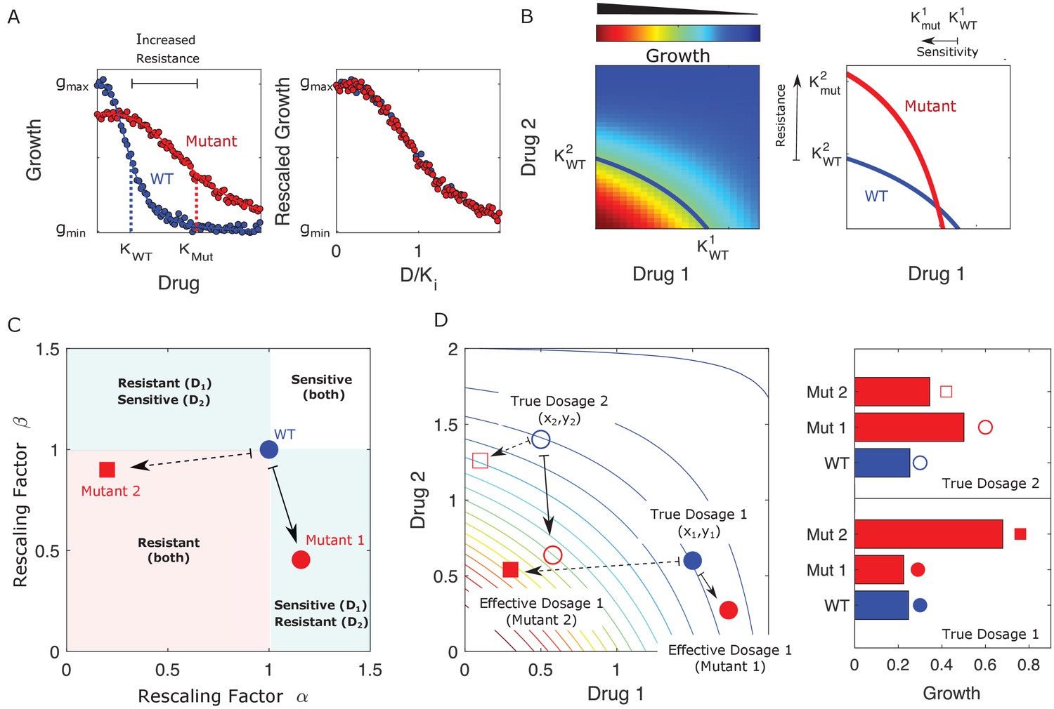
Drug resistance as a rescaling of effective drug concentration.
The fundamental assumption of our model is that drug-resistant mutants exhibit phenotypes identical to those of the ancestral (‘wild type’) cells but at rescaled effective drug concentration. (A) Left panel: schematic dose-response curves for an ancestral strain (blue) and a resistant mutant (red). Half-maximal inhibitory concentrations (,), which provide a measure of resistance, correspond to the drug concentrations where inhibition is half maximal. Fitness cost of resistance is represented as a decrease in drug-free growth. Right panel: dose-response curves for both cell types collapse onto a single functional form, similar to those in Chait et al., 2007; Michel et al., 2008; Wood and Cluzel, 2012; Wood et al., 2014. (B) Left panel: in the presence of two drugs, growth is represented by a surface; the thick blue curve represents the isogrowth contour at half-maximal inhibition; it intersects the axes at the half-maximal inhibitory concentrations for each individual drug. Right panel: isogrowth contours for ancestral (WT) and mutant cells. In this example, the mutant exhibits increases resistance to drug 2 and an increased sensitivity to drug 1, each of which corresponds to a rescaling of drug concentration for that drug. These rescalings are quantified with scaling constants and , where the superscripts indicate the drug (1 or 2). (C) Scaling factors for two different mutants (red square and red circle) are shown. The ancestral cells correspond to scaling constants . Mutant 1 exhibits increased sensitivity to drug 1 () and increased resistance to drug 2 (). Mutant 2 exhibits increased resistance to both drugs (), with higher resistance to drug 1. (D) Scaling parameters describe the relative change in effective drug concentration experienced by each mutant. While scaling parameters for a given mutant are fixed, the effects of those mutations on growth depend on the external environment (i.e., the drug dosage applied). This schematic shows the effective drug concentrations experienced by WT cells (blue circles) and the two different mutants (red circles and red squares) from panel (C) under two different external conditions (open and closed shapes). True dosage 1 (2) corresponds to higher external concentrations of drug 1 (2). The concentrations are superimposed on a contour plot of the two drug surface (similar to panel B). Right panel: resulting growth of mutants and WT strains at dosage 1 (bottom) and dosage 2 (top). Because the dosages are chosen along a contour of constant growth, the WT exhibits the same growth at both dosages. However, the growth of the mutants depends on the dose, with mutant 1 growing faster (slower) than mutant 2 under dosage 2 (dosage 1). A key simplifying feature of these evolutionary dynamics is that the selective regime (drug concentration) and phenotype (effective drug concentration) have same units.
Figure 1—video 1
Detailed selection dynamics associated to Figure 2.
Here we visualize the selection going on in a hypothetical bacterial population under the two-drug dosage-selective regime ( and growth landscape shown in Figure 2, where the collateral effects, represented in the available mutants (), are estimated from data (Figure 3—figure supplement 1C). The size of the circles in rescaling factor trait space corresponds to the relative frequency of each subpopulation, calculated at each timepoint.
Figure 2

Using the rescaling framework for predicting resistance evolution to two drugs in a population of bacterial cells.
(A) Growth landscape (per capita growth rate relative to untreated cells) as a function of drug concentration for two drugs (drug 1, tigecycline; drug 2, ciprofloxacin; concentrations measured in μg/mL) based on measurements in Dean et al., 2020. We consider evolution of resistance in a population exposed to a fixed external drug concentration ( (white asterisk). (B) Growth landscape from (A) with axes rescaled to reflect scaling parameters (). The point in drug concentration space now corresponds to the point in scaling parameter space; intuitively, a strain characterized by scaling parameters of unity experiences an effective drug concentration equal to the true external concentration. We consider a population that is primarily ancestral cells (fraction 0.99), with the remaining fraction uniformly distributed between an empirically measured collection of mutants (each corresponding to a single pair of scaling parameters, white circles). At time 0, the population is primarily ancestral cells and is therefore centered very near (gray circle). Over time, the mean value of each scaling parameter decreases as the population becomes increasingly resistant to each drug (black curve). (C) The two-dimensional mean scaling parameter trajectory from (B) plotted as two time series, one for α (red) and one for β (blue). For the detailed selection dynamics, see Figure 1—video 1. (D) The mean fitness of the population during evolution is expected to increase and can be computed from the selection dynamics by numerically integrating the model at each time step.
Figure 3 with 5 supplements
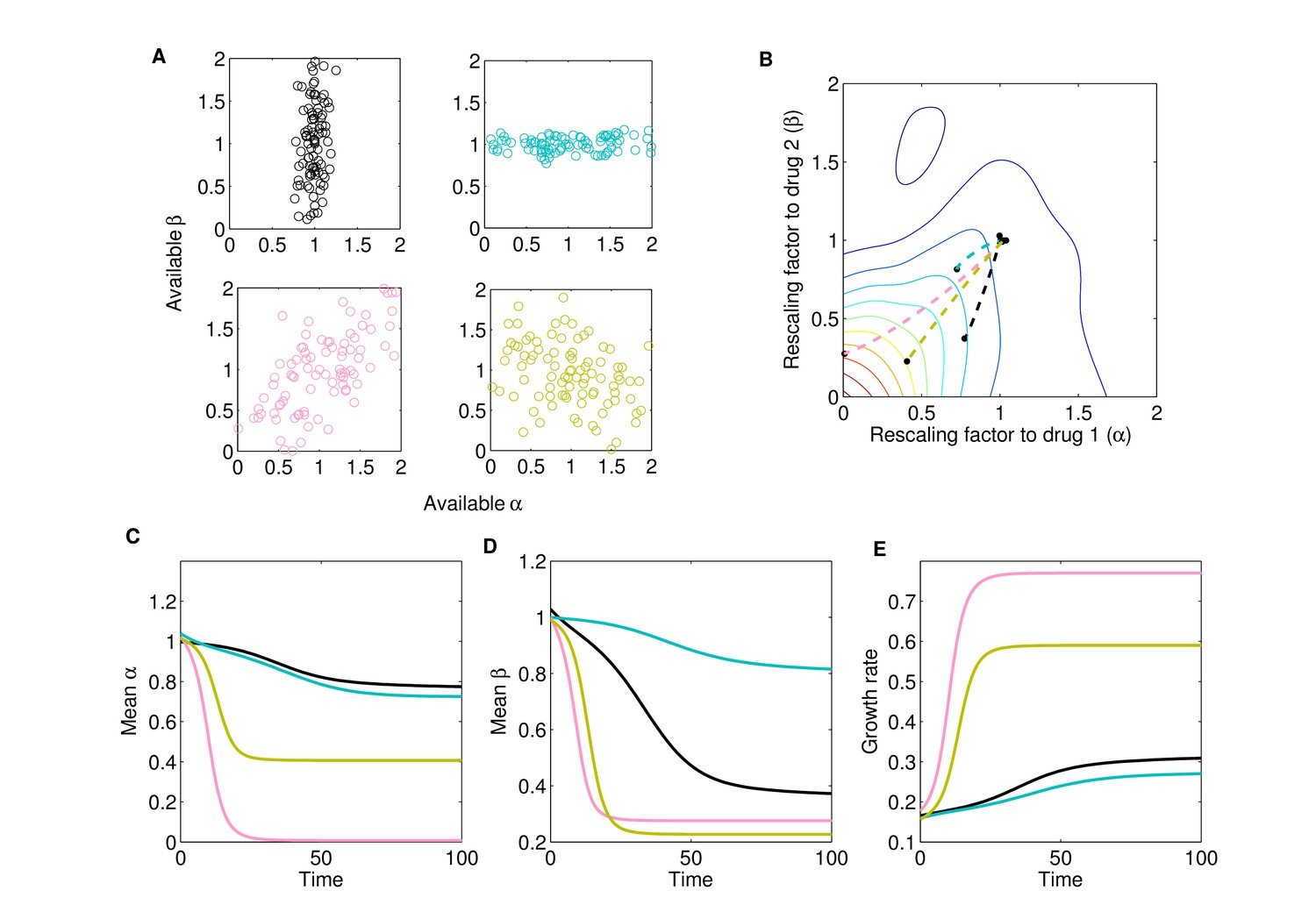
Different collateral profiles drive different evolutionary dynamics under the same treatment.
We simulated random collateral profiles for susceptibilities to two drugs and use them to predict phenotypic trajectories of a bacterial population. For the two-drug landscape, we chose one of the experimentally measured surfaces from Dean et al., 2020; Figure 3—figure supplement 1C, corresponding to the drug combination TGC-CIP (drug 1-drug 2). (A) Four special profiles include predominant variation in β (black), predominant variation in α (cyan), positive correlation between αs and βs (pink), and negative correlation between the susceptibilities to the two drugs (green). These were generated from a bivariate normal distribution with mean and covariance matrices , , , . (B) The trajectories in mean space following treatment (), with and , corresponding to different collateral profiles. (C) The dynamics of mean susceptibility to drug 1 for the four cases. (D) The dynamics of mean susceptibility to drug 2 for the four cases. (E) The dynamics of mean growth rate for the four cases. For underlying heterogeneity, we drew 100 random and as shown in (A) and initialized dynamics at ancestor frequency 0.99 and the remaining 1% evenly distributed among available mutants. It is clear that each collateral structure in terms of the available leads to different final evolutionary dynamics under the same two-drug treatment. In this particular case, the fastest increase in resistance to two drugs and increase in growth rate occurs for the collateral resistance (positive correlation) case. The time course of the detailed selective dynamics in these four cases is depicted in Figure 3—videos 1–4.
Figure 3—figure supplement 1

Response surfaces and scaling parameters for three drug pairs.
Growth rate surfaces (left) and scaling parameters α and β for three drug combinations: ampicillin (AMP)-streptomycin (STR) (A); ceftriaxone (CRO)-ciprofloxacin (CIP) (B); and ciprofloxacin (CIP)-tigecycline (TGC) (C). Large color-coded circles on the left panels indicate external concentrations at which selection took place. Circles on the right panels indicate all observed mutants () that emerged, pooled across conditions. Data from Dean et al., 2020. Growth rate is measured in normalized units where growth of the drug-free ancestral cells (approximately 1 hr−1) is set to 1.
Figure 3—video 1
Evolutionary dynamics for collateral effects in Figure 3A.
Trajectory of mean traits in rescaling factor space () for case A in Figure 3 where the randomly generated available standing variation is higher in β (resistance to drug 2) and much lower in α (resistance to drug 1). The selective regime in drug dosage is . The size of the circles at t=0,... represents the relative frequencies of different mutant subpopulations available at the beginning and changing over time.
Figure 3—video 2
Evolutionary dynamics for collateral effects in Figure 3B.
Trajectory of mean traits in rescaling factor space () for case A in Figure 3 where the randomly generated available standing variation is lower in β and higher in α. The selective regime in drug dosage is . The dynamic size of the circles represents the relative frequencies of different mutant subpopulations available at the beginning and changing over time.
Figure 3—video 3
Evolutionary dynamics for collateral effects in Figure 3C.
Trajectory of mean traits in rescaling factor space () for case A in Figure 3 where the randomly generated available standing variation in β correlates positively with that in α (collateral resistance between the two drugs TGC-CIP). The selective regime in drug dosage is . The dynamic size of the circles represents the changing relative frequencies of different mutant subpopulations.
Figure 3—video 4
Evolutionary dynamics for collateral effects in Figure 3B.
Trajectory of mean traits in rescaling factor space () for case A in Figure 3 where the randomly generated available standing variation in β correlates negatively with that in α (collateral sensitivity between TGC and CIP). The selective regime in drug dosage is . The size of the circles represents the relative frequencies of different mutant subpopulations available at the beginning.
Figure 4 with 1 supplement
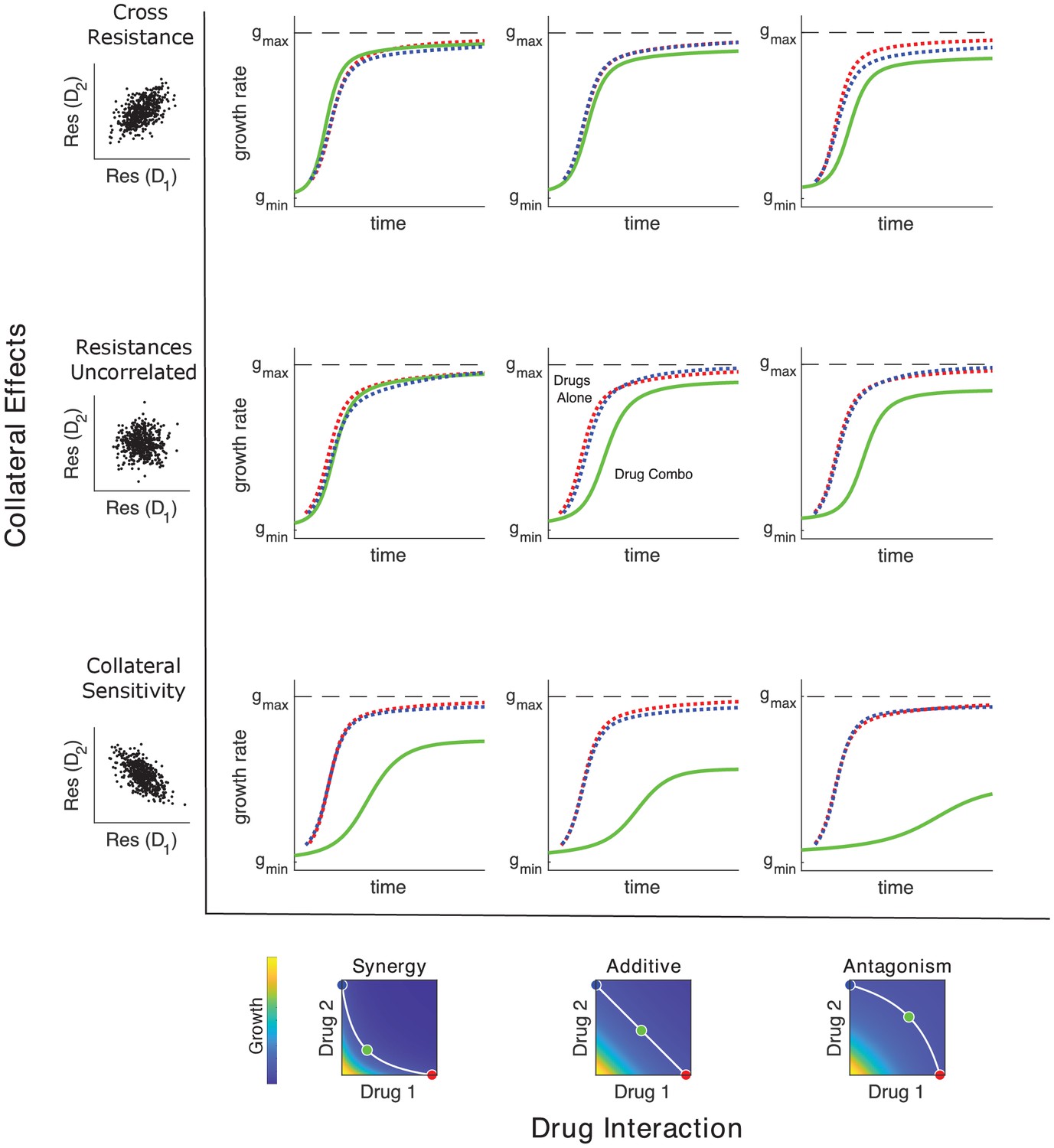
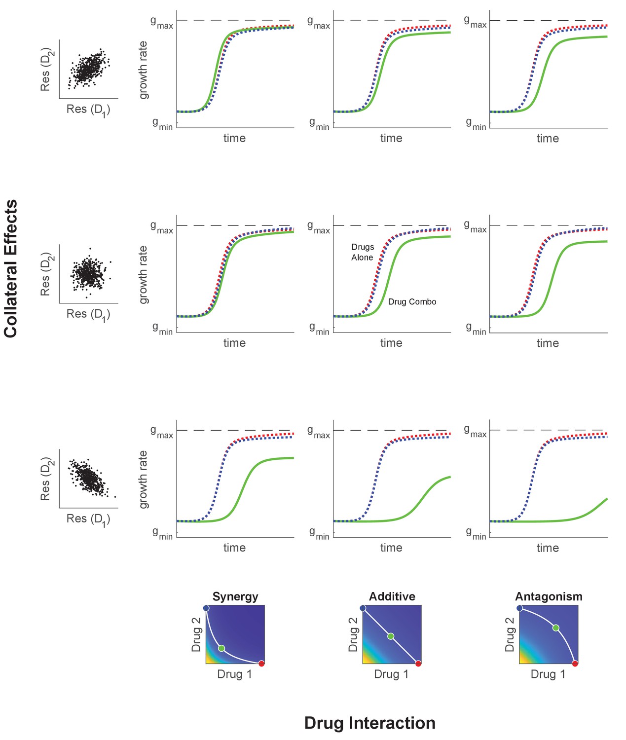
Adaptation depends on drug interactions and collateral effects of resistance.
Drug interactions (columns) and collateral effects (rows) modulate the rate of growth adaptation (main nine panels). Evolution takes place at one of three dosage combinations (blue, drug 2 only; cyan, drug combination; red, drug 1 only) along a contour of constant growth in the ancestral growth response surface (bottom panels). Drug interactions are characterized as synergistic (left), additive (center), or antagonistic (right) based on the curvature of the isogrowth contours. Collateral effects describe the relationship between the resistance to drug 1 and the resistance to drug 2 in an ensemble of potential mutants. These resistance levels can be positively correlated (top row, leading to collateral resistance), uncorrelated (center row), or negatively correlated (third row, leading to collateral sensitivity). Growth adaptation (main nine panels) is characterized by growth rate over time, with dashed lines representing evolution in single drugs and solid lines indicating evolution in the drug combination. In this example, response surfaces are generated with a classical pharmacodynamic model (symmetric in the two drugs) that extends Loewe additivity by including a single-drug interaction index that can be tuned to create surfaces with different combination indices (Greco et al., 1995). The initial population consists of primarily ancestral cells along with a subpopulation 10−2 mutants uniformly distributed among the different phenotypes. Scaling parameters are sampled from a bivariate normal distribution with equal variances () and correlation ranging from 0.6 (top row) to −0.6 (bottom row). See also Figure 4—figure supplement 1 for gradient approximation to selection dynamics.
Figure 4—figure supplement 1
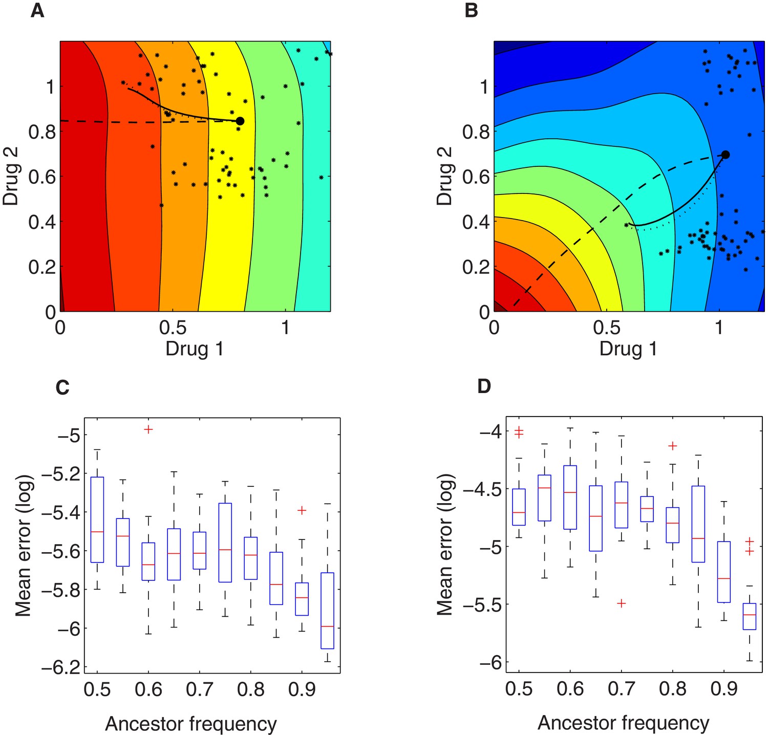
Illustration of the local growth gradient approximation to the Price equation.
(A, B) Comparison between numerical solutions to the full Price equation (dotted line), the local growth gradient approximation (solid line), and the trajectory of pure (unweighted) gradient descent (dashed line) for mean resistance evolution to two drugs (). The dotted and solid lines are almost indistinguishable. In (A) and (B), we assume two growth landscapes respectively (drug combination 1 vs. drug combination 3, see Figure 3—figure supplement 1A, C), external concentrations , and initial trait distributions following the empirically derived (. The large black dot represents the initial value () under initial ancestor frequency of 90% and the remaining 10% spread uniformly among available mutants (denoted via the small black asterisks in the 2-D trait space). (C, D) Root mean square error between mean trait evolution calculated with the full iteration of the Price equation and the gradient approximation (for the two cases in A and B, respectively), varying ancestor initial frequency. Here for each (the initial frequency of the ancestor subpopulation with scaling parameters ), we simulated 20 stochastic realizations of the evolutionary process under drug dosage , starting from different random frequencies for the remaining proportion of the population composed of available mutants.
Figure 5 with 5 supplements
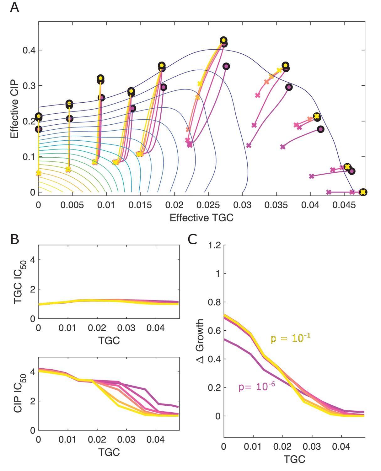
Drug rescaling describes adaptation dynamics of growth and drug resistance in Enterococcus faecalis under different selective regimes.
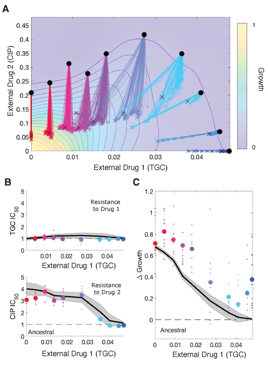
(A) Experimentally measured growth response surface for tigecycline (TGC) and ciprofloxacin (CIP). Circles represent 11 different adaptation conditions, each corresponding to a specific dosage combination . Solid lines show 100 simulated adaptation trajectories (i.e., changes in effective drug concentration over time: mean D1eff D2eff, for a total time ) predicted from the full rescaling model. Black xs indicate the mean (across all trajectories) value of the effective drug concentration at the end of the simulation. In each case, the set of available mutants – and hence, the set of possible scaling parameters αi and βi – is probabilistically determined by uniformly sampling approximately 10 scaling parameter pairs from the ensemble experimentally measured across parallel evolution experiments involving this drug pair (see Materials and methods). (B) Half-maximal inhibitory concentration (IC50, normalized by that of the ancestral strain) for populations adapted for a fixed time period hr in each of the 11 conditions in the top panel. The solid curve is the mean trajectory from the rescaling model (normalized IC50 corresponds to the reciprocal of the corresponding scaling constant) for 100 simulated samples of the scaling parameter pairs; shaded region is ±1 standard deviation over all trajectories. Small circles are experimental observations from individual populations; larger markers are average experimental results over all populations adapted to a given condition. Note that drug 1 (TGC) concentration (x-axis) here is just a proxy for the different conditions as you move left to right along the contour in panel (A). (C) Change in population growth rate (, where is per capita growth of ancestral strain and for the mutant; all growth rates are normalized to ancestral growth in the absence of drugs) for populations adapted in each condition. Solid curve is the mean trajectory across samplings, with shaded region ±1 standard deviation. Small circles are results from individual populations; larger markers are averages over all populations adapted to a given condition. Experimental data from Dean et al., 2020. See also Figure 5—figure supplements 1–5.
Figure 5—figure supplement 1
Model captures qualitative features of experimental evolution in combinations of ampicillin (AMP) and streptomycin (STR).
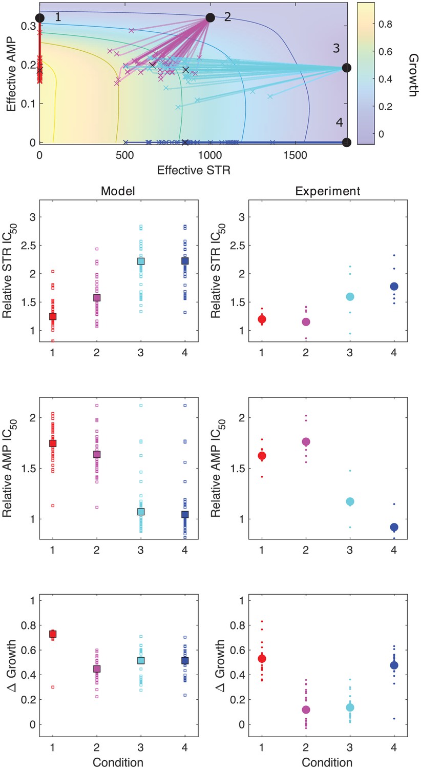
Top panel: experimentally measured growth response surface for AMP and STR. Circles represent four different adaptation conditions, each corresponding to a specific dosage combination . Solid lines show adaptation trajectories (i.e., changes in effective drug concentration over time) predicted from the Price equation over an interval t = 48 hr. In each case, the set of available mutants – and hence, the set of possible scaling parameters α and β – is determined by sampling from experimentally measured changes in resistance (half-maximal inhibitory concentration IC50) for each drug in the full ensemble of mutants arising from adaptation to these drugs (see Figure 3—figure supplement 1). Bottom panels: comparing results from the model (left column) and experiment (right panel). Quantities include relative change in IC50 for each drug (top two rows) as well as overall change in population growth (bottom row); in each case, results are shown for each of the four conditions in the top panel. For the experiments, small markers are results from individual populations; larger markers are averages over all populations adapted to a given condition. For the model, small markers are results from each subsampling of the experimental scaling parameters (approximately 10 per run); larger markers are averages over all subsamples. Experimental data from Dean et al., 2020.
Figure 5—figure supplement 2

Model captures qualitative features of experimental evolution in combinations of ceftriaxone (CRO) and ciprofloxacin (CIP).
Top panel: experimentally measured growth response surface for CRO and CIP. Circles represent four different adaptation conditions, each corresponding to a specific dosage combination . Solid lines show adaptation trajectories (i.e., changes in effective drug concentration over time) predicted from the Price equation over an interval t = 48 hr. In each case, the set of available mutants – and hence, the set of possible scaling parameters α and β – is determined by sampling from experimentally measured changes in resistance (half-maximal inhibitory concentration IC50) for each drug in the full ensemble of mutants arising from adaptation to these drugs (see Figure 3—figure supplement 1). Bottom panels: comparing results from the model (left column) and experiment (right panel). Quantities include relative change in IC50 for each drug (top two rows) as well as overall change in population growth (bottom row); in each case, results are shown for each of the four conditions in the top panel. For the experiments, small markers are results from individual populations; larger markers are averages over all populations adapted to a given condition. For the model, small markers are results from each subsampling of the experimental scaling parameters; larger markers are averages over all subsamples. Experimental data from Dean et al., 2020.
Figure 5—figure supplement 3
Resampling ensemble of scaling parameters does not dramatically impact dynamics.
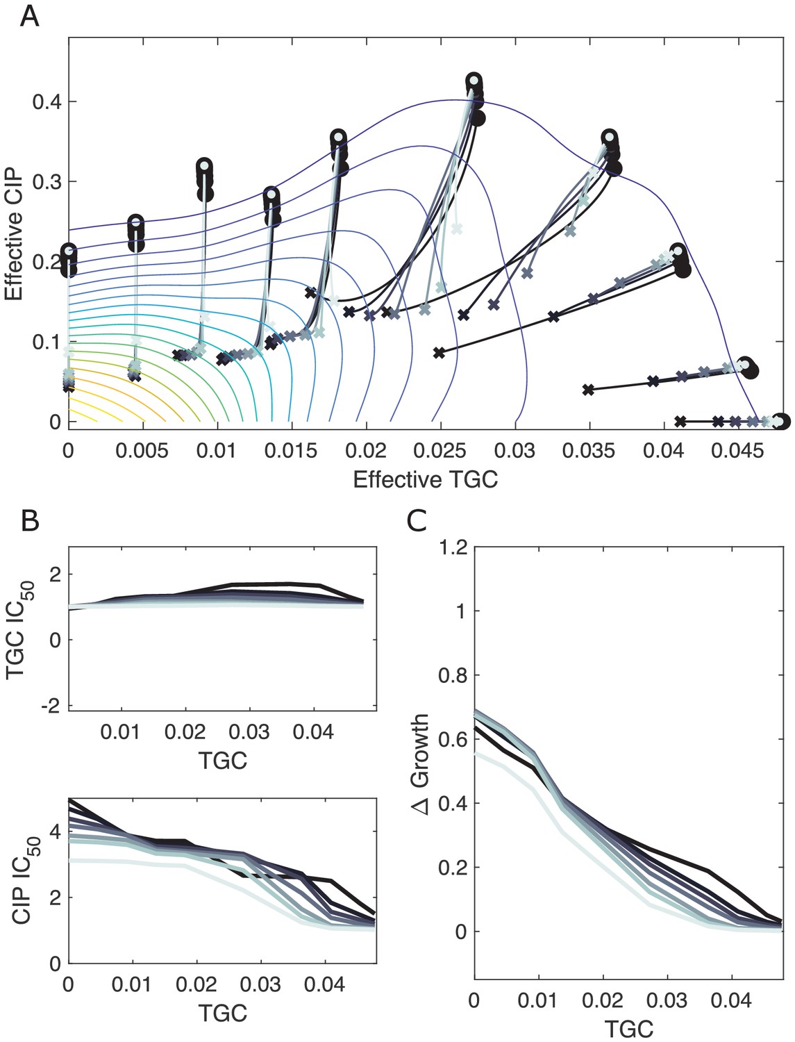
(A) Experimentally measured growth response surface for tigecycline (TGC) and ciprofloxacin (CIP) from Dean et al., 2020. Circles represent 11 different adaptation conditions, each corresponding to a specific dosage combination . Solid lines show the mean adaptation trajectories (i.e., changes in effective drug concentration over time) predicted from the Price equation. In each case, the set of available mutants – and hence, the set of possible scaling parameters α and β – is determined by sub-sampling pairs from experimentally measured scaling parameters (from a total of 72 pairs). Different curves are averages over 100 realizations (samples) of (darkest), , , , , , and (lightest) pairs. In each realization, the ancestor frequency () was fixed at 99% and the remaining 1% was randomly spread among the available mutants. (B) Predicted change in IC50 for populations adapted in each of the 11 conditions in (A). (C) Predicted change in population growth rate for populations adapted in each condition in (A).
Figure 5—figure supplement 4
Different estimates of total time lead to similar qualitative dynamics.
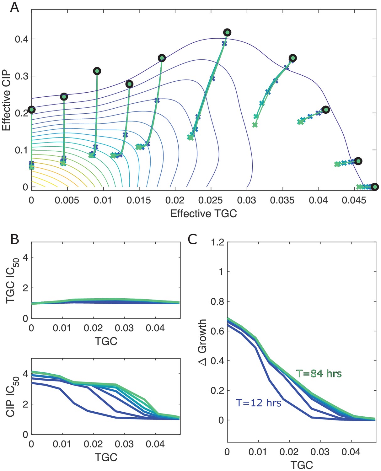
(A) Experimentally measured growth response surface for tigecycline (TGC) and ciprofloxacin (CIP) from Dean et al., 2020. Circles represent 11 different adaptation conditions, each corresponding to a specific dosage combination . Solid lines show the mean adaptation trajectories (i.e., changes in effective drug concentration over time) predicted from the Price equation. In each case, the set of available mutants – and hence, the set of possible scaling parameters α and β – is determined by sampling pairs (αi,βi) from experimentally measured scaling parameters (from a total of 72 pairs). Different curves are averages over 100 realizations (samples) for total simulation times ranging from to hr. In each realization, the ancestor frequency () was fixed at 99% and the remaining 1% was randomly spread among the available mutants. (B) Predicted change in IC50 for simulated populations adapted in each of the 11 conditions in (A). (C) Predicted change in population growth rate for populations adapted in each condition in (A). In panels (B) and (C), the horizontal axis (TGC) is the external concentration of tigecycline (μg/mL) used in each selecting condition in (A).
Figure 5—figure supplement 5
Different estimates of initial resistant fraction lead to similar qualitative dynamics.
(A) Experimentally measured growth response surface for tigecycline (TGC) and ciprofloxacin (CIP) from Dean et al., 2020. Circles represent 11 different adaptation conditions, each corresponding to a specific 2-drug dosage combination . Solid lines show the mean adaptation trajectories (i.e., changes in effective drug concentration over time) predicted from the Price equation. In each case, the set of available mutants – and hence, the set of possible scaling parameters α and β – is determined by sampling pairs from experimentally measured scaling parameters (from a total of 72 pairs). Different curves are averages over 100 realizations (samples) for initial mutant fractions ranging from to hr. In each realization, the dynamics were simulated for a total time of hr. (B) Predicted change in IC50 for simulated populations adapted in each of the 11 conditions in (A). (C) Predicted change in population growth rate for populations adapted in each condition in (A). In panels (B) and (C), the horizontal axis (TGC) is the external concentration of tigecycline (μg/mL) used in each selecting condition in (A).
Figure 6 with 4 supplements
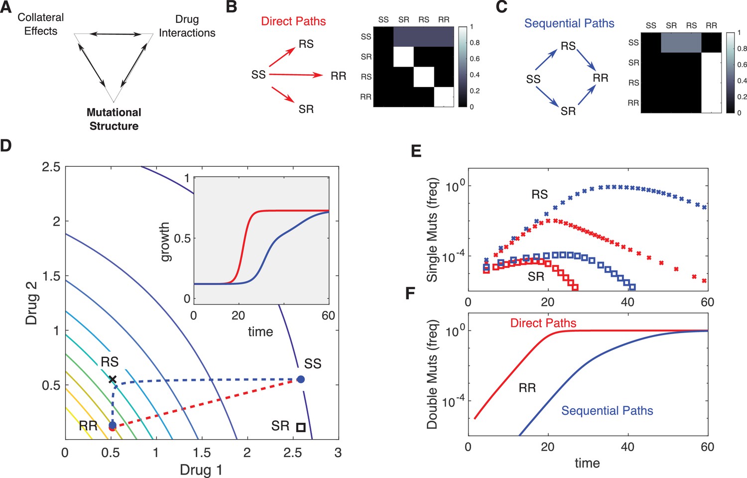
Incorporating mutational structure modulates evolutionary dynamics.
(A) Evolutionary dynamics reflect a combination of collateral effects, drug interactions, and mutational structure. (B) Phenotypes are defined by relative resistance (R) or sensitivity (S) to each of two drugs, leading to four possible phenotypes: SS , RS , SR , or RR . Mutations can occur via direct paths (B), where each mutant phenotype is accessible directly from the fully sensitive ancestor, or via sequential paths (C), where the doubly resistant mutant (RR) is only accessible from single mutants (RS or SR). Entries of the mutation matrix (heatmaps) reflect the probability of mutating from state (rows) to state (columns) given that a mutation occurs in state . (D) Main panel: contour plot of growth surface in ancestral (SS) cells. For a specific choice of drug dosages, SS cells experience the true dosage combination (; blue circle, SS) while single mutants (black x, RS; and black square, SR) and double-resistant mutants (RR) experience decreased effect concentration of one or more drugs. Dashed lines show mean trajectories () for direct (red) and sequential (blue) mutational structures. Inset: mean growth rate for direct (red) and sequential (blue) mutational structures. (E, F) Population frequencies for single mutants (panel D; xs are RS, squares are SR) and double mutants (panel E) under direct (red) or sequential (blue) mutational structures. See also Figure 6—figure supplements 1–4.
Figure 6—figure supplement 1
Adaptation in the presence of mutation depends on drug interaction and collateral effects of resistance.
Similar to Figure 4, but with initial population composed entirely of ancestral cells and an assumed mutation rate . The mutation matrix allows mutations to occur with equal probability from the WT to any of the available mutants. Drug interaction (columns) and collateral effects (rows) modulate the rate of growth adaptation (main nine panels). Evolution takes place at one of three dosage combinations (blue, drug 2 only; cyan, drug combination; red, drug 1 only) along a contour of constant growth in the ancestral growth response surface (bottom panels). Drug interactions are characterized as synergistic (left), additive (center), or antagonistic (right) based on the curvature of the isogrowth contours. Collateral effects describe the relationship between the resistance to drug 1 and the resistance to drug 2 in an ensemble of potential mutants. These resistance levels can be correlated (top row, leading to collateral resistance), uncorrelated (center row), or anticorrelated (third row, leading to collateral sensitivity). Growth adaptation (main nine panels) is characterized by growth rate over time, with dashed lines representing evolution in single drugs and solid lines indicating evolution in the drug combination. In this example, response surfaces are generated with a classical pharmacodynamic model that extends Loewe additivity by including a single-drug interaction index that can be tuned to create surfaces with different combination indices (Greco et al., 1995).
Figure 6—figure supplement 2
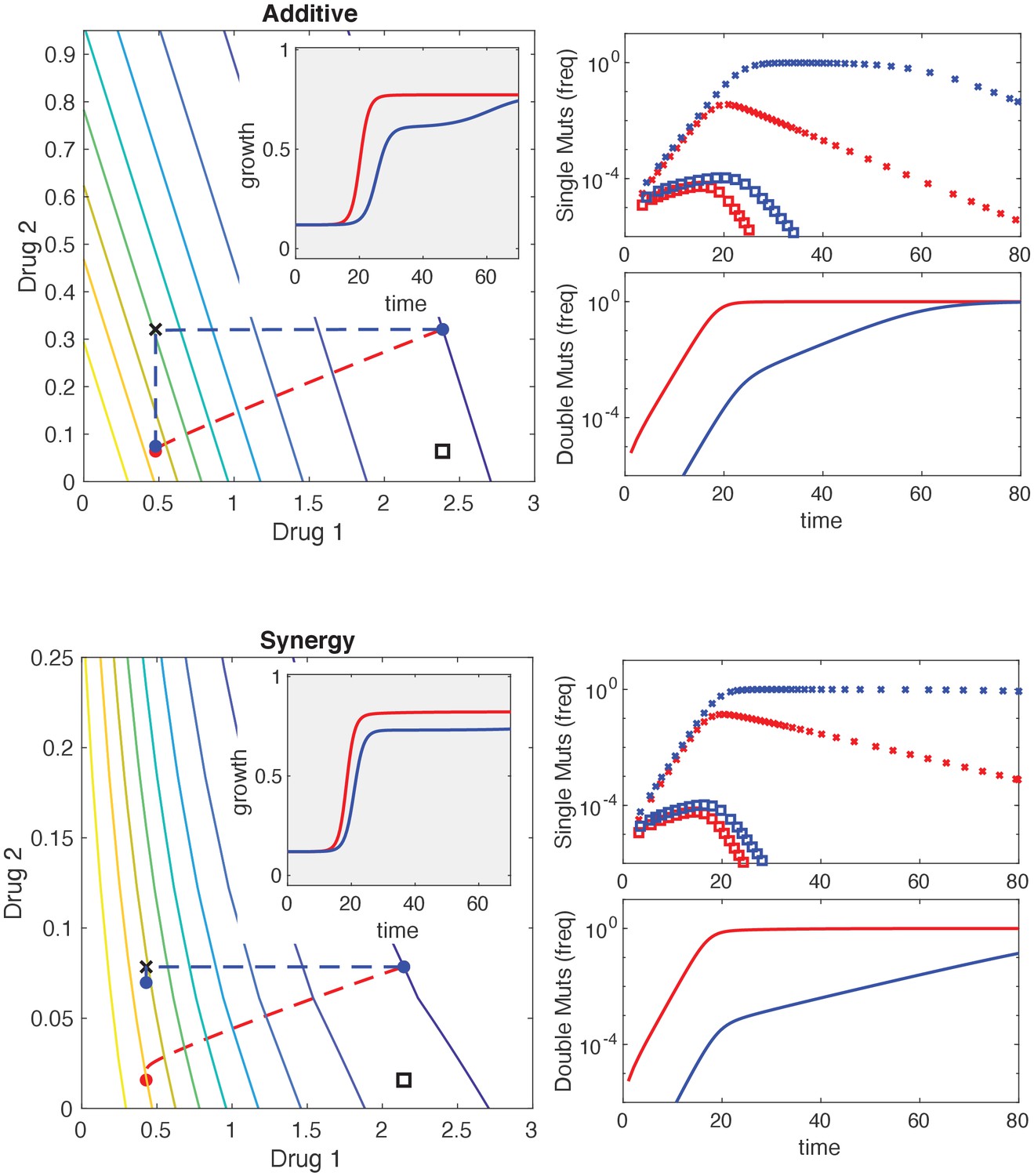
Mutational structure modulates evolutionary dynamics for additive and synergistic drug combinations.
Top and bottom panels are identical to Figure 6 but with additive (top) and synergistic (bottom) drug interactions. Phenotypes are defined by resistance (R) or sensitivity (S) to each of two drugs, leading to four possible phenotypes: SS , RS , SR , or RR . Mutations can occur via direct paths, where each mutant phenotype is accessible directly from the fully sensitive ancestor, or via sequential paths, where the doubly resistant mutant (RR) is only accessible from single mutants (RS or SR). Main left panel: contour plot of growth surface in ancestral (SS) cells. For a specific choice of drug dosages, SS cells experience the true dosage combination (; blue circle, SS) while single mutants (black x, RS; and black square, SR) and double-resistant mutants (RR) experience decreased effect concentration of one or more drugs. Dashed lines show mean trajectories () for direct (red) and sequential (blue) mutational structures. Inset: mean growth rate for direct (red) and sequential (blue) mutational structures. Right panels: population frequencies for single mutants (upper panel; xs are RS, squares are SR) and double mutants (lower panel) under direct (red) or sequential (blue) mutational structures.
Figure 6—figure supplement 3
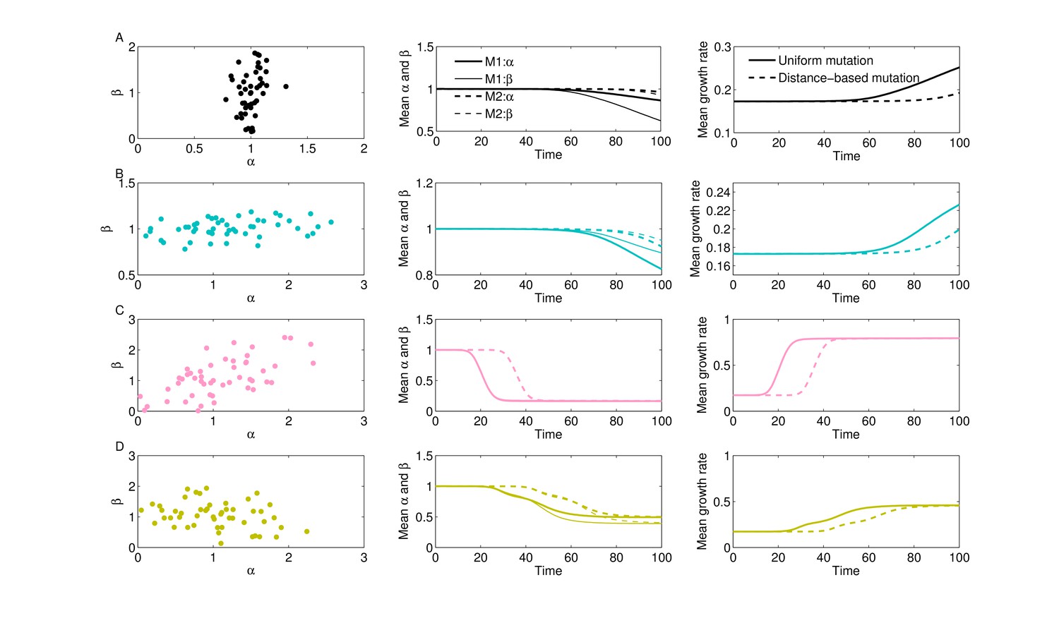
Uniform vs. distance-based mutation and evolutionary dynamics for 4 collateral structures.
We generated the same four collateral structures (A–D) for correlations between and as in Figure 3 and used the same growth surface for drug interactions. Instead of setting initial frequencies as non-zero, here we started simulations with 100% WT, at trait (1,1) and allowed other subpopulations to arise via mutation. We used a mutation rate . Mutations can occur with uniform rates (M1) or via distance-based scalings (M2), where mutant phenotype is accessible from all mutants but with higher probability if is closer in the space of scaling parameters (, with the Euclidean distance between pairs of scaling parameters in () space). We summarize 10 stochastic realizations for each collateral structure. Solid lines show mean system trajectories for uniform mutation, whereas dashed lines show mean trajectories of mean traits () for distance-based mutation.
Figure 6—figure supplement 4
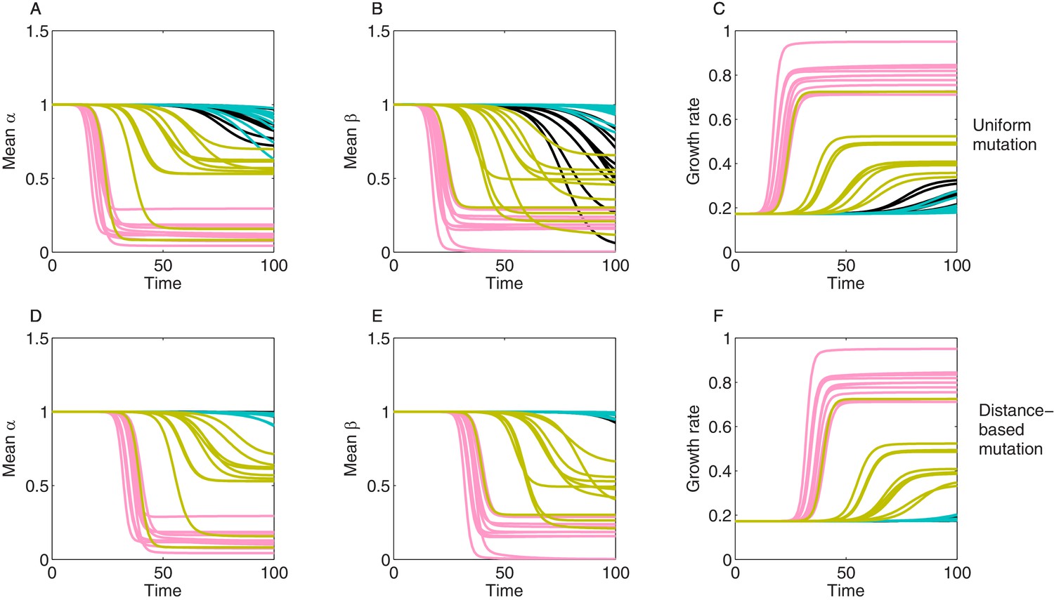
Stochastic realizations of collateral structures and evolutionary dynamics under two mutation models.
We show here 10 stochastic realizations for each generated collateral structure (like in Figure 6—figure supplement 3, Figure 3) for correlations between and and used the same growth surface for drug interactions. We started simulations with 100% WT, at trait (1,1) and allowed 100 other subpopulations to arise via mutation. We used a mutation rate . Mutations can occur with uniform rates (M1) (A–C) or via distance-based scalings (M2) (D–F), where mutant phenotype is accessible from all mutants but with higher probability if is closer , and the distance metric being, for example, the Euclidean distance in () space. (A, D) show mean resistance evolution to drug 1. (B, E) show mean resistance evolution to drug 2. (C, F) show mean growth rate dynamics. Different colors indicate different collateral structures, and different lines depict different sampled mutants () from the same distribution.
Figure 7 with 2 supplements
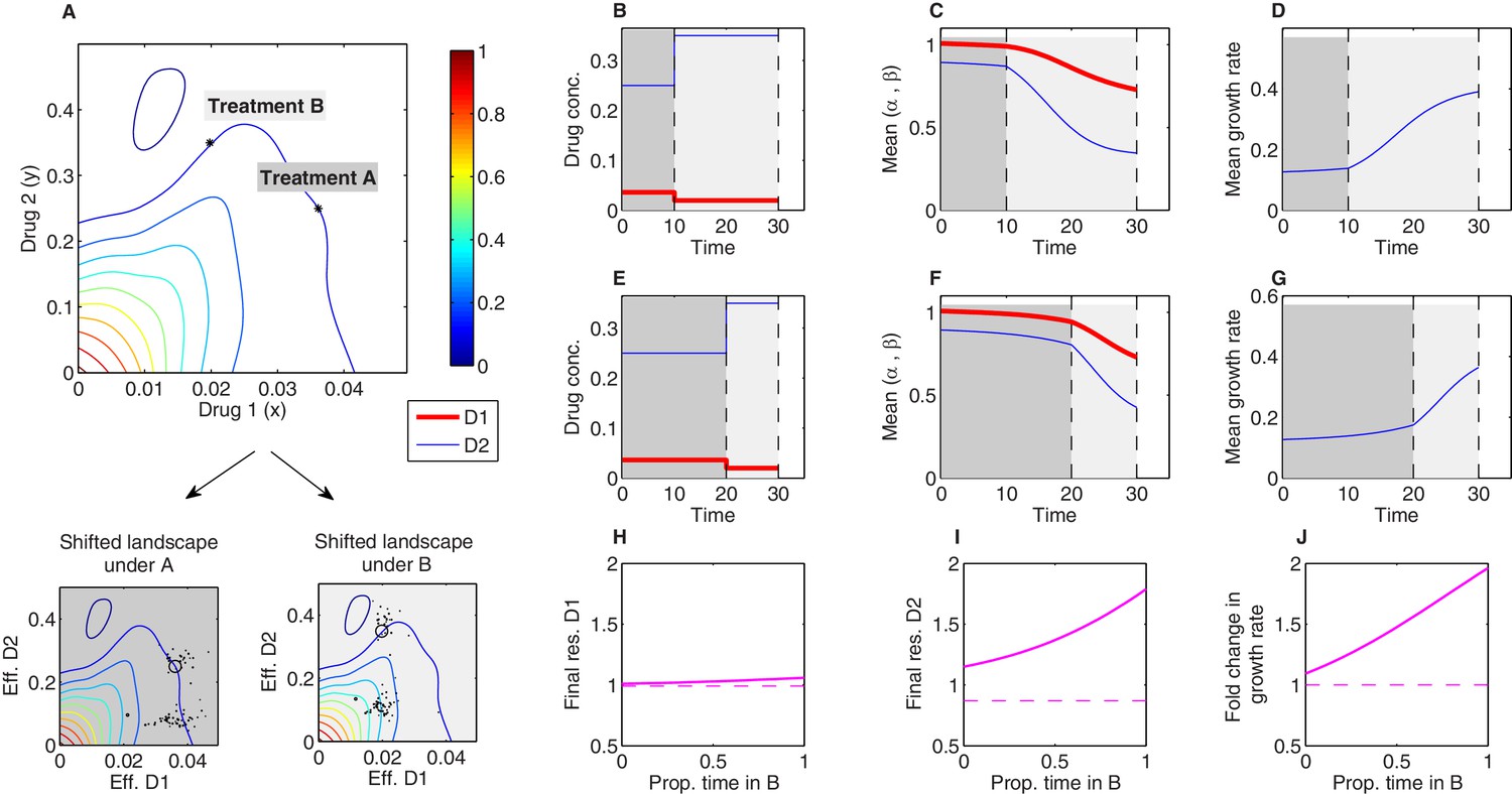
Sequential multidrug treatments lead to different evolutionary outcomes under different schedules.
The model framework can be used to predict phenotypic evolution and growth dynamics in a bacterial population under consecutive treatments involving different dosage combinations of the same two drugs. (A) Treatments A and B (asterisks) are chosen to lie along a contour of constant growth in the space of drug concentrations. Two-drug growth surface (top panel) and the collection of scaling parameter pairs are based on data from Dean et al., 2020 for tigecycline (drug 1) and ciprofloxacin (drug 2). The same set of scaling parameters leads to different effective drug concentrations when exposed to treatment A (bottom-left panel; each mutant is represented by a single point representing the effective concentration of each drug) and treatment B (bottom-right panel). (B-G) Time series of drug concentrations (B, E), mean scaling parameters (C, F), and mean growth rate (D, G) for sequential treatments (treatment A followed by treatment B). Panels (B–D) correspond to a short epoch (10 time units) of A followed by a longer (20 time units) epoch of B. Panels (E–G) correspond to a long epoch of A followed by a shorter epoch of B. (H–J) Changes in resistance to drug 1 () (H), resistance to drug 2 () (I), and growth rate (J) for treatments of a fixed length ( time units) but varying the fraction of time spent in each treatment. Each treatment consisting of one epoch of A (for time ) followed by one epoch of B (for time ). See also Figure 7—figure supplement 1 (for detailed temporal trajectories) and Figure 7—figure supplement 2 (for longer total therapies with saturating dynamics). In all panels, we assumed mutants were characterized by scaling parameter pairs ( and ) measured experimentally (Figure 3—figure supplement 1). Initial populations consisted of primarily ancestral cells (fraction 0.99), while the remaining population (fraction 0.01) was uniformly distributed among all available mutants.
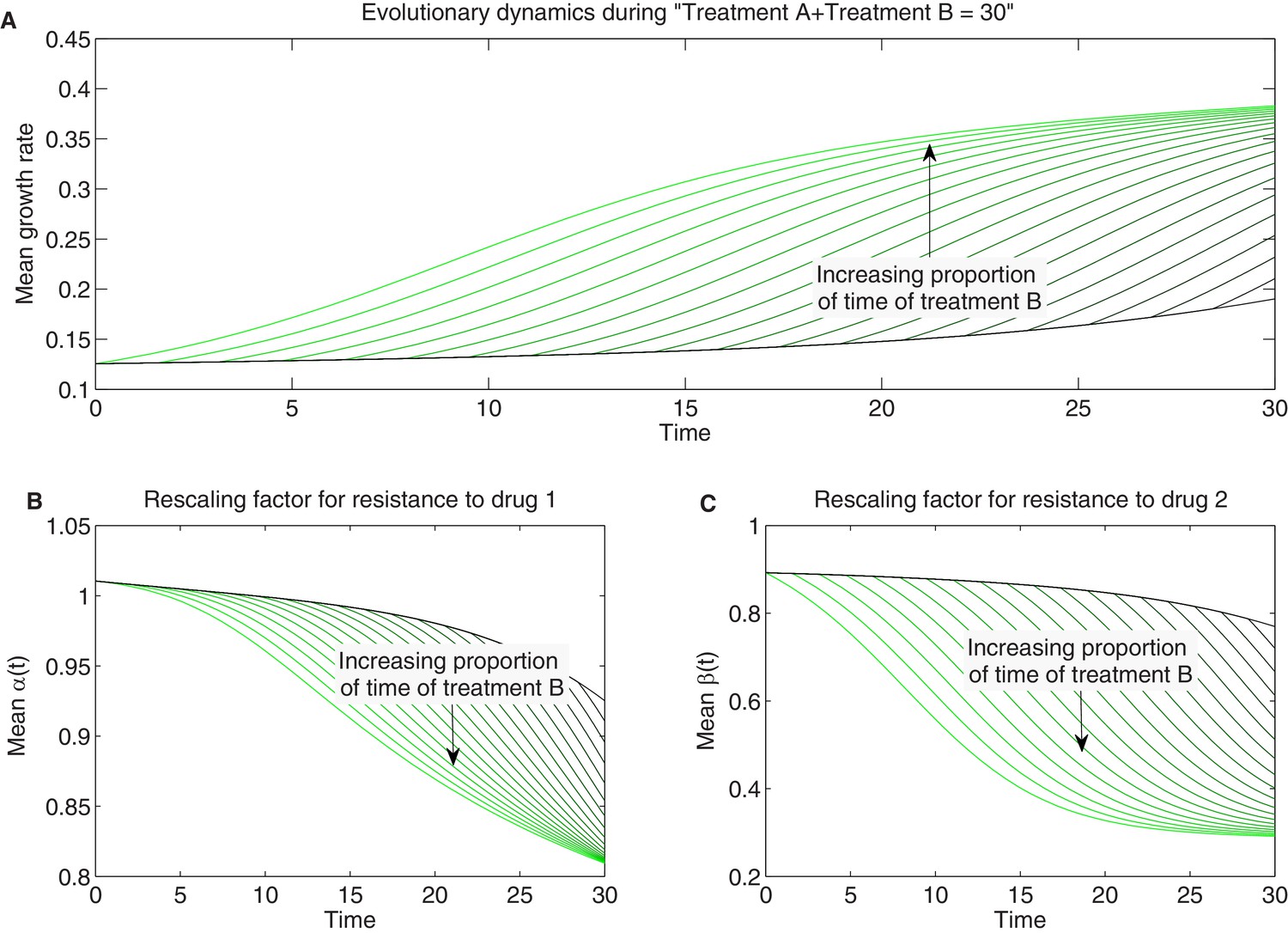
Figure 7—figure supplement 1
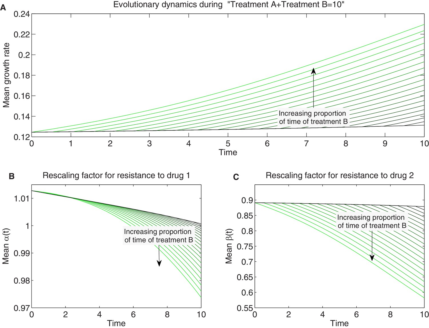
Detailed temporal trajectories of population mean traits and growth rate under sequential two-drug therapies.
We combined sequentially treatments A and B in Figure 7 in different proportions amounting to a total hours of therapy. Treatment A combines drugs 1 and 2 in the concentrations and B in the concentrations . Panels show time series of mean growth rate (A) and mean scaling parameters (B-C).
Figure 7—figure supplement 2
Detailed temporal trajectories of population mean traits and growth rate under sequential two-drug therapies for longer total duration.
We combined sequentially two-drug treatments: treatment A and B in Figure 7 in different proportions amounting to a total duration of hr of therapy. As time of therapy is increased (compare to Figure 7—figure supplement 1) and selection proceeds further to select high-fitness mutants, the space of available mutants is exhausted and evolutionary trajectories saturate. Panels show time series of mean growth rate (A) and mean scaling parameters (B-C).
Tables
Table 1
Different biological properties correspond to different features of the model.
| Biological property | Model property |
|---|---|
| Scaling parameters (ancestral) | |
| Resistance to drug 1* | Inverse scaling parameter |
| Resistance to drug 2* | Inverse scaling parameter |
| Synergistic interaction | Locally convex isoboles in 2-drug growth surface |
| Antagonistic interaction | Locally concave isoboles in 2-drug growth surface |
| Cross-resistance | Positively correlated scaling parameters () |
| Collateral sensitivity | Negatively correlated scaling parameters () |
| External concentration () | Effective drug concentration () |
| Fitness cost | Prefactor |
| Resistance-dependent fitness cost | |
| De novo mutation | Mutation matrix |
-
*Fold change in minimum inhibitory concentration or similar inhibitory concentration.
Additional files
Download links
A two-part list of links to download the article, or parts of the article, in various formats.
Downloads (link to download the article as PDF)
Open citations (links to open the citations from this article in various online reference manager services)
Cite this article (links to download the citations from this article in formats compatible with various reference manager tools)
Price equation captures the role of drug interactions and collateral effects in the evolution of multidrug resistance
eLife 10:e64851.
https://doi.org/10.7554/eLife.64851


