SABRE populates ER domains essential for cell plate maturation and cell expansion influencing cell and tissue patterning
- Department of Biological Sciences, Dartmouth College, United States
Figures
Figure 1 with 2 supplements

SABRE influences both polarized cell expansion and diffuse growth.
(A) Example images of 2-week-old wild type and ∆sabre plants regenerated from single protoplasts. Extended-depth-of-focus (EDF) images were created from Z-stacks acquired with a stereomicroscope. Scale bar, 200 µm. (B) Representative fluorescence images of 7- day-old plants regenerated from protoplasts. Images of plants stained with calcofluor white were acquired with a fluorescent stereo microscope. Scale bar, 100 µm. (C) Quantification of ∆sabre plant size calculated from area of calcofluor fluorescence. Plant area was normalized to wild type. N = 20, wild type; N = 50, ∆sabre/WT; N = 36, GFP-tub; N = 43 ∆sabre/GFP-tub. Letters indicate groups with significantly different means as determined by ANOVA with a Tukey’s HSD all-pair comparison post-hoc test (α = 0.05). For details of statistical analysis, see Supplementary file 1. (D) EDF images of example mature gametophores. Scale bar, 500 µm. Dashed line indicates the boundary between the aerial tissue (top) and the rhizoids (bottom). (E–G) Quantification of gametophore height, phyllid span, and rhizoid length. Statistically significantly different means were determined by Student’s t-test for unpaired data with equal variance, with p value indicated above the graphs. (E) N = 10, wild type; N = 14, ∆sabre. (F) N = 10, wild type; N = 15, ∆sabre. (G) N = 9, wild type; N = 15, ∆sabre.
-
Figure 1—source data 1
Quantification of Δsabre plant size calculated from area of calcofluor fluorescence.
- https://cdn.elifesciences.org/articles/65166/elife-65166-fig1-data1-v2.xlsx
-
Figure 1—source data 2
Quantification of gametophore height, phyllid span and rhizoid length.
- https://cdn.elifesciences.org/articles/65166/elife-65166-fig1-data2-v2.xlsx
Figure 1—figure supplement 1
Generating SABRE null mutant with stop cassette insertion.
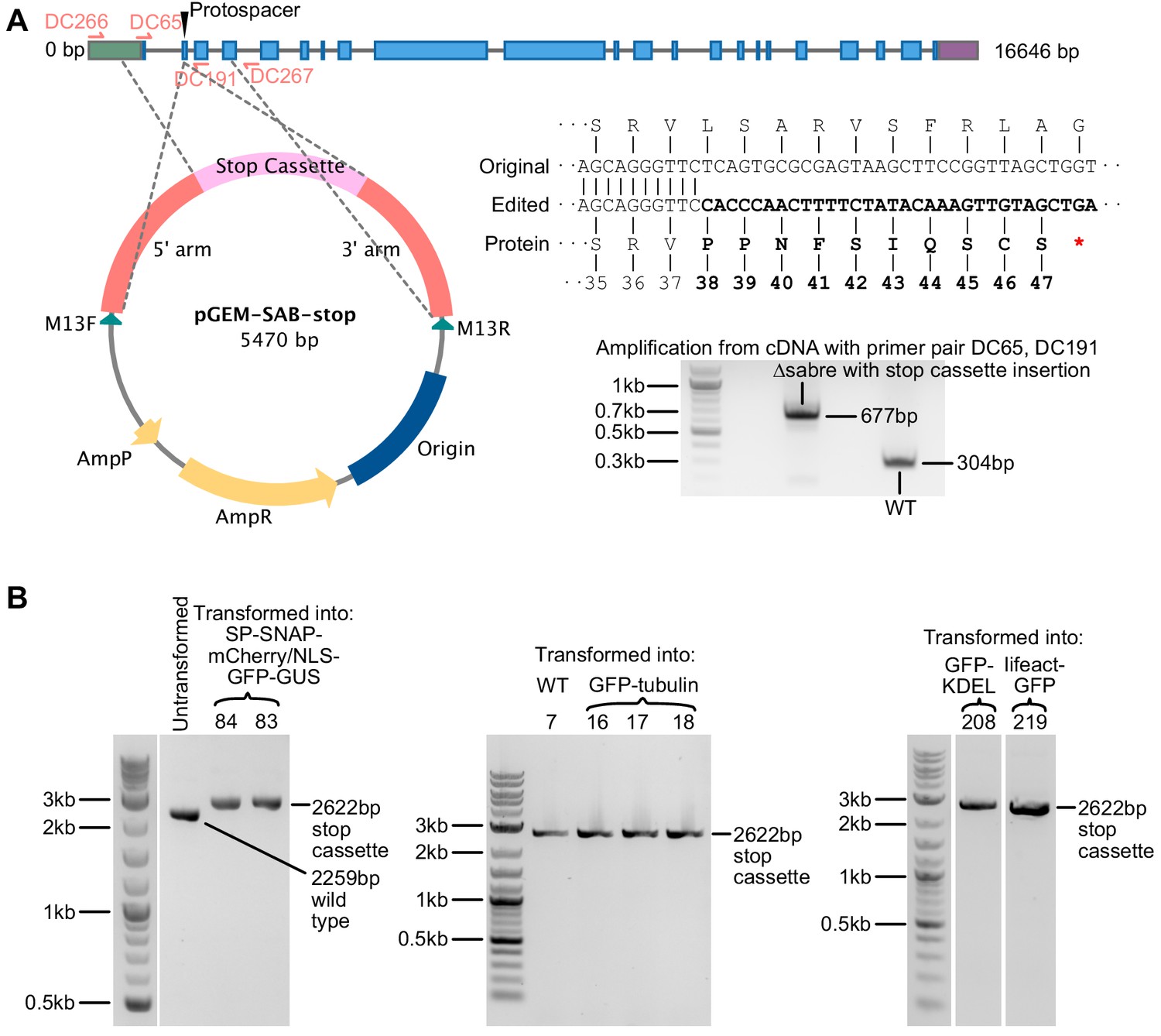
(A) Gene model of P. patens SABRE and scheme for generating the null mutation. Protospacer indicates the region targeted for double-stranded break and insertion of the stop cassette. Gray line, introns; green box, 5′UTR; purple box, 3′UTR; blue boxes, exons. Gray dashed lines extending from the plasmid map indicate the regions of homology. Original and edited DNA sequences near the insertion site are shown. Bold font indicates DNA sequences of inserted stop cassette and its translated protein that is different from the original sequence. Red asterisk indicates the premature stop codon. Gel image shows PCR amplification from cDNA made from total mRNA of ∆sabre and wild type plants. Cloning and sequencing the PCR amplicons shown in the gel confirmed that ∆sabre transcripts contained the expected mutation. (B) Gel images showing PCR products amplified from mutants isolated in a variety of different backgrounds with the homology-directed repair stop cassette insertion amplified by primer pairs DC266, DC267. An untransformed control is shown in the first gel. All insertions were validating by sequencing.
Figure 1—figure supplement 2
Early gametophore development.
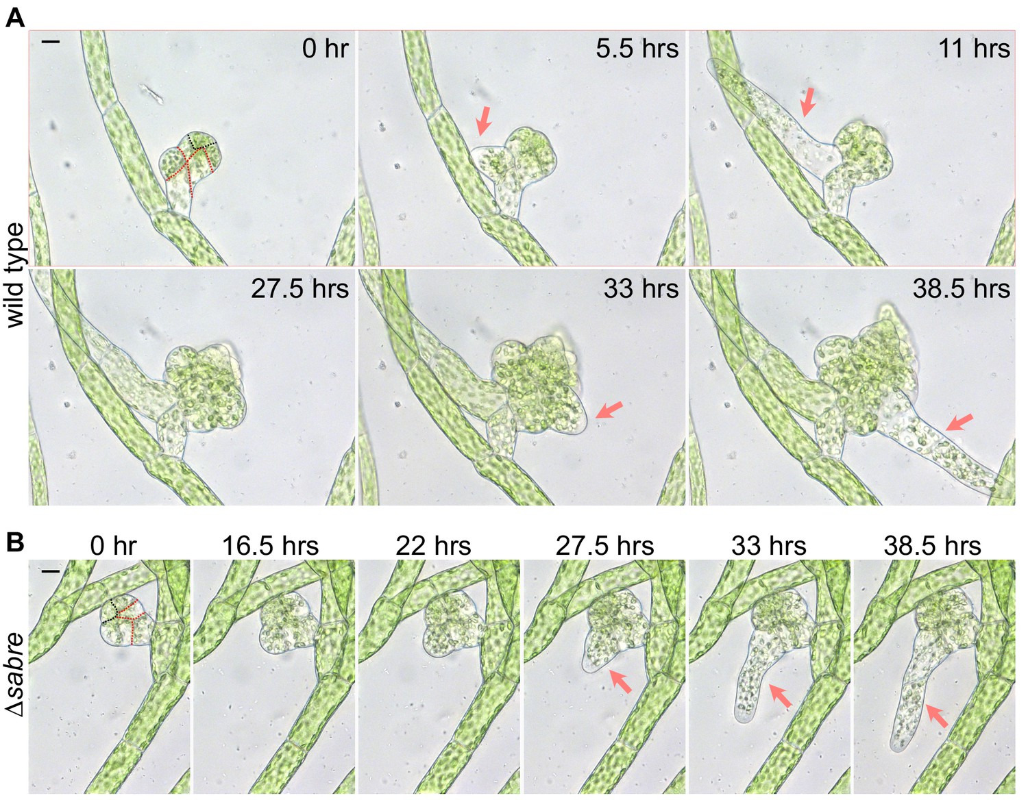
Gametophore initials (buds) from wild type (A) and ∆sabre (B). Both have undergone stereotypic divisions (dashed red lines) to produce the apical pyramidal stem cell (dashed black line). In wild type (A), two rhizoids (arrows) emerged from the base of the developing gametophore and elongated by polarized growth. Scale bar, 10 µm. A ∆sabre (B) gametophore of similar age to the wild type shown in (A) growing for the same period of time. The ∆sabre bud and rhizoid (arrows) grew significantly less than wild type. Scale bar, 10 µm. Also see Video 1.
Figure 2 with 1 supplement
Reduced cell expansion underlies small plant size in ∆sabre.
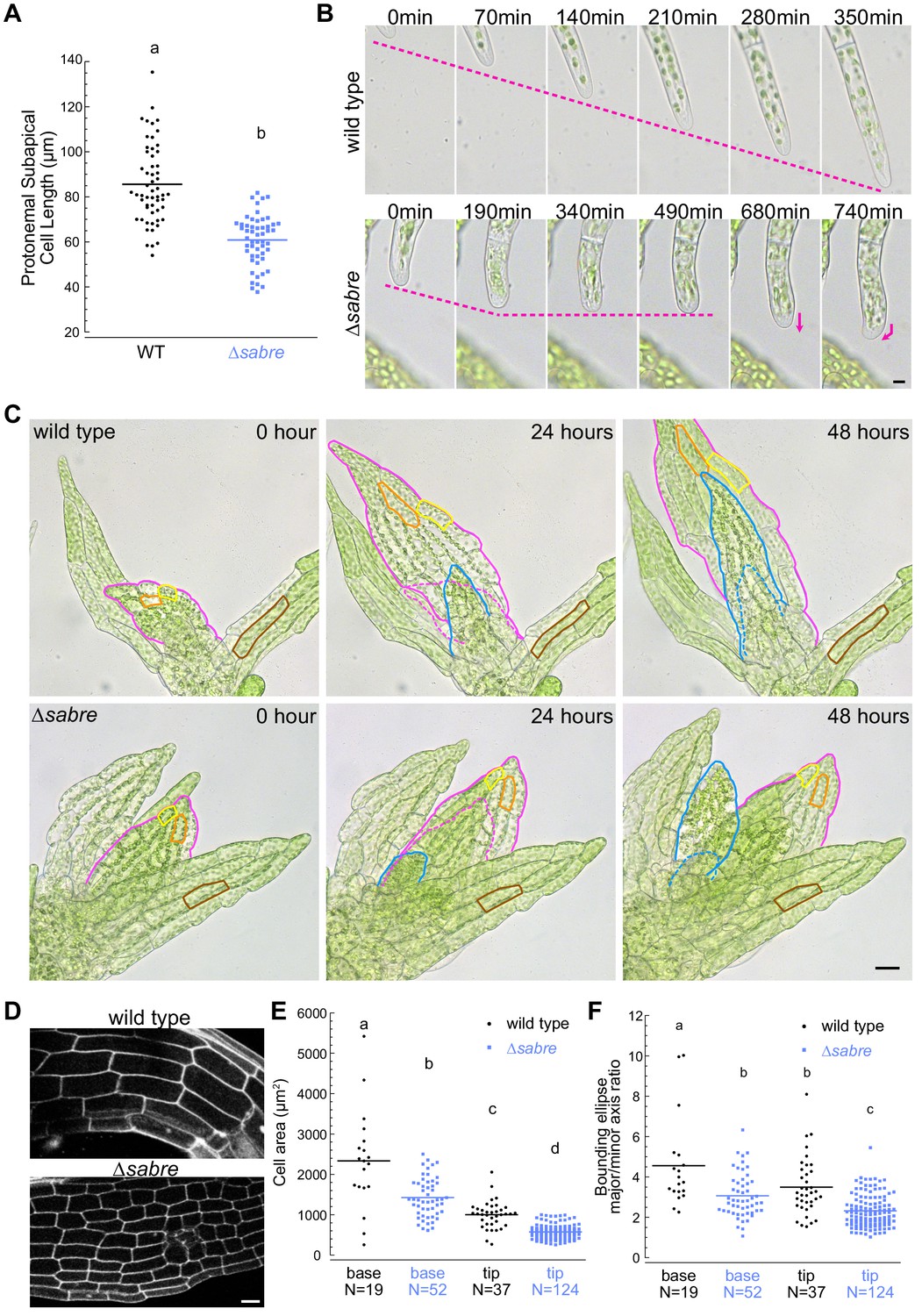
(A) Quantification of subapical cell length from 7-day-old plants regenerated from protoplasts. N = 56, wild type; N = 53, ∆sabre. Statistically significant different means were determined by Student’s t-test for unpaired data with equal variance, with p value indicated above the graph. (B) Brightfield time-lapse images for wild type (top) and ∆sabre protonemata (bottom). Scale bar, 5 µm. Magenta dashed lines indicate the apical positions of the cells. Magenta arrows indicate growth directionality. Also see Video 2. (C) Brightfield time-lapse imaging of gametophores growing in microfluidic imaging devices. Magenta and blue lines indicate example phyllids 1 and 2, respectively, that expanded during the imaging period. Dashed lines in corresponding colors indicate the phyllid outlined 24 hr before. Orange and yellow lines outline example cells that expanded during the imaging period. Brown lines highlight example cells in a mature phyllid that did not obviously increase in size. Scale bar, 20 µm. Also see Video 3. (D) Example confocal fluorescent images of phyllids stained with propidium iodide used for quantification in (E, F). Scale bar, 30 µm. (E) Quantification of phyllid cell area. Base and top indicate cells were located at the base or top of the phyllid. (F) Quantification of the ratio of major/minor axis of the bounding ellipse fitted to each cell. Number of cells in each category indicated under the graph. Letters indicate groups that are significantly different as determined by one-way ANOVA with Tukey’s HSD post-hoc test (α = 0.05). For statistical analysis details, see Supplementary file 1 for (E) and 5 for (F).
-
Figure 2—source data 1
Quantification of sub-apical cell length.
- https://cdn.elifesciences.org/articles/65166/elife-65166-fig2-data1-v2.xlsx
-
Figure 2—source data 2
Quantification of phyllid cell area and shape.
- https://cdn.elifesciences.org/articles/65166/elife-65166-fig2-data2-v2.xlsx
Figure 2—figure supplement 1
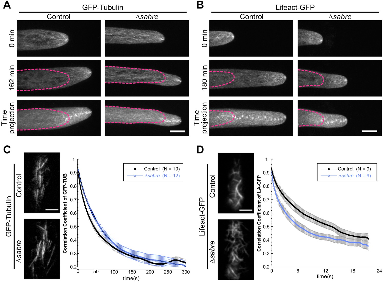
Organization and dynamics of actin and microtubule cytoskeletons in ∆sabre.
(A) Microtubule and (B) actin tip foci are not altered in ∆sabre. Images are maximum projections of confocal Z-stacks; the first and last frames from a time-lapse acquisition are shown. The time projection images are maximum projections of the 19 frames from the time lapse. The magenta dashed lines indicate the outlines of the cells in the first time point. Scale bar, 3 µm. (C, D) Quantification of cortical microtubule (C) and actin (D) dynamics. Representative images are single frames of a variable angle epifluorescence microscopy time-lapse acquisition showing the overall cortical cytoskeleton organization. Graphs depict the correlation coefficient between images over all possible temporal spacings (time interval, X axis). Each data point is the average of several cells; the number of cells for each category is indicated in the graph legends. Scale bars, 3 µm. Error bar, standard error of the mean.
-
Figure 2—figure supplement 1—source data 1
Quantification of cortical microtubule dynamics.
- https://cdn.elifesciences.org/articles/65166/elife-65166-fig2-figsupp1-data1-v2.xlsx
-
Figure 2—figure supplement 1—source data 2
Quantification of cortical actin dynamics.
- https://cdn.elifesciences.org/articles/65166/elife-65166-fig2-figsupp1-data2-v2.xlsx
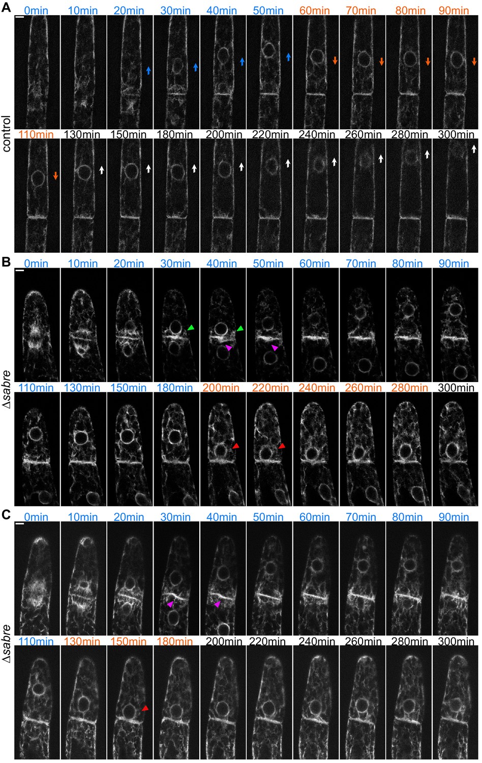
Figure 3 with 1 supplement
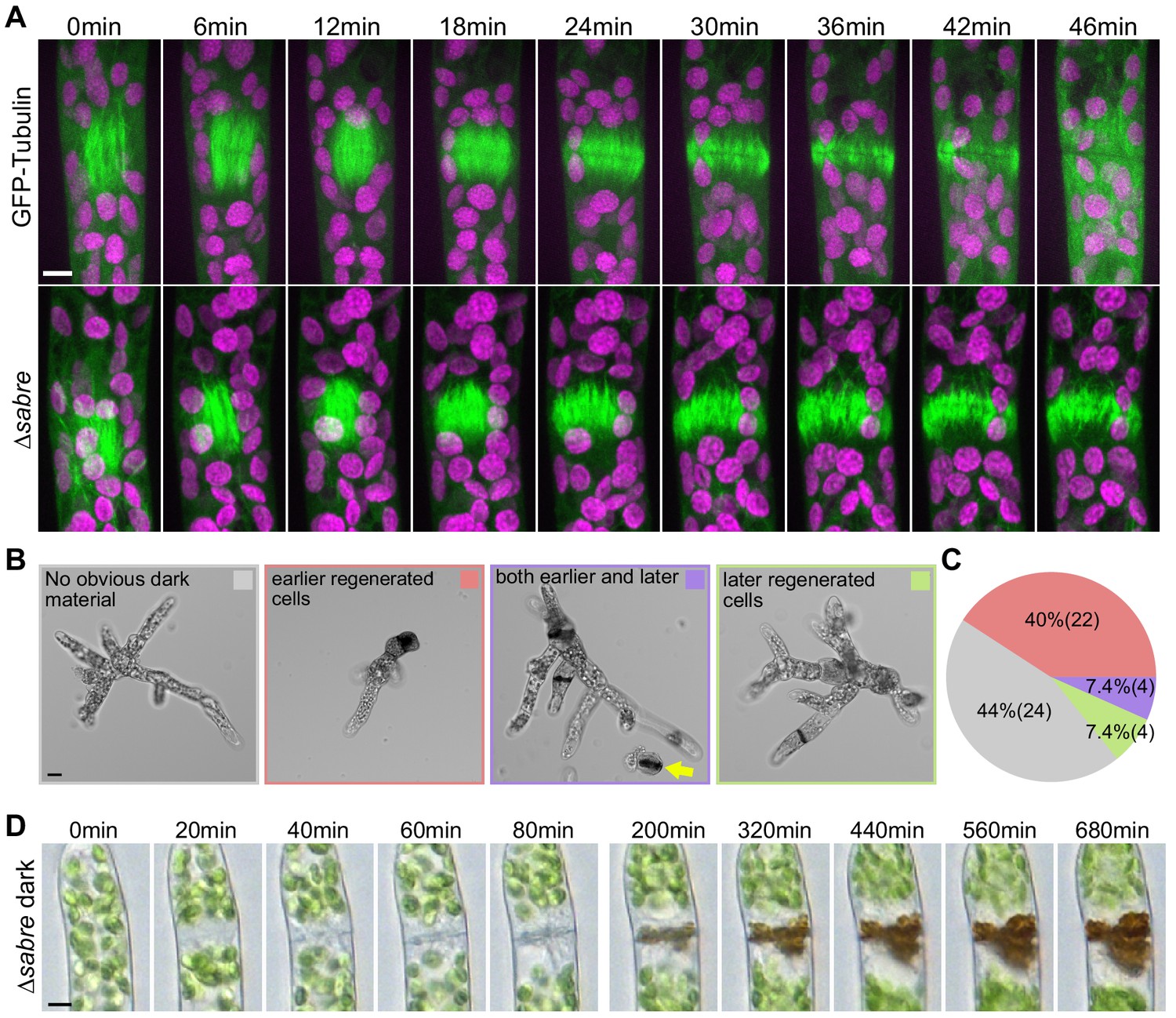
Delays in disassembling phragmoplast microtubules and quantification of cytokinesis failures during protonemal development.
(A) Time-lapse imaging of phragmoplast microtubules. GFP-tubulin (green) and chlorophyll autofluorescence (magenta) are shown. First frames (0 min) occur within 2 min of nuclear envelope breakdown. Scale bar, 5 µm. Also see Video 4. (B) Representative images depicting brown material deposition near cell plates in 7-day-old plants regenerated from protoplasts. Colored frames correspond to categories quantified in (C). Yellow arrow indicates an example of a dead protoplast containing dark brown material at the first cell division site, resulting in the failure to regenerate. Scale bar, 20 µm. (C) Frequency of brown material deposits at different developmental stages (marked by cell shape and position in regenerated plant). Numbers in parentheses indicate numbers of plants. (D) Brightfield time-lapse extended-depth-of-focus images of brown material deposition in a cell that underwent cell division. Also see Video 5. Scale bar, 5 µm.
Figure 3—figure supplement 1
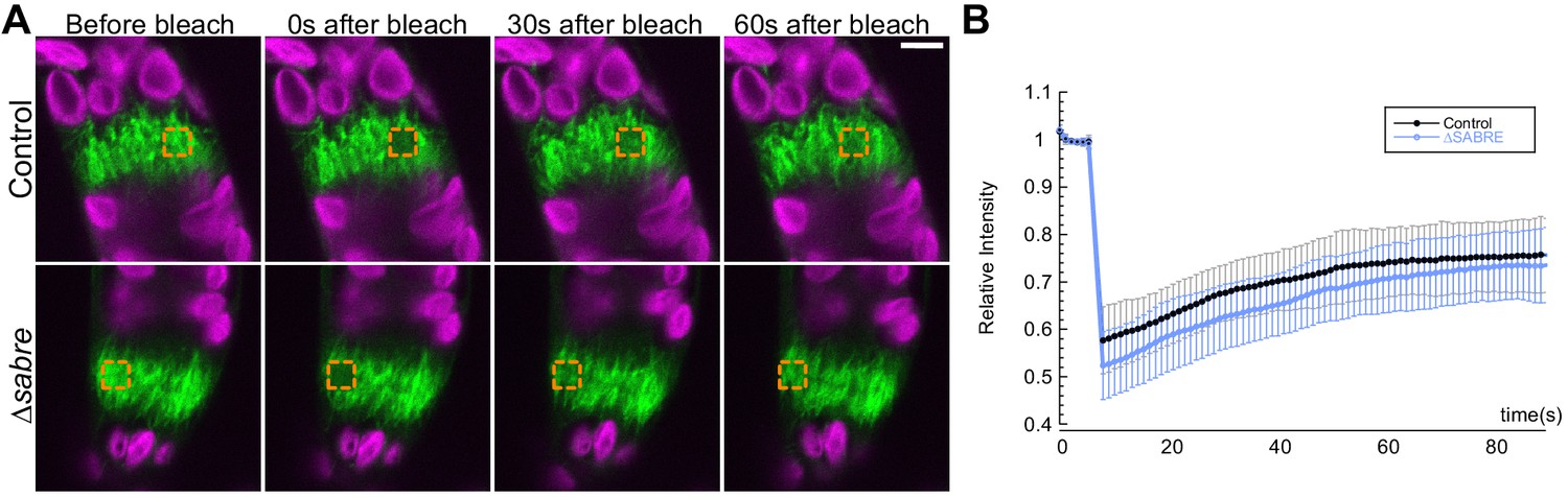
Phragmoplast microtubule dynamics are not altered in ∆sabre.
(A) Photobleaching of phragmoplast microtubules labeled with GFP-tubulin. Orange square indicates photobleached region. GFP-tubulin (green) and chlorophyll autofluorescence (magenta) are shown. Scale bare, 5 µm. (B) Relative intensity is plotted against time to show the recovery rate of fluorescence over the following 1.5 min after the bleaching event. Error bars represent standard deviation.
-
Figure 3—figure supplement 1—source data 1
Recovery rate of fluorescence for 1.5 minutes after the bleaching event.
- https://cdn.elifesciences.org/articles/65166/elife-65166-fig3-figsupp1-data1-v2.xlsx
Figure 4 with 3 supplements
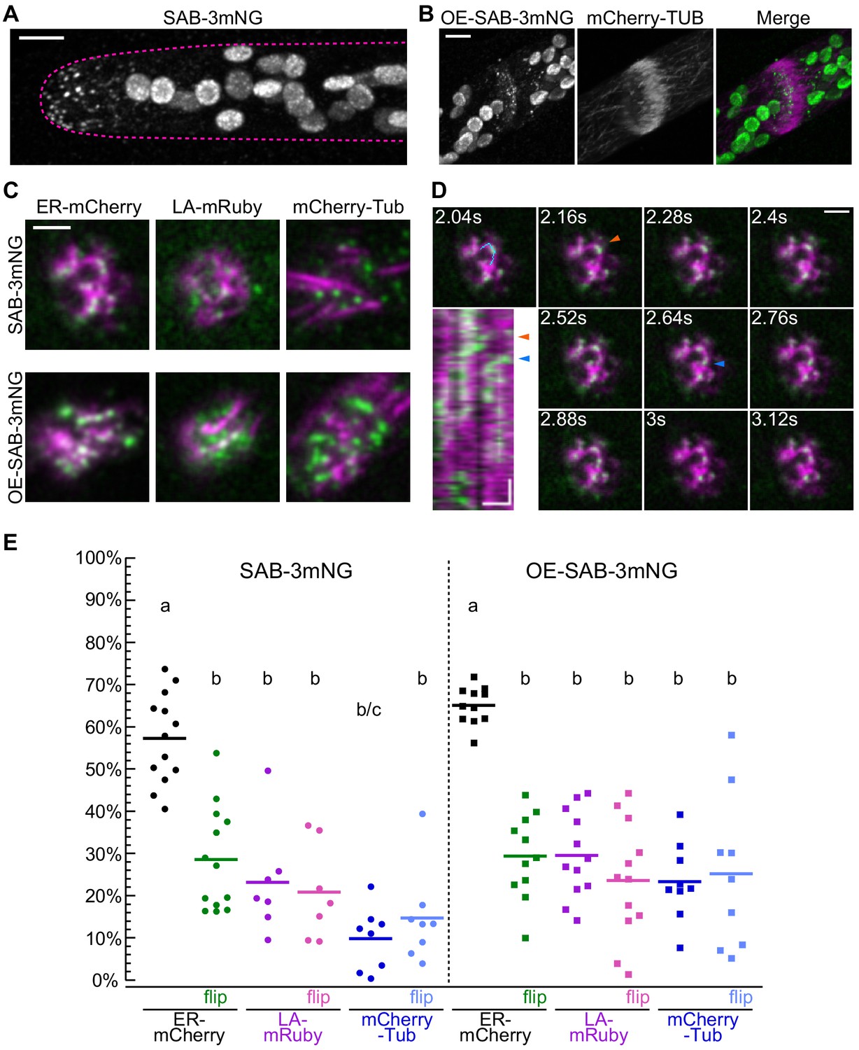
Localization of SABRE revealed by tagging SABRE at the C-terminus with three tandem mNeonGreen proteins.
(A) SABRE-3mNeonGreen (SAB-3mNG) forms small puncta at the cell cortex that are more numerous near the tip of a growing apical cell. Image is a maximum projection of a deconvolved confocal Z-stack. Magenta dashed line indicates the outline of the cell. Scale bar, 5 µm. (B) Deconvolved confocal images of SABRE localization at the maturing cell plate. Scale bar, 5 µm. SAB-3mNG (green in merge) and mCherry-tubulin (magenta in merge) are shown. Large globular structures are chloroplasts, which autofluorescence in the mNeonGreen channel under these imaging conditions. (C) Variable angle epifluorescence microscopy (VAEM) images of SAB-3mNG (green) with mCherry-tubulin (mCherry-Tub), Lifeact-mRuby (LA-mRuby), and mCherry-KDEL (ER-mCherry) (magenta). Representative images are the first frame of a VAEM time-lapse acquisition. Scale bar, 2 µm. Also see Video 6. (D) VAEM time-lapse acquisition showing SAB-3mNG (green) moving along an endoplasmic reticulum (ER) tubule (magenta). Scale bar, 2 µm. Kymograph was generated using the cyan line drawn in the 2.04 s frame. Orange and blue arrowheads indicate two events when a SAB-3mNG puncta starts to move along the ER tubule. Horizontal scale bar, 1 µm. Vertical scale bar, 1.2 s. (E) Quantification of the fraction of SABRE area that overlapped with ER, actin, or microtubules for SAB-3mNG (left) and OE-SAB-3mNG (right). The area fraction is shown as a percentage for each category, with each data point representing the average of the first 50 frames of a time-lapse acquisition (120 ms interval) for one cell. For SAB-3mNG: N = 13, ER-mCherry; N = 7, LA-mRuby; N = 8, mCherry-Tub. For OE-SAB-3mNG: N = 11, ER-mCherry; N = 12, LA-mRuby; N = 9, mCherry-Tub. Letters indicate groups with significantly different means as determined by ANOVA with a Tukey’s HSD all-pair comparison post-hoc test (α = 0.05). For statistical analysis details, see Supplementary file 1.
-
Figure 4—source data 1
Quantification of the fraction of SABRE area that overlapped with ER, actin, or microtubules.
- https://cdn.elifesciences.org/articles/65166/elife-65166-fig4-data1-v2.xlsx
Figure 4—figure supplement 1
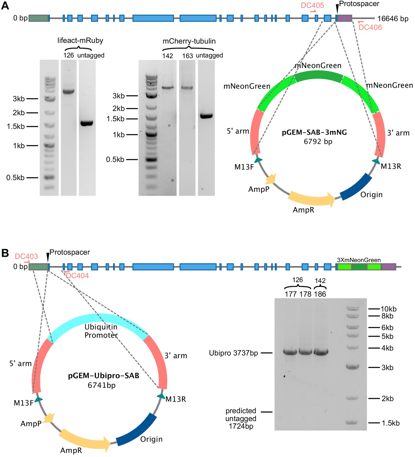
Model for generating SABRE-3mNG tag and overexpression with maize ubiquitin promoter.
(A, B) Generating (A) 3mNG tag at C terminus and (B) inserting maize ubiquitin promoter at N terminus of SABRE. Protospacer indicates the region targeted for double-stranded break. Grey lines, introns; green box, 5′UTR; purple box, 3′UTR; blue boxes, exons. Gray dashed lines extending from the plasmid maps indicate the regions of homology. Gel images shows PCR products amplified from transformed plants amplified by primer pairs DC405, DC406 for (A), and DC403, DC404 for (B). All insertions were validating by sequencing.
Figure 4—figure supplement 2

C-terminal tagging and overexpression of SABRE does not influence protein function.
(A) Quantification of plant area for the indicated genotypes of 7-day-old plants regenerated from protoplasts. Plant area was normalized to wild type. N = 20, wild type; N = 41, SAB-3GFP; N = 41, LA-mRuby; N = 44, SAB-3mNG/LA-mRuby; N = 43, mCherry-Tub; N = 40, SAB-3mNG/mCherry-Tub. Letters indicate groups with significantly different means as determined by ANOVA with a Tukey’s HSD all-pair comparison post-hoc test (α = 0.05). For statistical analysis details, see Supplementary file 1. (B) Comparison of SAB-3mNG and OE-SAB-3mNG plant area. Plant area was normalized to SAB-3mNG. N = 15, SAB-3mNG; N = 20, OE-SAB-3mNG. A Student’s t-test for unpaired data with equal variance was performed; p value indicated above the graph. (Right) Representative images of 7-day-old plants regenerated from protoplasts of the indicated genotype. Scale bar, 100 µm. (C) Example images comparing the density of SAB-3mNG and OE-SAB-3mNG. Magenta dashed lines label the cell outlines. Scale bar, 3 µm. (D) Representative images showing mutation of SABRE by inserting the stop cassette into its genomic locus eliminated the fluorescence of the fluorescent fusion protein. Pictures are maximum projections of deconvolved confocal Z-stack images covering the entire cell volume.
-
Figure 4—figure supplement 2—source data 1
Quantification of plant area.
- https://cdn.elifesciences.org/articles/65166/elife-65166-fig4-figsupp2-data1-v2.xlsx
Figure 4—figure supplement 3
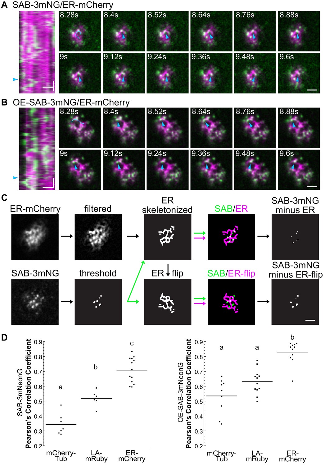
SABRE forms dynamic puncta that were associated with the endoplasmic reticulum (ER).
(A, B) Examples of SABRE dots moving along ER tubules in SAB-3mNG (A) and OE-SAB-3mNG (B). Images are from variable angle epifluorescence microscopy (VAEM) time-lapse acquisitions taken every 120 ms. Blue arrowheads indicate the moving dot along an ER tubule. Scale bar, 2 µm. Kymographs on the left were generated from the blue trace indicated in the 8.28 s frames. Vertical scale bars, 1.2 s. Horizontal scale bars, 2 µm. (C). Illustration of quantification method to calculate the area of SABRE overlapping with ER, actin, or microtubules, using ER as an example. Scale bar, 2 µm. (D) Quantification of SAB-3mNG (left) and OE-SAB-3mNG (right) co-localization with markers shown in Figure 4C. Pearson’s correlation coefficient from the first 10 frames of a VAEM time-lapse acquisition was obtained from NIS-Elements. The average correlation coefficient for each cell is plotted. For SAB-3mNG: N = 8, mCherry-Tub; N = 7, LA-mRuby; N = 13, ER-mCherry. For OE-SAB-3mNG: N = 9, mCherry-Tub; N = 12, LA-mRuby; N = 11, ER-mCherry. Letters indicate groups with significantly different means as determined by ANOVA with a Tukey’s HSD all-pair comparison post-hoc test (α = 0.05). For statistical analysis details, see Supplementary file 1.
-
Figure 4—figure supplement 3—source data 1
Pearson's correlation coefficients of SABRE with ER, actin or microtubules.
- https://cdn.elifesciences.org/articles/65166/elife-65166-fig4-figsupp3-data1-v2.xlsx
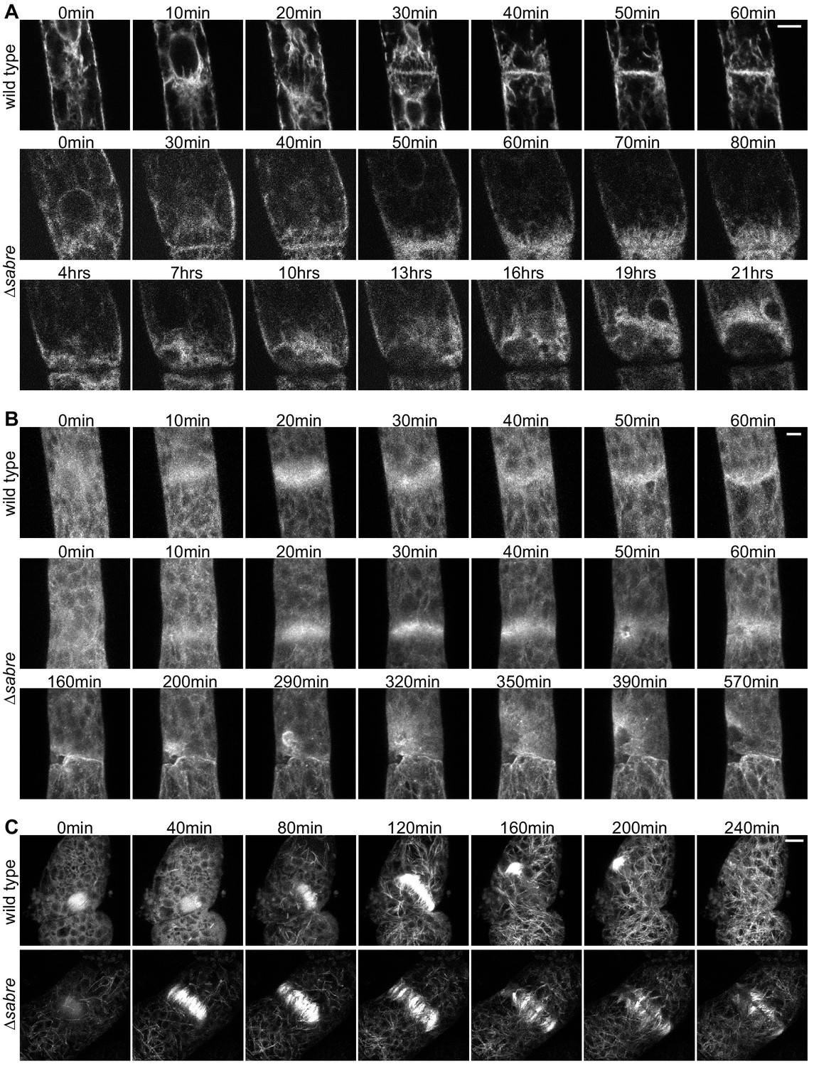
Figure 5 with 1 supplement
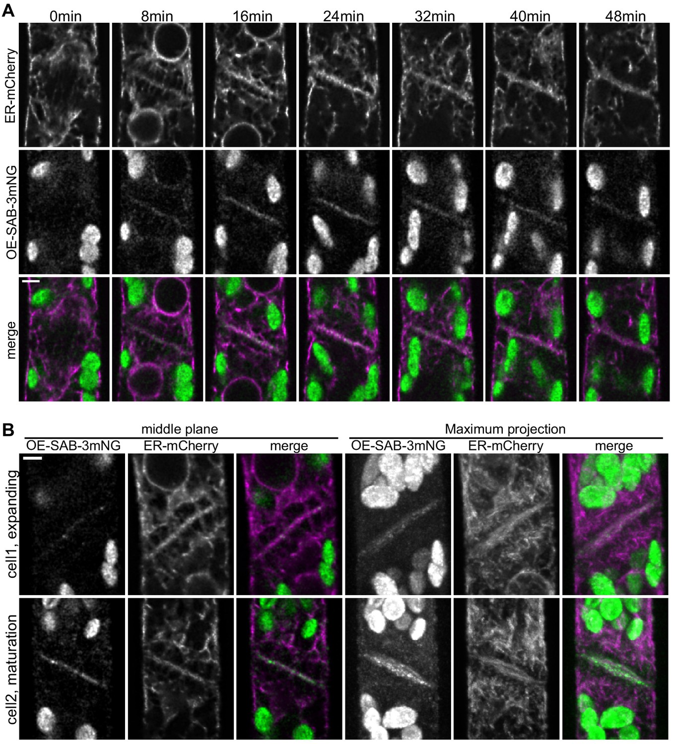
SABRE and endoplasmic reticulum (ER) accumulate on the nascent cell plate during cell plate maturation.
(A) Deconvolved confocal images of OE-SAB-3mNG (green in merge) and mCherry-tubulin (magenta in merge) during cell division. Individual frames are medial focal planes of the cell. Scale bar, 3 µm. Also see Video 7. (B) Two representative cells with ER-mCherry (magenta in merge) and OE-SAB-3mNG (green in merge) showing the difference in the accumulation of SABRE and ER during cell plate expansion and maturation. Scale bar, 3 µm.
Figure 5—figure supplement 1
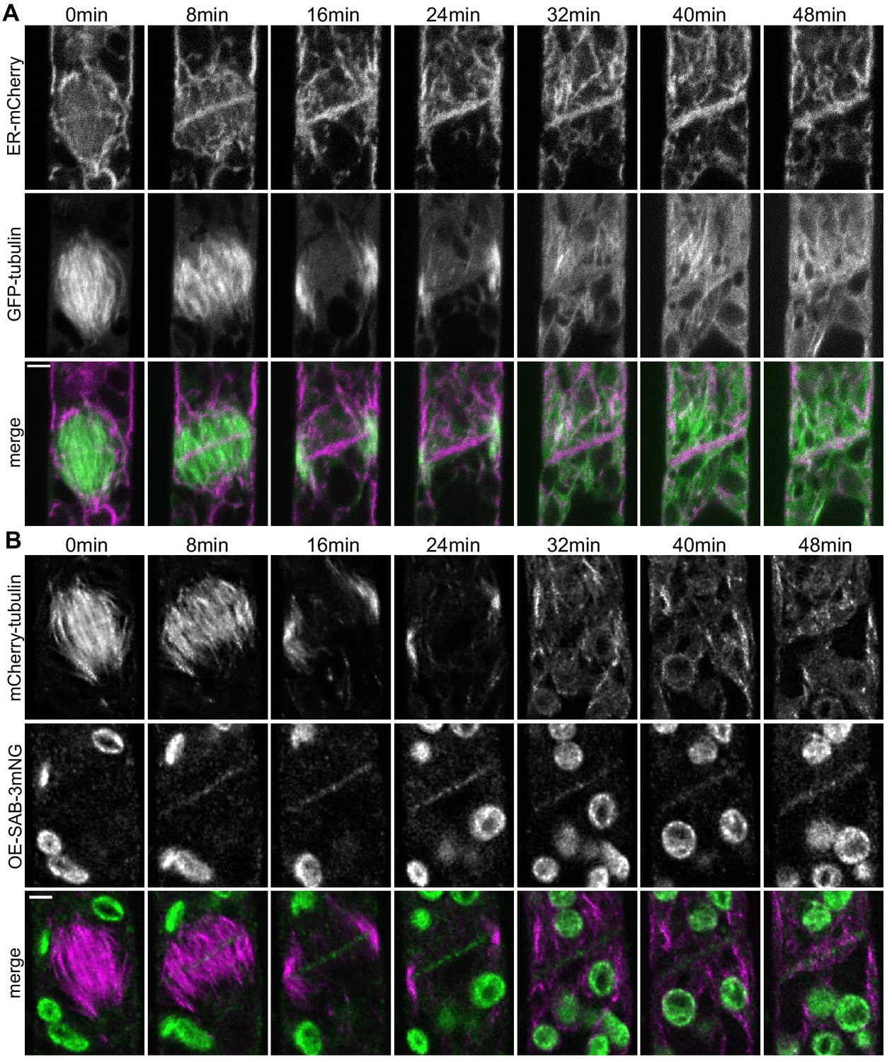
Timing of endoplasmic reticulum (ER), microtubule, and SABRE localization during cell plate formation.
(A) Confocal images of GFP-tubulin (green in merge) and ER-mCherry (magenta in merge) during cell division in a wild type cell. Scale bar, 3 µm. Also see Video 7. (B) Deconvolved images of OE-SAB-3mNG (green in merge) and mCherry-tubulin (magenta in merge) during cell division. Scale bar, 3 µm. Also see Video 7.
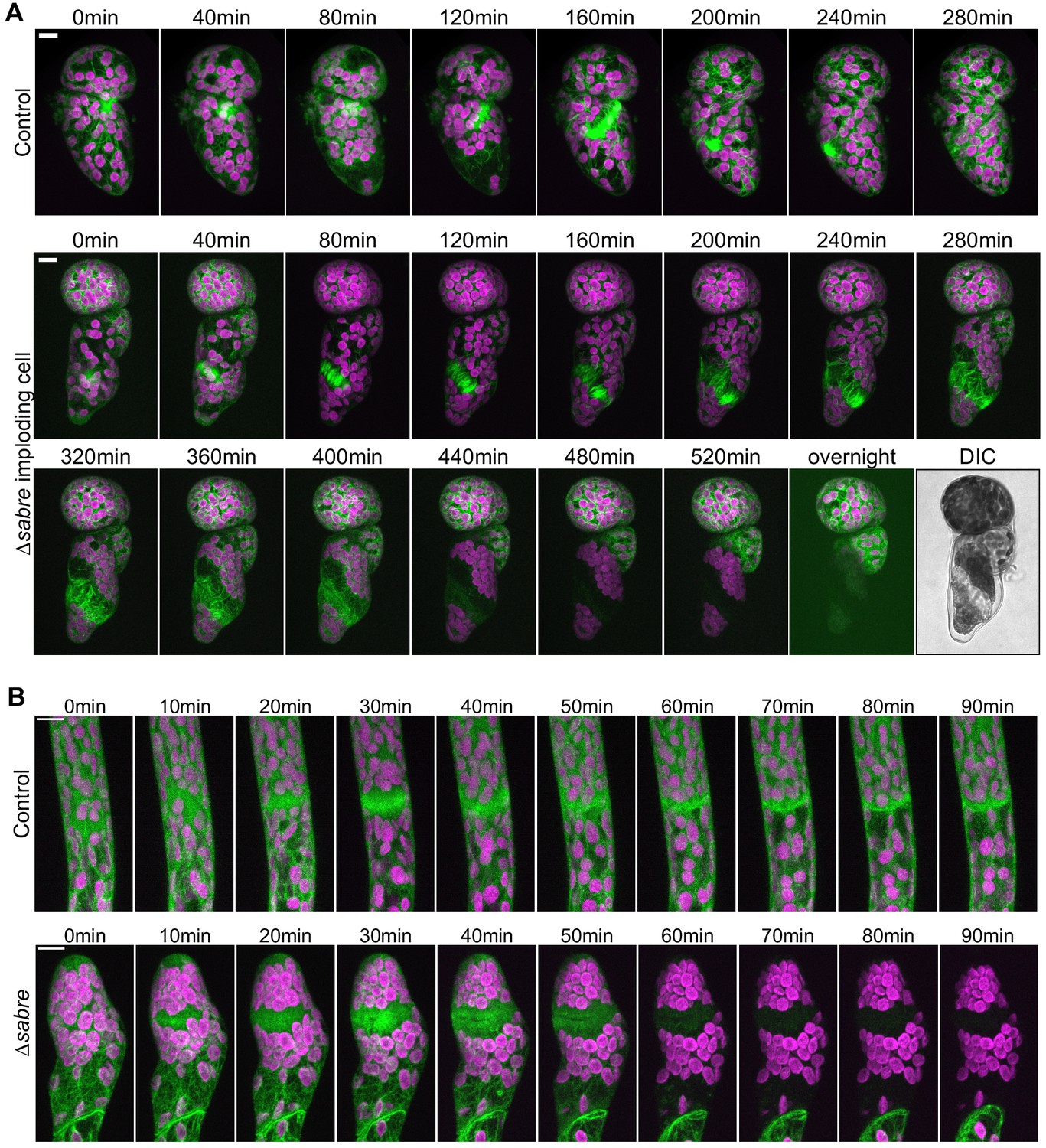
Figure 6 with 1 supplement
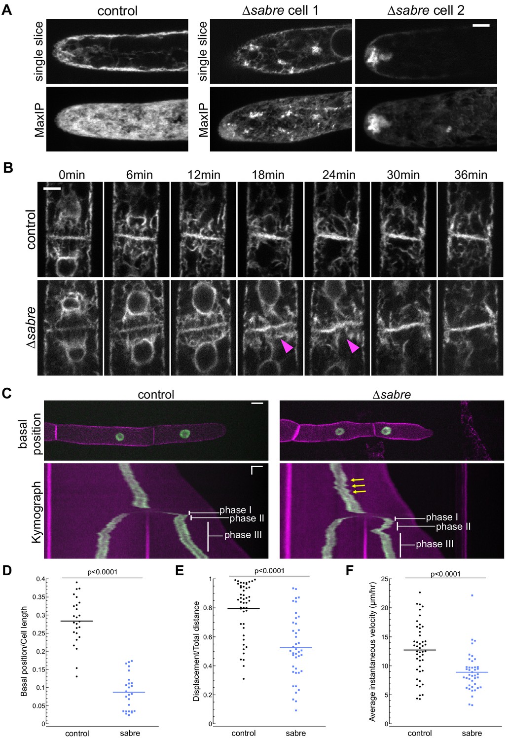
SABRE influences the endoplasmic reticulum (ER) and nuclear migration.
(A) Example images from one control cell and two ∆sabre cells expressing SP-GFP-KDEL, which localizes to the ER lumen. Top: single focal plane. Bottom: maximum projection of confocal Z-stacks. Scale bar, 5 µm. Also see Video 8. (B) ER during cell division in wild type and ∆sabre cells. First frame is within 3 min of nuclear envelop reformation. ER buckles at the nascent cell plate in ∆sabre (magenta arrowheads). Scale bar, 5 µm. Also see Video 9. (C) Top panel: representative images of control and ∆sabre cells when the nucleus in the tip cell is closest to the new cell plate (basal position). NLS-GFP-GUS (green) accumulates in the nucleus, and SNAP-TM-mCherry (magenta) labels the plasma membrane. Scale bar, 10 µm. Bottom panel: kymograph created by drawing a line in the middle of the cell along the growth axis. Horizontal scale bar, 10 µm. Vertical scale bar, 1 hr. (D) Distance of the nucleus in the apical cell to the newly formed cell plate when it is at the basal position normalized to cell length. N = 25. (E) Quantification of linearity of nuclear movement during apical moving phases (I and III). Linearity determined by the ratio of total distance traveled divided by total linear displacement. Nuclear movement was tracked with TrackMate plugin in Fiji generating distance and displacement of nucleus. N = 46, control; N = 41, ∆sabre. (F) Quantification of nuclear velocity for the same cells and migration phases in (E). Average instantaneous velocity (µm/hour) was determined by dividing the total distance traveled by the time. Statistical analyses for (D–F) were performed using Student's t-test for unpaired data with equal variance, with p value indicated above the graphs. Also see Video 11.
-
Figure 6—source data 1
Quantification of nuclear movement.
- https://cdn.elifesciences.org/articles/65166/elife-65166-fig6-data1-v2.xlsx
Figure 6—figure supplement 1
SABRE influences the endoplasmic reticulum (ER), impacting nuclear movement and ER morphology at the nascent cell plate.
(A) ER behavior in control cells during cell plate formation and nuclear migration after mitosis. Time points and arrows in blue indicate cell division and the initial apical nuclear movement (phase I), orange indicates basal nuclear movement (phase II), and black text accompanied with white arrows in the image indicates apical nuclear movement with polarized growth (phase III). (B, C) ER behavior in two example ∆sabre cells. As in (A), the initial time points are within 10 min of nuclear envelope formation. Magenta arrowheads indicate ER buckling at the nascent cell plate. Red arrowheads indicate exaggerated basal nuclear movement. Green arrowheads indicate abnormally close contact between the nucleus and the nascent cell plate during the phase I apical movement. Scale bars, 5 µm. Also see Video 10.
Figure 7 with 1 supplement
Behavior of endoplasmic reticulum (ER), actin, and microtubules during cytokinesis failures in ∆sabre.
Single focal planes from confocal images of (A) ER labeled with SP-GFP-KDEL, maximum projection of confocal Z-stacks of (B) actin labeled with Lifeact-GFP, and (C) microtubules labeled with GFP-tubulin in wild type and ∆sabre cells that accumulate brown material during cell division. (A) Between 0 and 20 min, a phragmoplast formed. At 30 min, the ∆sabre phragmoplast failed to mature and brown material deposition gradually occurred over the following hours. Scale bar, 6 µm. (B) Scale bar, 5 µm. (C) Scale bar, 10 µm. Also see Video 12.
Figure 7—figure supplement 1
Phragmoplast microtubule and actin behavior during cytokinesis failures in ∆sabre that resulted in cell lysis during cell division with no brown material deposition.
(A) Time-lapse imaging of GFP-tubulin (green) and chlorophyll autofluorescence (magenta) in 4-day-old plants regenerated from protoplasts. Images are maximum projections of confocal Z-stacks. Top: a control cell dividing successfully. Bottom: a ∆sabre cell exhibiting phragmoplast microtubule disorganization and rapid cell lysis. Differential interference contrast image in (B) depicts the dead cell at the end of the movie. Scale bars, 10 µm. (B) Actin labeled with Lifeact-GFP (green) and chlorophyll autofluorescence (magenta) during cell division. Scale bars, 10 µm. Top: a control cell dividing successfully. Bottom: a ∆sabre cell that lysed during cell plate formation.
Figure 8
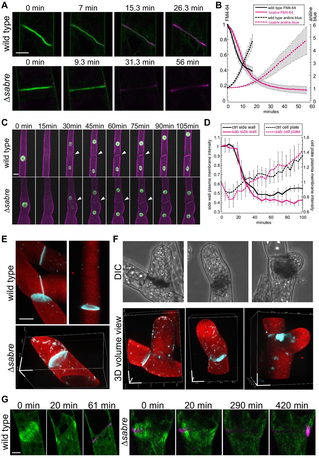
Aniline blue deposition is altered in ∆sabre.
(A) Time lapse of FM4-64 (green) and aniline blue (magenta) showing aniline blue staining the cell plate after FM4-64 staining diminishes. Also see Video 13. (B) Quantification of FM4-64 and aniline blue at the developing cell plate over time. Intensity is measured by drawing a 15-pixel wide curved line along the developing cell plate and measuring the mean intensity value. Each data point is the average of N = 6 cells for each category. Intensity is normalized to the starting point of the time lapse – the moment when FM4-64 is the strongest and no aniline blue stain accumulates. Error bars, standard error of the mean. (C) Time lapse of membrane marker SNAP-TM-mCherry (magenta) and nuclear marker NLS-GFP-GUS (green) during cell division. A 0 min frame depicts the last time point (within 5 min) before nuclear envelope breaks down. Also see Video 11. (D) Quantification of signal intensity in (C). A region of interest of 6–10 µm2 was manually drawn at the side wall where membrane fusion occurs and at the middle of the cell plate, respectively, and mean intensity was measured for those two regions of interests and plotted against time. Each data point is the average of N = 6 cells for each category. Error bars, standard error of the mean. (E) Example 3D images of normal mature cell plates stained with aniline blue (cyan) and fast scarlet (F2B) (red) to outline the cell wall. (F) Examples of different aniline blue staining patterns in ∆sabre mutants containing brown material. Left, weak stain; middle, partial stain; and right, large chunk near the cell plate. Scale bars, 10 µm. (G) Time lapse showing aniline blue staining (magenta) in a wild type cell and a ∆sabre cell with brown material. Images are maximum projections of deconvolved confocal Z-stacks. Microtubules labeled with GFP-tubulin are shown in green. Scale bar, 5 µm. Also see Video 14.
-
Figure 8—source data 1
Measurement of FM4-64 and aniline blue intensities.
- https://cdn.elifesciences.org/articles/65166/elife-65166-fig8-data1-v2.xlsx
Videos
Video 1
Early gametophore development in wild type and ∆sabre.
Each frame is an extended-depth-of-focus image generated from a brightfield Z-stack taken every 15 min. Scale bar, 10 µm. Video is playing at 10 fps.
Video 2
SABRE influences polarized growth in protonemata.
Brightfield images were taken every 10 min. Scale bar, 5 µm. Video is playing at 10 fps.
Video 3
SABRE influences diffused growth in gametophores.
Extended-depth-of-focus images of brightfield Z-stacks taken every hour. Scale bar, 20 µm. Video is playing at 5 fps.
Video 4
Delays in disassembling phragmoplast microtubules in ∆sabre mutant.
Images are maximum projections of confocal Z stacks of GFP-tubulin (green) and chlorophyll autofluorescence (magenta) in control and ∆sabre cells acquired every 2 min. Video is playing at 5 fps. Scale bar, 10 µm.
Video 5
Brown material deposition in ∆sabre occurs during cell plate formation.
Each frame is a brightfield extended-depth-of-focus image taken every 10 min. Video is playing at 8 fps. Scale bar, 5 µm.
Video 6
Representative variable angle epifluorescence microscopy (VAEM) time-lapse acquisitions showing localization of SABRE with microtubules, actin, or endoplasmic reticulum (ER).
SAB-3mNG or OE-SAB-3mNG (green), and ER (mCherry-KDEL), microtubules (mCherry-tubulin) or actin (LA-mRuby) (magenta) are shown. Time lapse acquired every 120 ms. Video is playing at 10 fps. Scale bar, 2 µm.
Video 7
SABRE accumulation correlates with endoplasmic reticulum (ER) localization at the phragmoplast and both signals accumulated during later stages of cell division.
Images are single focal planes in the medial section of the cell. OE-SAB-3mNB (SAB), mCherry/GFP-tubulin (MT), and ER-mCherry (ER). Frame interval is 1 min. Video is playing at 5 fps. Scale bar, 3 µm.
Video 8
∆sabre exhibits bright endoplasmic reticulum aggregates in the cytoplasm.
Images are single focal planes in the medial section and maximum projections of confocal Z-stacks of the cells showing SP-GFP-KDEL in control and ∆sabre. Confocal Z-stacks acquired every 10 min. Video is playing at 4 fps. Scale bar, 5 µm.
Video 9
Endoplasmic reticulum buckles during cell plate formation in ∆sabre.
Each frame is a single focal plane in the medial section of the cell, taken every 3 min. Magenta arrow indicates buckling. Video is playing at 5 fps. Scale bar, 5 µm.
Video 10
Time-lapse imaging showing exaggerated nuclear basal migration in relation to phragmoplast endoplasmic reticulum (ER) buckling during cell plate formation.
∆sabre cell 1 showed delayed apical nuclear movement in phase I and exaggerated basal movement in phase II. ∆sabre cell 2 showed only exaggerated basal movement in phase II. Both cells exhibited ER buckling at the cell plate. Images are single confocal images taken every 10 min. Video is playing at 4 fps. Scale bar, 5 µm.
Video 11
Nuclear movement during tip growth and cell division.
Blue traces represent the mother nuclei, and red and green traces represent the daughter nuclei in the apical and subapical cells, respectively. Nuclei are shown in green or gray with colored tracks, and plasma membrane shown in magenta. The column on the far right depicts a ∆sabre cell showing impaired forward nuclear movement before cell division and exaggerated basal nuclear movement after cell division. The nucleus moved basally all the way to the newly formed cell plate, appearing to smash into the cell plate, with an evident change in nuclear shape. The nucleus flattens out when in contact with the cell plate, observed at 510–525 min. Video is a maximum projection of confocal Z-stacks taken every 5 min. Video is playing at 8 fps. Scale bar, 10 µm.
Video 12
Endoplasmic reticulum (ER), actin, and microtubule behavior during brown material deposition and cell division failure in ∆sabre.
Single focal plane of ER (SP-GFP-KDEL), maximum projection of actin (Lifeact-GFP), and microtubules (GFP-tubulin) are shown. Time-lapse imaging was acquired every 10 min. Video is playing at 5 fps. Scale bar, 10 µm.
Video 13
Aniline blue and FM4-64 staining at developing cell plate.
Green, FM4-64; magenta, aniline blue. Images are medial sections from dividing cells. Scale bar, 5 µm. Video is playing at 8 fps.
Video 14
Aniline blue staining during normal division and cytokinesis failure in ∆sabre.
Images are maximum projections of deconvolved confocal Z-stacks taken every 10 min. Green, microtubule; magenta, aniline blue. Scale bar, 10 µm. Video is playing at 5 fps.
Tables
Key resources table
| Reagent type (species) or resource | Designation | Source or reference | Identifiers | Additional information |
|---|---|---|---|---|
| Gene (Physcomitrium patens) | SABRE | Phytozome | Pp3c12_12980 | Gene of interest in this study |
| Other | Calcofluor white | Sigma Aldrich | 18909 | 0.1 mg/mL dissolved in Hoagland’s media |
| Other | Propidium iodide | Sigma Aldrich | 81845 | 15 µg/mL dissolved in Hoagland’s media |
| Other | FM-4-64 | Invitrogen | T3166 | 15 µM dissolved in Hoagland’s media |
| Other | Aniline blue | Fisher Scientific | 28631-66-5 | 20 µg/mL dissolved in Hoagland’s media |
| Other | Fast Scarlet | Sigma Aldrich | R320919 | 50 µg/mL dissolved in Hoagland’s media |
| Sequenced-based reagent | DC65 | This paper | PCR primers | caccATGGAGGTTACACCTGAC |
| Sequenced-based reagent | DC164 | This paper | Protospacer primer | ccatTCAGTGCGCGAGTAAGCTTC |
| Sequenced-based reagent | DC164 | This paper | Protospacer primers | aaacGAAGCTTACTCGCGCACTGA |
| Sequenced-based reagent | DC175 | This paper | PCR primers | GGGGACAAGTTTGTACAAAAAAGCAGGCTTAGTGATTGAGCAACAGCTATTGC |
| Sequenced-based reagent | DC176 | This paper | PCR primers | GGGGACAACTTTGTATAGAAAAGTTGGGTGGAACCCTGCTGGCTATC |
| Sequenced-based reagent | DC177 | This paper | PCR primers | GGGGACAACTTTGTATAATAAAGTTGTAGCTTCCGGTTAGCTGGT |
| Sequenced-based reagent | DC168 | This paper | PCR primers | GGGGACCACTTTGTACAAGAAAGCTGGGTTCTGCTGGATACAGTGAGATG |
| Sequenced-based reagent | DC265 | This paper | Sequencing primes | TGTAATTATTCCAGAAGTGTTAGG |
| Sequenced-based reagent | DC191 | This paper | Sequencing primers | CAAGATAACCTCCACATCCG |
| Sequenced-based reagent | DC266 | This paper | PCR primers | GCAGAAAGAATTGAGGTTGG |
| Sequenced-based reagent | DC267 | This paper | PCR primers | CCGATCAGAATGATCAACAAG |
| Sequenced-based reagent | DC314 | This paper | Protospacer primers | ccatGGCCGTGACTCTCCCCTCTG |
| Sequenced-based reagent | DC315 | This paper | Protospacer primers | aaacCAGAGGGGAGAGTCACGGCC |
| Sequenced-based reagent | DC316 | This paper | Protospacer primers | ccatCGATACCCCATCAGCTTACG |
| Sequenced-based reagent | DC317 | This paper | Protospacer primers | aaacCGTAAGCTGATGGGGTATCG |
| Sequenced-based reagent | DC322 | This paper | PCR primers | GGGGACAAGTTTGTACAAAAAAGCAGGCTTACTAGGACGCTGGGCTAAG |
| Sequenced-based reagent | DC323 | This paper | PCR primers | GGGGACAACTTTGTATAGAAAAGTTGGGTGGAATCCAACACTTCAGAGGC |
| Sequenced-based reagent | DC324 | This paper | PCR primers | GGGGACAACTTTGTATAATAAAGTTGTAATGGAGGTTACACCTGACAAAT |
| Sequenced-based reagent | DC325 | This paper | PCR primers | GGGGACCACTTTGTACAAGAAAGCTGGGTTGAACCCTGCTGGCTATC |
| Sequenced-based reagent | DC326 | This paper | PCR primers | GGGGACAAGTTTGTACAAAAAAGCAGGCTTAAGTTCAAGGATAAGTTACCCGC |
| Sequenced-based reagent | DC327 | This paper | PCR primers | GGGGACAACTTTGTATAGAAAAGTTGGGTGATCCAAGTTCTCGTAAGCTGATG |
| Sequenced-based reagent | DC328 | This paper | PCR primers | GGGGACAACTTTGTATAATAAAGTTGTACAGCAATAACCATCCAGTTTTGTA |
| Sequenced-based reagent | DC329 | This paper | PCR primers | GGGGACCACTTTGTACAAGAAAGCTGGGTTGCTGTGAAACAGTGAGGTC |
| Sequenced-based reagent | DC403 | This paper | PCR primers | GGTCACGTGCTTGCAT |
| Sequenced-based reagent | DC404 | This paper | PCR primers | CGTCTTTGAGTCGTTGAAAAC |
| Sequenced-based reagent | DC405 | This paper | PCR primers | ACATACATTCTGTAGCACTCAC |
| Sequenced-based reagent | DC406 | This paper | PCR primers | GAACAAGTGATTTGGTTCCTG |
| Sequenced-based reagent | DC1059 | This paper | PCR primers | TTCTTGTTTCACGACAGGG |
| Sequenced-based reagent | DC473 | This paper | Sequencing primers | CCAAGAGGTCAGCCTTTC |
| Sequenced-based reagent | DC474 | This paper | Sequencing primers | GACGTGAAGGACCAAAGC |
| Sequenced-based reagent | DC475 | This paper | Sequencing primers | GCATACGAAACAATACCGATG |
| Sequenced-based reagent | DC625 | This paper | PCR primers | GGGGACAACTTTTCTATACAAAGTTGTAGGATCCATGGTGAGTAAAGGCGAGG |
| Sequenced-based reagent | DC626 | This paper | PCR primers | GGGGACAACTTTATTATACAAAGTTGTTTACTTATACAATTCGTCCATACCCATC |
| Sequenced-based reagent | DC627 | This paper | PCR primers | GGGGACAACTTTATTATACAAAGTTGTCTTATACAATTCGTCCATACCCATC |
| Sequenced-based reagent | DC632 | This paper | Sequencing primers | CAATGGTTGACGGATCA |
| Sequenced-based reagent | DC633 | This paper | Sequencing primers | TTAGAACGGCACCAATCA |
| Sequenced-based reagent | DC634 | This paper | Sequencing primers | GGCTATGGTAGATGGCAGT |
| Sequenced-based reagent | DC635 | This paper | Sequencing primers | CTACGGCACCAATCGGCA |
| Sequenced-based reagent | DC791 | This paper | PCR primers | TAGCGTGGATCCATGGTAAGCAAAGGAGAGGAGG |
| Sequenced-based reagent | DC792 | This paper | PCR primers | TAGCGTAGATCTCTTGTATAACTCATCCATGCCC |
| Sequenced-based reagent | DC793 | This paper | PCR primers | TAGCGTGGATCCATGGTGAGTAAAGGCGAGG |
| Sequenced-based reagent | DC794 | This paper | PCR primers | TAGCGTAGATCTCTTATACAATTCGTCCATACCCATC |
| Sequenced-based reagent | DC818 | This paper | PCR primers | GGGGACAACTTTTCTATACAAAGTTGGGCTAGAGATAATGAGCATTGCATGTCTAAG |
| Sequenced-based reagent | DC819 | This paper | PCR primers | GGGGACAACTTTATTATACAAAGTTGTGCAGAAGTAACACCAAACAACAGG |
| Sequenced-based reagent | DC1055 | This paper | Protospacer primers | ccatGTTGCCAAGTTCGCCGGGCT |
| Sequenced-based reagent | DC1056 | This paper | Protospacer primers | aaacAGCCCGGCGAACTTGGCAAC |
| Sequenced-based reagent | DC1057 | This paper | Protospacer primers | ccatGTCATGGAAGGTTCGGTCAA |
| Sequenced-based reagent | DC1058 | This paper | Protospacer primers | aaacTTGACCGAACCTTCCATGAC |
| Recombinant DNA reagent | pMH-SAB-stop plasmid | This paper | BP-1301 | Materials and methods, distributed by Bezanilla Lab |
| Recombinant DNA reagent | pGEM-SAB-stop plasmid | This paper | BP-1302 | Materials and methods, distributed by Bezanilla Lab |
| Recombinant DNA reagent | pMH-SAB-C plasmid | This paper | BP-1303 | Materials and methods, distributed by Bezanilla Lab |
| Recombinant DNA reagent | pENTR R4R3 Cterm BamHI 1xSc_mNeon plasmid | This paper | BP-1304 | Materials and methods, distributed by Bezanilla Lab |
| Recombinant DNA reagent | pENTR R4R3 Cterm BamHI 2xPp_Sc_mNeon plasmid | This paper | BP-1305 | Materials and methods, distributed by Bezanilla Lab |
| Recombinant DNA reagent | pENTR R4R3 Cterm BamHI 3xSc_Pp_Sc_mNeon plasmid | This paper | BP-1306 | Materials and methods, distributed by Bezanilla Lab |
| Recombinant DNA reagent | pENTR-R4R3-Ubiquitin-pro plasmid | This paper | BP-1307 | Materials and methods, distributed by Bezanilla Lab |
| Recombinant DNA reagent | pGEM-SAB-3GFP plasmid | This paper | BP-1308 | Materials and methods, distributed by Bezanilla Lab |
| Recombinant DNA reagent | pGEM-SAB-3mNG plasmid | This paper | BP-1309 | Materials and methods, distributed by Bezanilla Lab |
| Recombinant DNA reagent | pMH-SAB-N plasmid | This paper | BP-1310 | Materials and methods, distributed by Bezanilla Lab |
| Recombinant DNA reagent | pGEM-Ubipro-SAB plasmid | This paper | BP-1311 | Materials and methods, distributed by Bezanilla Lab |
| Recombinant DNA reagent | pMH-mRuby2-2ps plasmid | This paper | BP-1312 | Materials and methods, distributed by Bezanilla Lab |
| Recombinant DNA reagent | pTZ-SP-mCherry-KDEL plasmid | This paper | BP-1313 | Materials and methods, distributed by Bezanilla Lab |
| Strain, strain background (Physcomitrium patens) | Wild type | Gransden 2011 | BL-1 | |
| Strain, strain background (Physcomitrium patens) | GFP-tubulin | Wu and Bezanilla, 2018 | BL-164 | |
| Strain, strain background (Physcomitrium patens) | Lifeact-GFP | van Gisbergen et al., 2012 | BL-546 | |
| Strain, strain background (Physcomitrium patens) | SP-GFP-KDEL | Chang et al., 2020 | BL-541 | |
| Strain, strain background (Physcomitrium patens) | NLS-GFP-GUS/SNAP-TM-mCherry | van Gisbergen et al., 2018 | BL-136 | |
| Strain, strain background (Physcomitrium patens) | mCherry-tubulin | Burkart et al., 2015 | BL-159 | |
| Strain, strain background (Physcomitrium patens) | Lifeact-mRuby | van Gisbergen et al., 2020 | BL-328 | |
| Strain, strain background (Physcomitrium patens) | ∆sab/wild type | This paper | BL-650 | Supplementary file 1, distributed by Bezanilla Lab |
| Strain, strain background (Physcomitrium patens) | ∆sab/GFP-tubulin | This paper | BL-653 | Supplementary file 1, distributed by Bezanilla Lab |
| Strain, strain background (Physcomitrium patens) | ∆sab/Lifeact-GFP | This paper | BL-654 | Supplementary file 1, distributed by Bezanilla Lab |
| Strain, strain background (Physcomitrium patens) | ∆sab/ER-GFP | This paper | BL-656 | Supplementary file 1, distributed by Bezanilla Lab |
| Strain, strain background (Physcomitrium patens) | ∆sab/NLS-GFP/SNAP-mCh | This paper | BL-658 | Supplementary file 1, distributed by Bezanilla Lab |
| Strain, strain background (Physcomitrium patens) | SAB-3GFP | This paper | BL-660 | Supplementary file 1, distributed by Bezanilla Lab |
| Strain, strain background (Physcomitrium patens) | SAB-3mNG/mCh-tub | This paper | BL-661 | Supplementary file 1, distributed by Bezanilla Lab |
| Strain, strain background (Physcomitrium patens) | SAB-3mNG/LAmR | This paper | BL-662 | Supplementary file 1, distributed by Bezanilla Lab |
| Strain, strain background (Physcomitrium patens) | OE-SAB-3mNG/mCh-tub | This paper | BL-664 | Supplementary file 1, distributed by Bezanilla Lab |
| Strain, strain background (Physcomitrium patens) | OE-SAB-3mNG/LAmR | This paper | BL-667 | Supplementary file 1, distributed by Bezanilla Lab |
| Strain, strain background (Physcomitrium patens) | SAB-3mNG/ER-mCherry | This paper | BL-668 | Supplementary file 1, distributed by Bezanilla Lab |
| Strain, strain background (Physcomitrium patens) | OE-SAB-3mNG/ER-mCherry | This paper | BL-669 | Supplementary file 1, distributed by Bezanilla Lab |
| Strain, strain background (Physcomitrium patens) | ∆sab/ER-mCherry | This paper | BL-670 | Supplementary file 1, distributed by Bezanilla Lab |
Additional files
-
Supplementary file 1
Supplemental Table 1. Primers used in this study and the plasmid constructs they are used to generate, respectively. Supplemental Table 2. Plasmids used to transform moss and the lines generated from those transformations. Supplemental Table 3. One-way ANOVA for Figure 1C. Supplemental Table 4. One-way ANOVA for Figure 2E. Supplemental Table 5. One-way ANOVA for Figure 2F. Supplemental Table 6. One-way ANOVA for Figure 4E. Supplemental Table 7. One-way ANOVA for Figure 4—figure supplement 2A. Supplemental Table 8. One-way ANOVA for Figure 4—figure supplement 3D, left graph. Supplemental Table 9. One-way ANOVA for Figure 4—figure supplement 3D, right graph.
- https://cdn.elifesciences.org/articles/65166/elife-65166-supp1-v2.docx
-
Transparent reporting form
- https://cdn.elifesciences.org/articles/65166/elife-65166-transrepform-v2.docx
Download links
A two-part list of links to download the article, or parts of the article, in various formats.
Downloads (link to download the article as PDF)
Open citations (links to open the citations from this article in various online reference manager services)
Cite this article (links to download the citations from this article in formats compatible with various reference manager tools)
SABRE populates ER domains essential for cell plate maturation and cell expansion influencing cell and tissue patterning
eLife 10:e65166.
https://doi.org/10.7554/eLife.65166


