Figures and data in Single-cell growth inference of Corynebacterium glutamicum reveals asymptotically linear growth

Figures
Tables
Additional files

28 figures, 3 tables and 3 additional files

Figures

Figure 1

Download asset Open asset

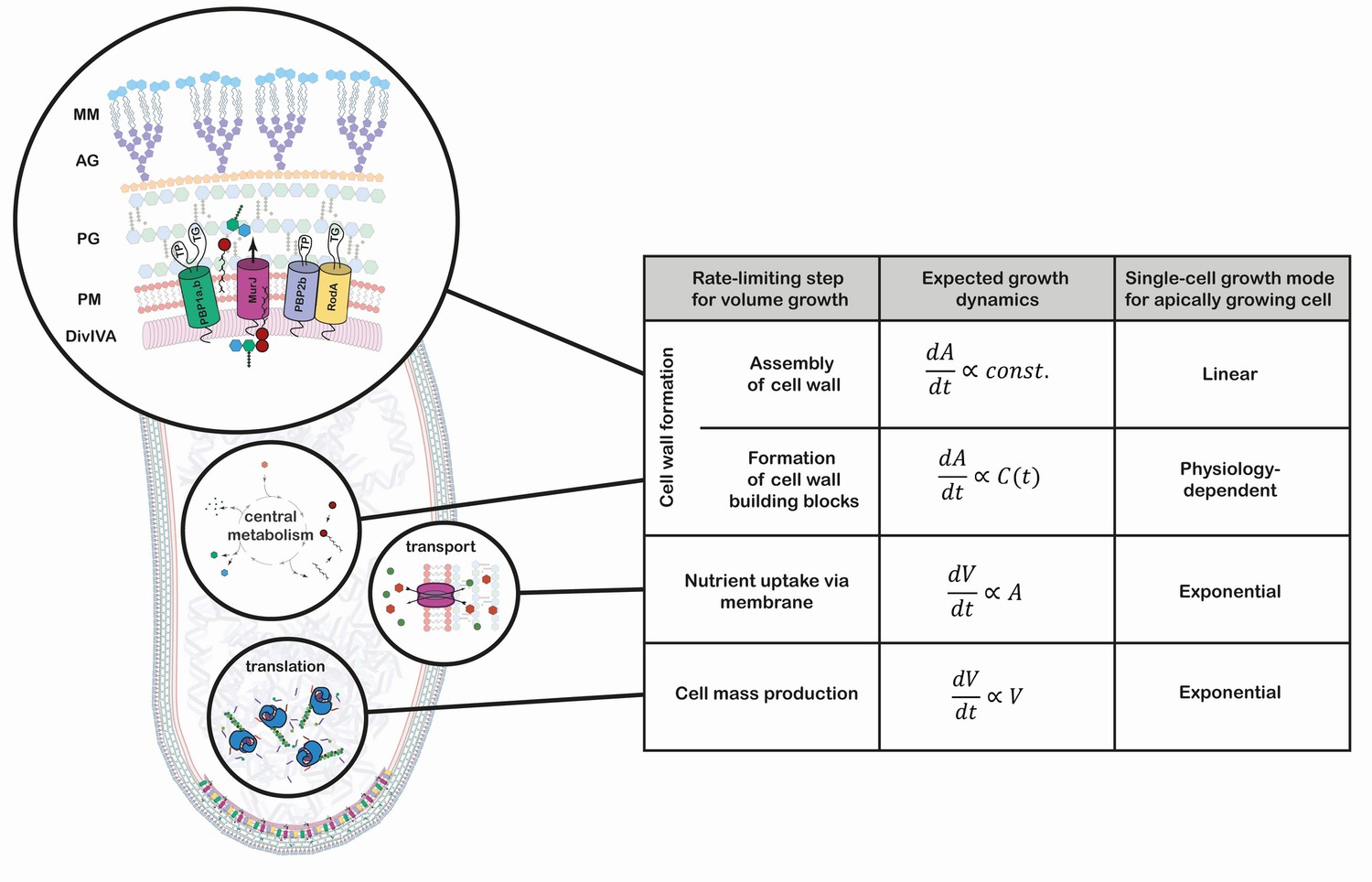
Growth mode analysis for four possible rate-limiting steps for cellular volumegrowth in the apically growing *C. glutamicum*.

Here, $V$ is the cellular volume, $A$ is the cell wall area, and $C (t)$ is the concentration of membrane building blocks in the cytoplasm. A constant cell width is assumed throughout, implying $\frac{d A}{d t} \propto \frac{d V}{d t}$ . A fixed production capacity per unit volume is assumed for the rate-limiting steps 'cell mass production' and 'formation of cell wall building blocks'. For the rate-limiting step 'assembly of cell wall', a constant insertion area at the cell poles is assumed. For an analysis of the single-cell growth mode if cell wall building block formation is the rate-limiting step for growth, see Appendix 1. Cell mass production, specifically ribosome synthesis, has previously been indicated as the rate-limiting step for growth in *E. coli* (Belliveau et al., 2020; Scott et al., 2010; Amir, 2014). Linear growth is observed if the rate-limiting step for volume growth is the cell wall assembly (shown here in a simplified representation). The protein DivIVA serves as a scaffold at the curved membrane of the cell pole for the recruitment of the Lipid-II flippase MurJ and several mono- and bi-functional trans-peptidases (TP) and -gylcosylases (TG). In the process of elongation, peptidoglycan (PG) precursors are integrated into the existing PG sacculus, which serves as a scaffold of the synthesis of the arabinogalactan-layer (AG) and the mycolic-acid bilayer (MM).

Figure 2

Download asset Open asset

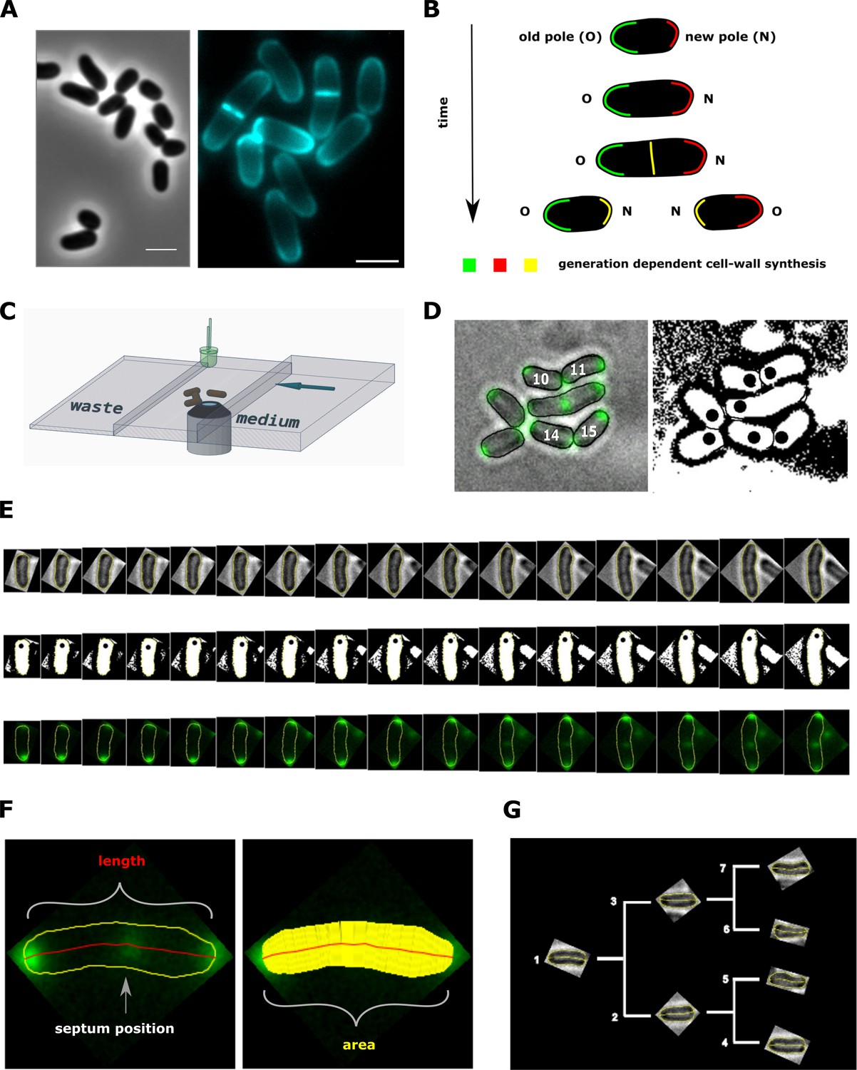
Experimental procedure and image analysis.

(A, left) Phase contrast image of *C. glutamicum* in logarithmic growth phase, indicating the variable size of daughter cells. (A, right) HADA labeling of nascent peptidoglycan (PG), indicating the asymmetric apical growth where the old cell-pole always shows a larger area covered compared to the new pole. The labeling also reveals the variable septum positioning; Scale bar: 2 µm (B) Schematic showing the generation-dependent sites of PG synthesis in *C. glutamicum*, including the maturation of a new to an old cell-pole. (C) Illustration of the microfluidic device for microscopic monitoring of a growing colony. (D) Example screen-shot of the developed method to extract individual cell cycles from a multi-channel time-lapse micrograph. The left panel shows a merging of the bright-field channel and the mCherry-tagged DivIVA together with an individual ID# that is assigned to cells right after division. The black dots in the right panel indicate the new cell pole. (E) Example of an extracted individual cell cycle from birth (left) until prior to division (right), showing the bright-field (top), the orientation (middle) and the localization of mCherry-tagged DivIVA (bottom). (F) Example of the developed single cell analysis algorithm, measuring the length according to the cell’s geometry, as well as the cell’s area and the septum position relative to the new pole. (G) Dendrogram providing the rationale for identification of single cells in a growing colony.

Figure 3

Download asset Open asset

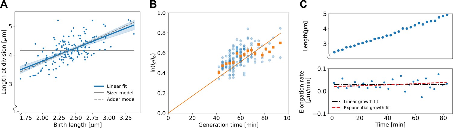
Population-level and single-cell level growth analysis.

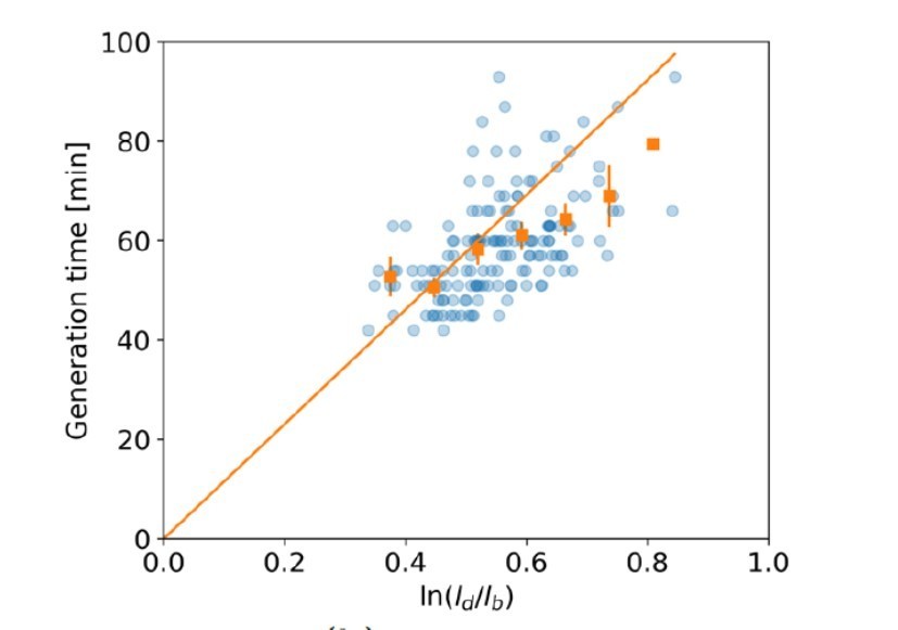
(A) Birth length $l_{b}$ plotted against division length $l_{d}$ for all measured cells, together with a linear fit (blue line), which has a slope of 0.91±0.16. Gray solid line: best fit assuming a pure sizer (slope 0). Gray dashed line: best fit assuming a pure adder (slope 1). The 95% confidence intervals of the linear fit, obtained via bootstrapping, are indicated by the blue shaded region. (B) Generation time versus $l n (\frac{l_{d}}{l_{b}})$ for all cells (blue dots) and the average per generation time (orange squares), with the standard error of the mean shown for all generation times for which at least three data points are available. The orange line represents a linear fit through the generation time averages that passes through the origin. For exponential growth, the averages would lie along this line, and the slope would be equal to the exponential growth rate. (C) Growth trajectory for a single cell (upper panel), together with its derivative for each measurement interval (lower panel). Fits to the derivative are shown for linear growth (black dash-dotted line) and exponential growth (red dashed line).

Figure 4

Download asset Open asset

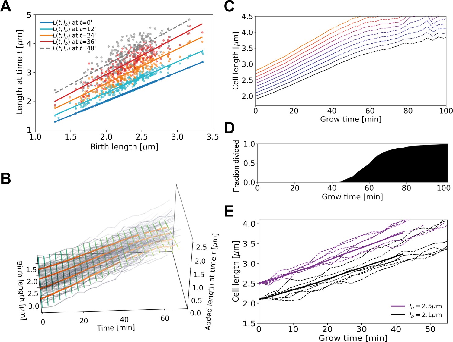
Average elongation curve inference procedure.

(A) For each cell, the length $L (t)$ at different times t since birth is plotted as a function of birth length $l_{b}$ . A linear fit of the resulting ‘wave front’ is performed for each time $t$ . This allows us to determine average cell length $L (t, l_{b})$ at time $t$ as a function of birth length $l_{b}$ . (B) 3D representation of the inference method of average length trajectories, with the added length $L (t, l_{b}) - l_{b}$ on the z-axis. Elongation trajectories for individual cells are indicated in gray, linear fits through all cell lengths at each timestamp are indicated by green lines. The orange lines represent four sample average length trajectories, obtained by connecting all values of the green lines associated with one birth length. Dotted lines represent regimes where averages are biased due to dividing cells. (C) Average elongation trajectories obtained from the fits shown in (A) for a range of birth lengths, starting at 1.9 μm with steps of 0.1 μm (solid lines). The dashed lines represent regions where the inferred elongation curves are biased due to dividing cells, and are excluded from subsequent analysis. (D) Cumulative fraction of cells divided as a function of grow time. (E) Elongation trajectories for cells with birth lengths close to 2.5 μm (purple dashed lines) and birth lengths close to 2.1 μm (black dashed lines) together with their respective inferred average trajectories (purple solid line and black solid line).

Figure 5

Download asset Open asset

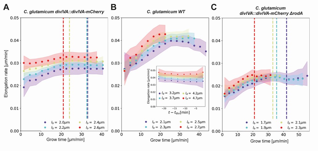
Inferred average elongation rates.

(A) Average elongation rates for four birth lengths (dots), for the DivIVA-labeled cells. The 2σ confidence intervals obtained by bootstrapping are indicated by the shaded areas. Vertical dashed lines: average onset of septum formation per birth length. (B) Average elongation rate trajectories for the wild-type cells, confidence intervals shown as in (A). Inset: average elongation trajectories as a function of the time until division. (C) Average elongation rate trajectories for the *ΔrodA* mutant, confidence intervals shown as in (A).

Figure 6

Download asset Open asset

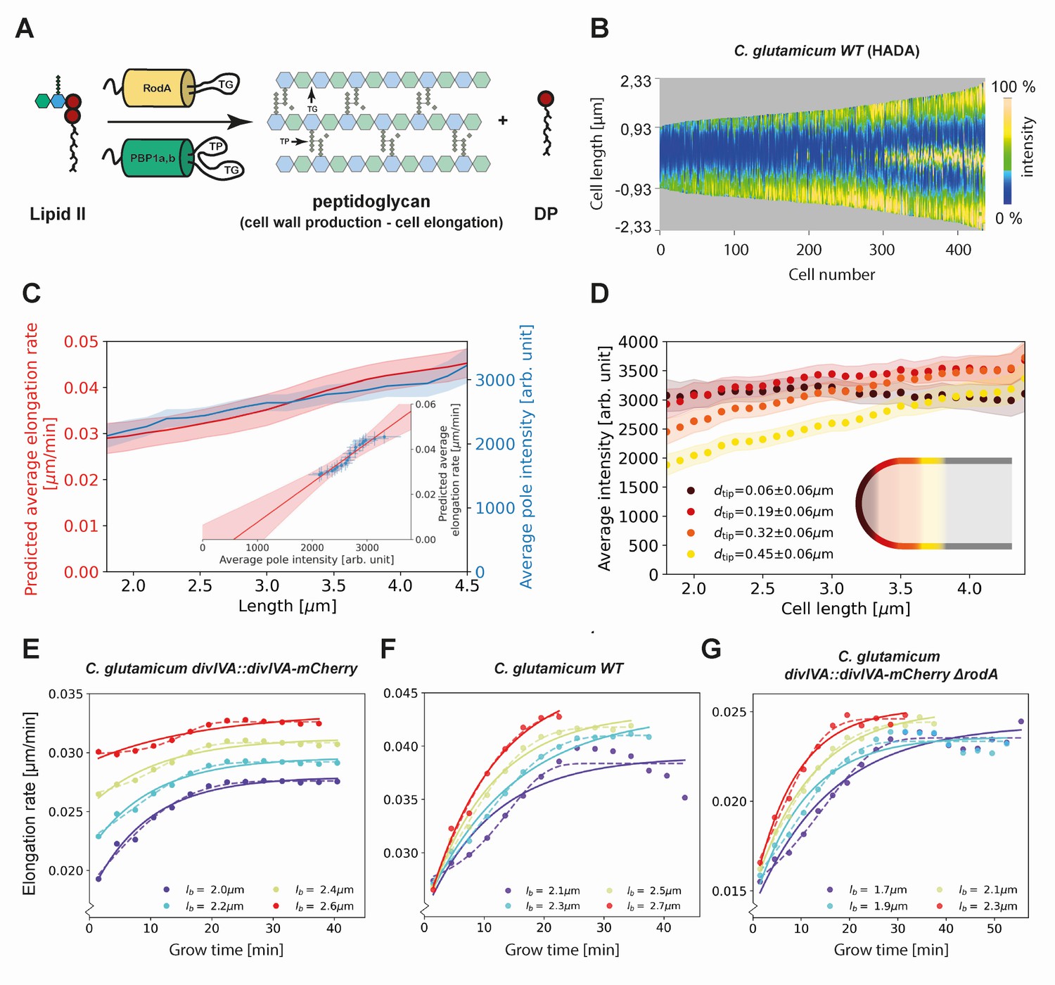
Modeling of average elongation rates using HADA staining results.

(A) Schematic depicting cell wall formation via Lipid-II and transgrlycosylases (TG's). The corresponding Michaelis-Menten equation describes the change of length over time as function of the Lipid-II concentration $C (t)$ and the number of the TG sites $N (t)$ . (B) Demograph of *C. glutamicum* cells stained with HADA. Cell are ordered by length, with the stronger signal oriented downwards. (C) Average elongation rate as a function of cell length (red), predicted from obtained average elongation rate curves (Appendix 8), together with the average HADA staining intensity at the cell pole after background correction (blue). The cell pole is defined here as the region within 0.77 µm (60 pixels) of the cell tip. The shaded regions indicate the 2XSEM bounds. For both curves, a moving average over cells within 0.7 µm of each x-coordinate is applied over the underlying data. Inset: predicted average elongation rate versus average HADA staining intensity (blue dots). A linear fit through the result (red line) is consistent with a proportional relationship. (D) Average HADA intensity as a function of cell length, shown for four regions close to the cell tip. A moving average over cells within 0.7 µm of each x-coordinate is applied over the underlying data. (**E-G**) Dots: average elongation rate curves as shown in Figure 5A. Solid lines: best fit of elongation model from Equation (2), which assumes constant transglycosylase recruitment. Dashed lines: best fit of elongation model from Equation (3), which assumes an exponential increase of transglycosylase recruitment.

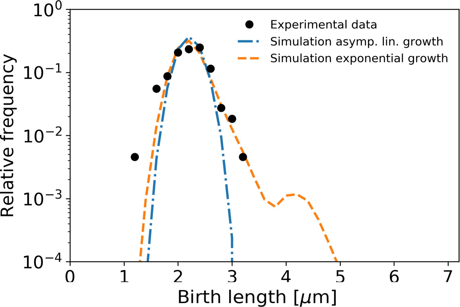
Figure 7

Download asset Open asset

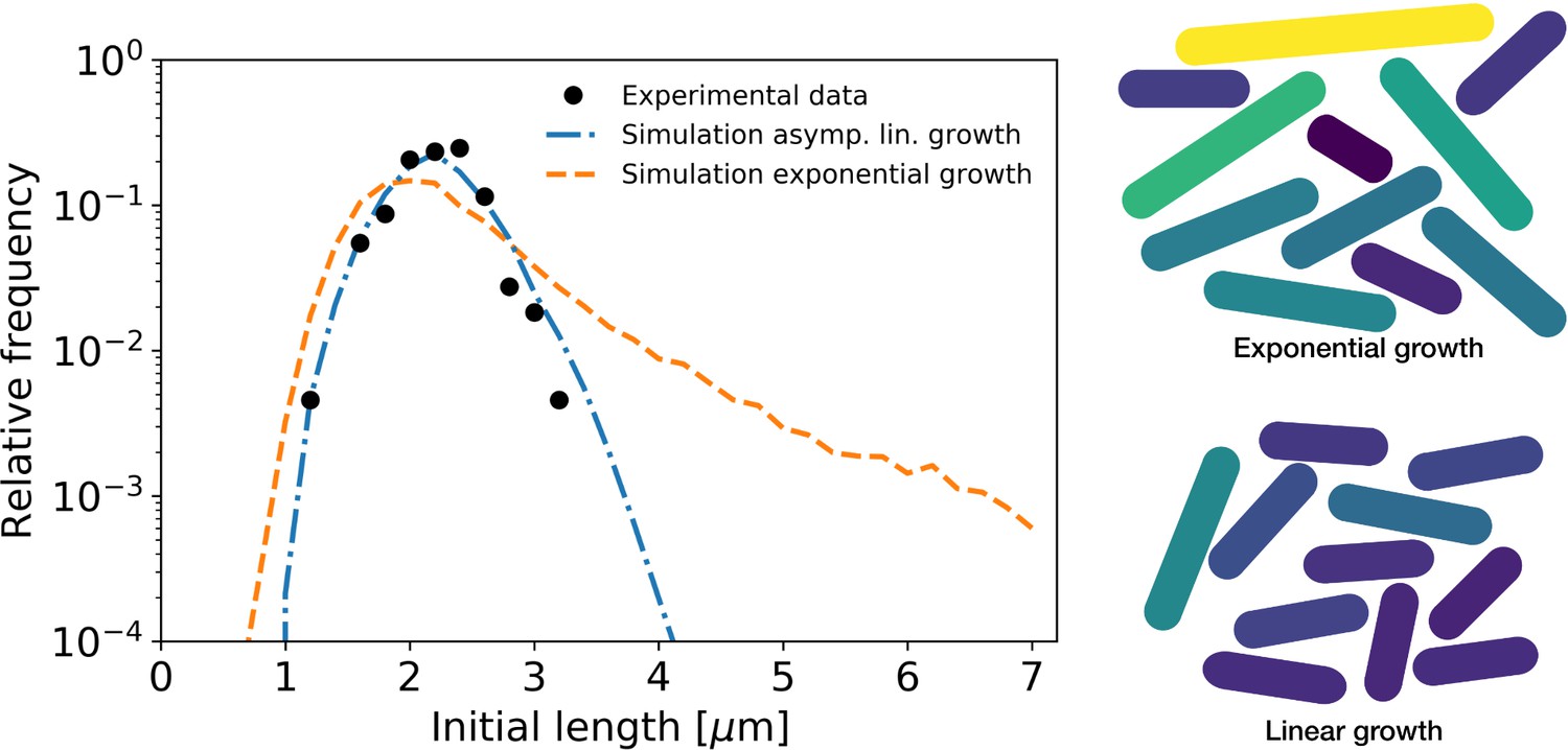
Simulation of population growth for asymptotically linear and exponential growth.

Left: birth length distribution for simulated asymptotically linear growth (blue dash-dotted line), and for simulated exponential growth (orange dashed line). For both simulations, all relevant growth parameters and distributions are obtained directly from the experimental data. Black dots: experimental birth length distribution. Right: sample of 11 cells from the exponential and asymptotically linear growth simulations, color coded according to length.

Appendix 1—figure 1

Download asset Open asset

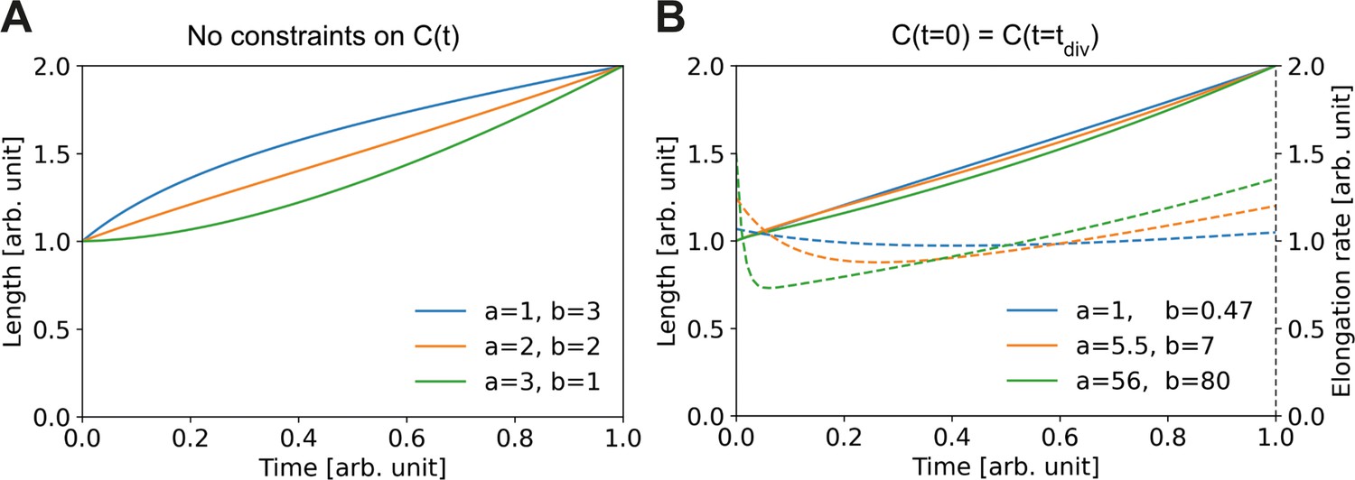
Elongation curves assuming building block availability is the limiting step for growth.

(A) Numerically obtained solutions for $V (t)$ , from the set of coupled differential equations Equation (A2) and Equation (A3). For all solutions, $V (0) = 1$ and $V (1) = 2$ are imposed. (B) Solutions as in (A), but with the additional constraint that the concentrations before and after division are the same, i.e. $C (t = 0) = C (t = t_{div})$ . Solid lines: solutions for $V (t) .$ Dashed lines: corresponding $\frac{d V (t)}{d t}$ , which are proportional to the concentration $C (t)$ per Equation (A3).

Appendix 2—figure 1

Download asset Open asset

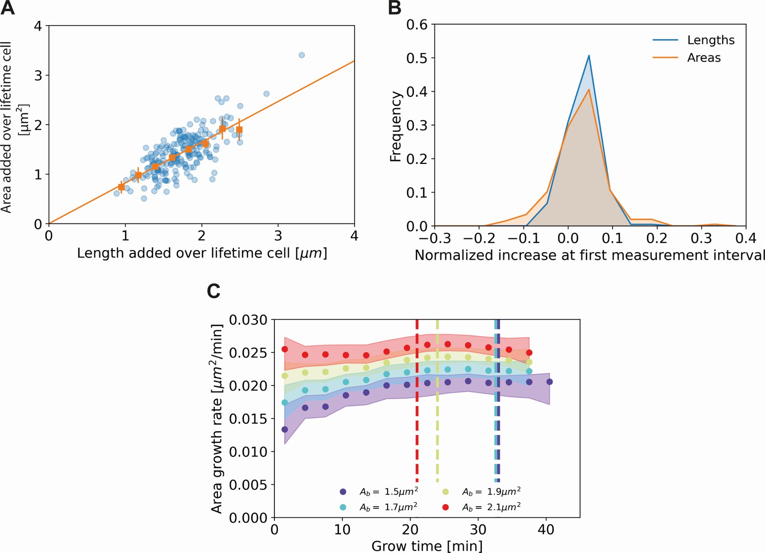
Comparing cell length and cell area measurements.

(A) Length added versus area added over the cell lifetime for all cells included in our analysis (blue dots), together with averaged values at 0.2 μm intervals (orange squares) and 95% confidence intervals (orange vertical lines). The results are consistent with a proportional relationship (orange line). (B) Histogram of the normalized increase at first measurement interval using cell lengths (blue) and areas (orange). For the cellular lengths, this quantity is defined as $\frac{L (t = 3 m i n) - L (t = 0)}{⟨ l_{b} ⟩}$ , whereas for the areas it is defined as $\frac{A (t = 3 m i n) - A (t = 0)}{⟨ A_{b} ⟩}$ , with $A (t)$ the area at time $t$ and $A_{b}$ the birth area. The wider distribution for the areas suggests a higher measurement noise for this quantity. (C) Area growth rate for DivIVA-labeled cells using estimated cell areas. The trajectories are consistent with those obtained from cell lengths (Main Text Figure 5A).

Appendix 2—figure 2

Download asset Open asset

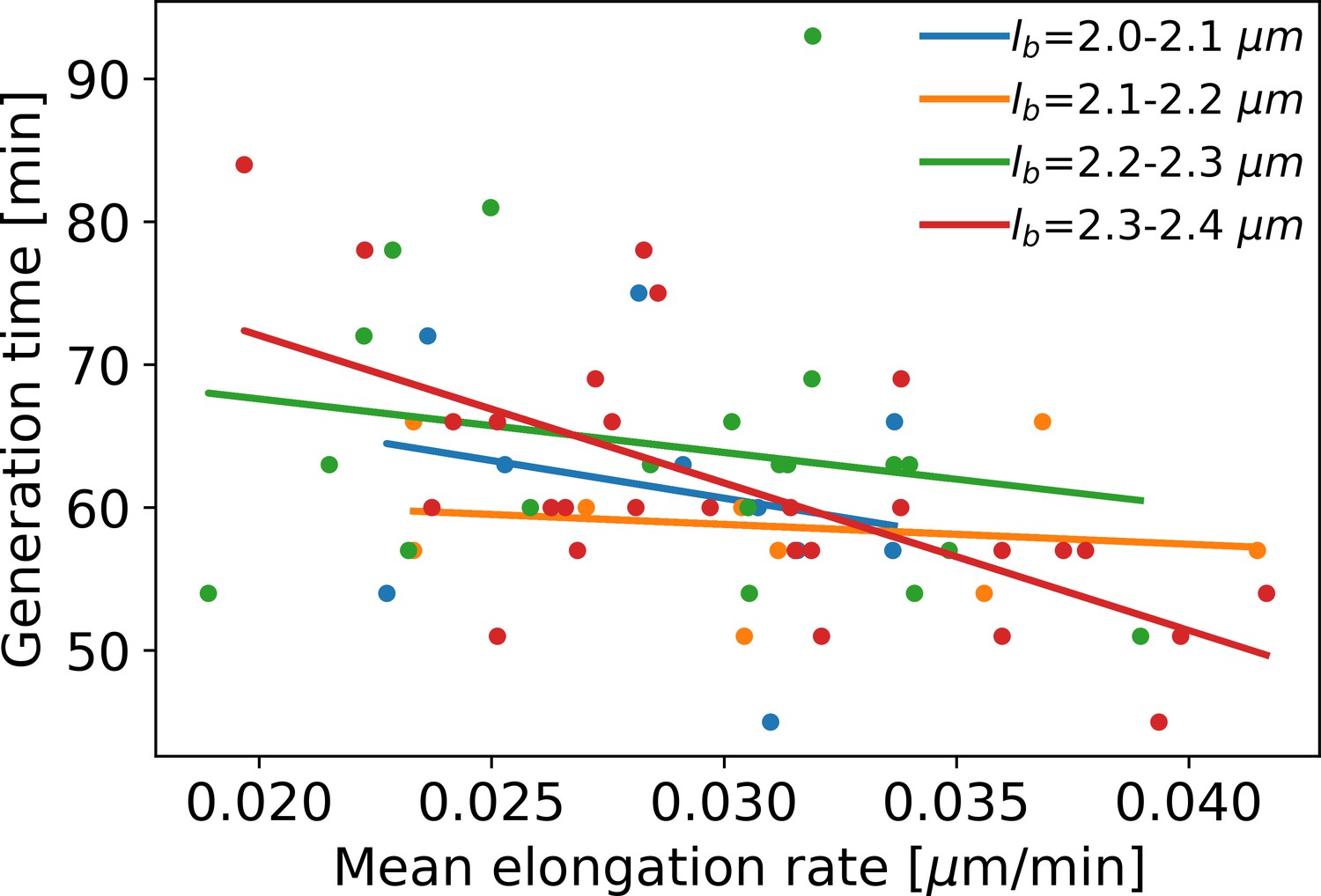
Mean elongation rate versus generation time for cells in four different birth size bins.

Linear fits are indicated by solid lines. As generation times within a birth size bin tend to be shorter for faster-growing cells, the elongation rate curves obtained with our method become biased after the first division event. This justifies only using the part of the elongation rate curves until the first division event for further analysis.

Appendix 2—figure 3

Download asset Open asset

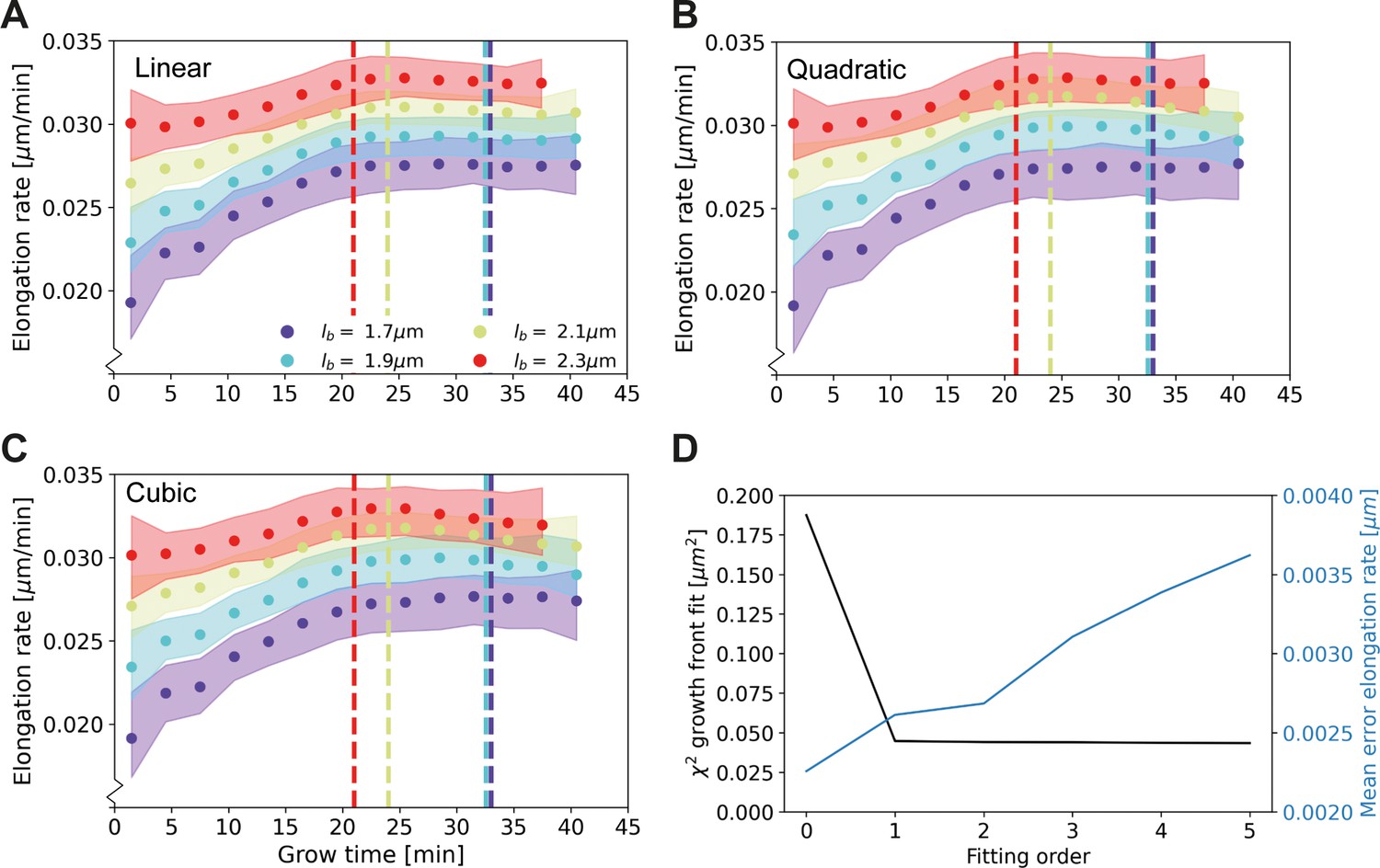
Elongation rate curves for different orders of the wave front fit of Main Text Figure 3A: Linear (A), quadratic (B), and cubic (C).

(D) χ² of the fit of the wave front of Main Text Figure 3A for different fitting orders, together with the mean error on the elongation rate curves. The negligible improvement of the goodness-of-fit after the first order justifies the use of a linear fit for further analysis.

Appendix 2—figure 4

Download asset Open asset

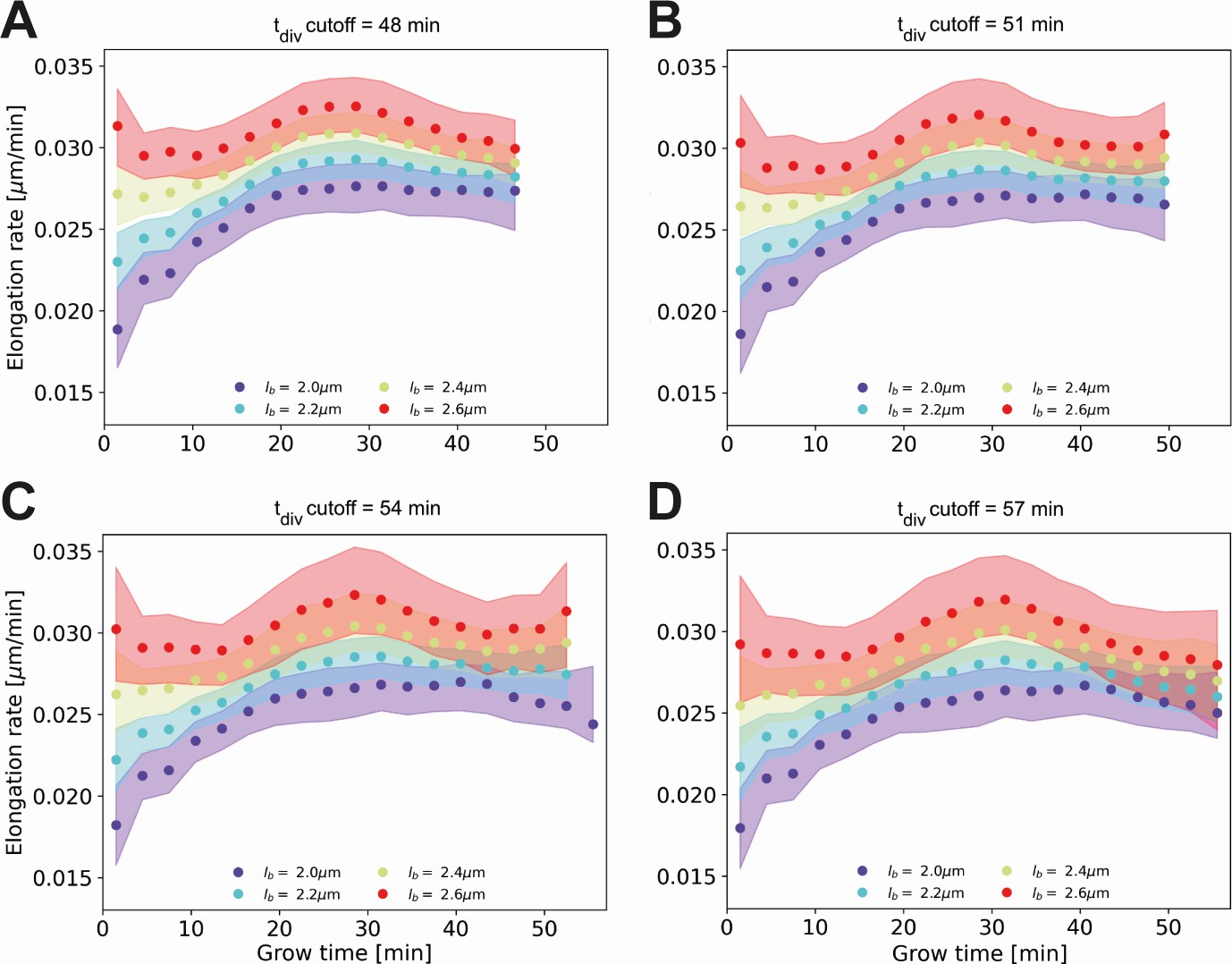
Conditional elongation rate curves, conditioned on DivVIA-labeled cells that have a generation time larger than a set cutoff value: 48 min (A), 51 min (B), 54 min (C) and 57 min (D).

The inferred elongation rate curves still display similar growth behavior to the unconditioned population (Main Text Figure 5A), but exhibit an overall downwards shift with increasing cutoff times. For larger cutoff times, the number of cells included decreases, resulting in larger errors on the inferred elongation rates. The linear growth phase observed until the cutoff time for the unconditioned population is seen to persist for longer grow times.

Appendix 2—figure 5

Download asset Open asset

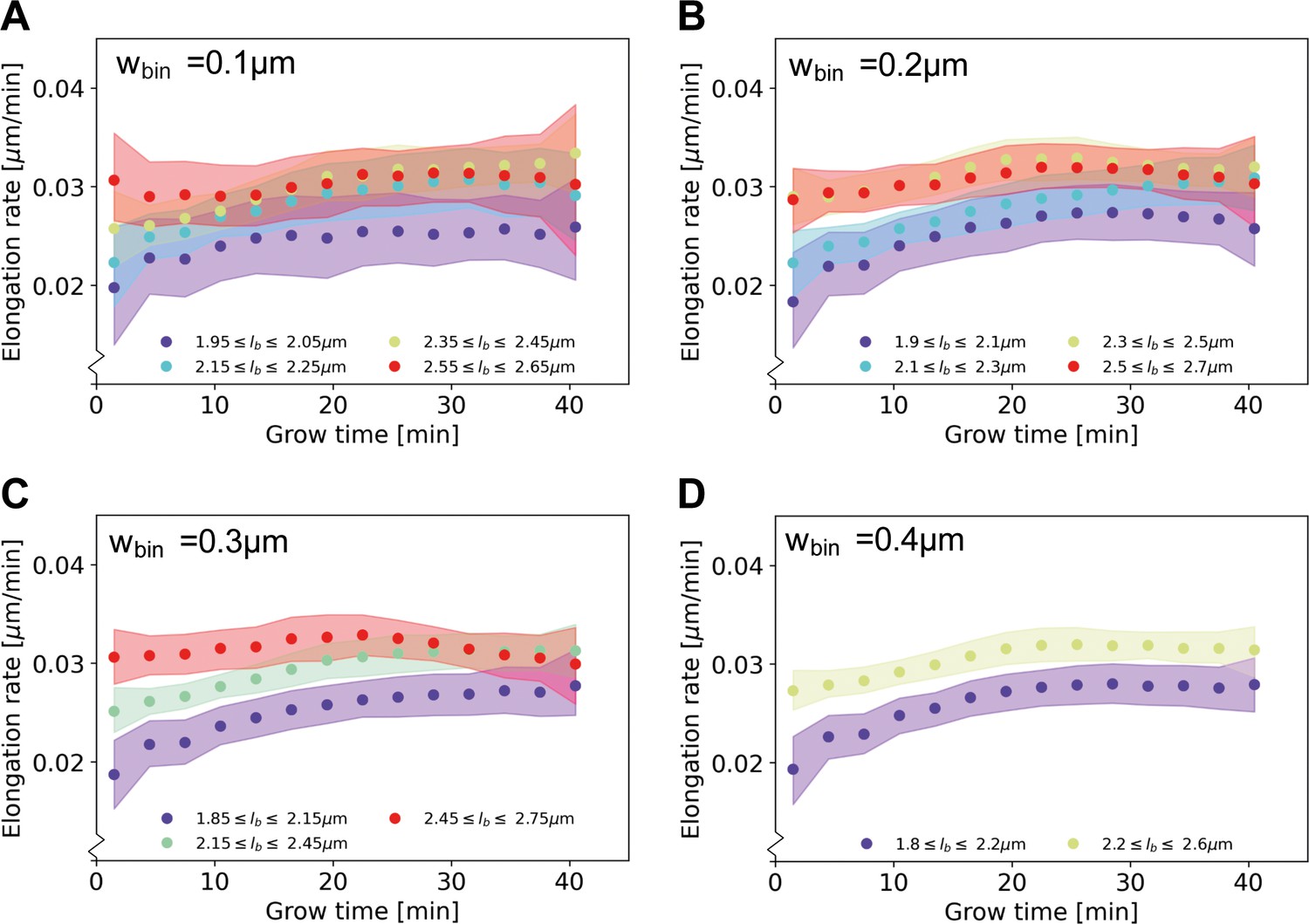
Elongation rate curves obtained through a binning procedure.

Cells are divided into birth length bins, and for each bin the average length as a function of grow time is calculated. The resulting elongation curves are smoothened according to the same procedure as the elongation curves presented in the main text (see Appendix 5). From the smoothened elongation curves, elongation rates are calculated as a function of grow time. Results are shown for a bin width of 0.1 μm (A), 0.2 μm (B), 0.3 μm (C), 0.4 μm (D), where each $l_{b}$ indicates the center of the birth length bin.

Appendix 2—figure 6

Download asset Open asset

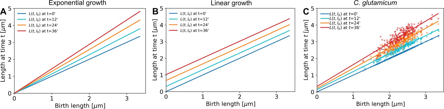
A linear fit through the cell lengths at each time step would be enough to describe exponential growth (A, offset is zero for all time stamps) as well as linear growth (B, slope is equal to 1 for all time stamps).

*C. glutamicum* (C) matches neither of these growth modes.

Appendix 2—figure 7

Download asset Open asset

The average DivIVA-mCherry signal from the cell center over time is shown for DivIVA-labeled cells (A) and *ΔrodA* DivIVA-labeled cells (B).

The cell center is here defined as the region between 20% and 80% of the total cell length. The onsets of septum formation, derived from the DivIVA signal-mCherry signal, are indicated by the dashed lines; these do not consistently coincide with the levelling off of elongation rates (Main Text Figure 5A). This is inconsistent with the leveling off being due to a competition between polar growth and septum formation.

Appendix 2—figure 8

Download asset Open asset

Calculation of corrected polar HADA intensity, illustrated for two HADA profiles.

Solid line: HADA intensity profile. Dashed horizontal line: minimum of HADA profile. Dashed vertical lines: boundary of polar region. Shaded area: calculated total polar intensity. Results shown for a cell with a length of 2.3 μm (A) and 4.4 μm (B).

Appendix 2—figure 9

Download asset Open asset

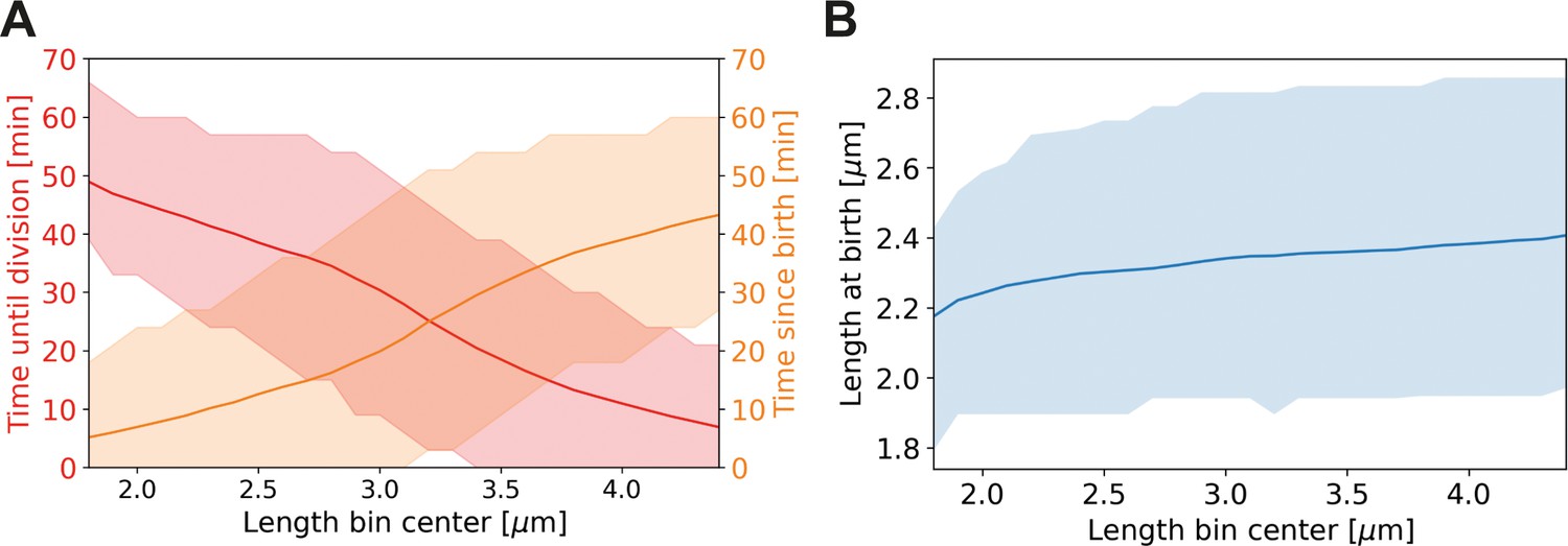
Average properties of wild-type cells as a function of length.

Values are shown over the range of observed lengths in the HADA staining experiment, using a moving average with the same width (±0.7 µm) as in Main Text Figure 6C. (A) Red line: average time until division, together with the two standard deviation bounds (red shaded area). Orange line: average time since birth, together with two standard deviation bounds (orange shaded area). (B) Blue line: average birth length for each birth length bin (blue line), together with the two standard deviation bounds (blue shaded area).

Appendix 2—figure 10

Download asset Open asset

Proportionality between average pole intensity and predicted average elongation rate for different polar region definitions.

Average elongation rate as a function of cell length (red), predicted from obtained average elongation rate curves, together with the average HADA staining intensity at the cell pole after background correction (blue). Results are shown for a polar region defined to be within 0.51 µm (A) and 1.0 µm (B) of the cell tip.

Appendix 2—figure 11

Download asset Open asset

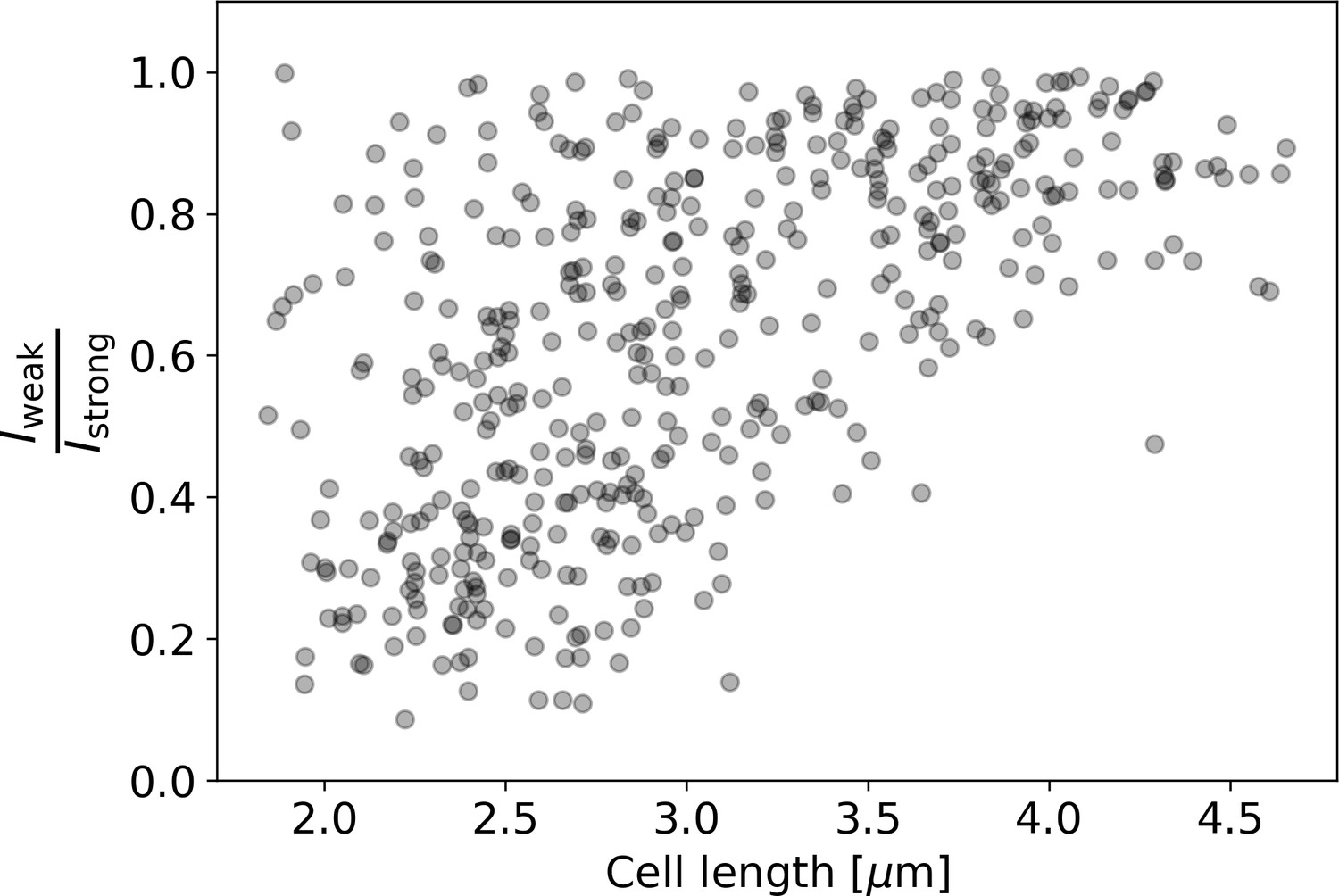
Ratio of intensities between the weaker and the stronger pole of each cell in the HADA staining experiment.

Polar intensities are calculated as described in Appendix 2—figure 8. Here, $I_{weak}$ denotes the intensity of the cell pole with the weaker HADA intensity signal, and $I_{strong}$ denotes the intensity of the pole with the stronger signal. For NETO-like growth (Hannebelle et al., 2020), a clustering of values around 0 (before new end take off) and 1 (after new end take off) would be expected, which is not observed here.

Appendix 3—figure 1

Download asset Open asset

Estimation of measurement noise procedure.

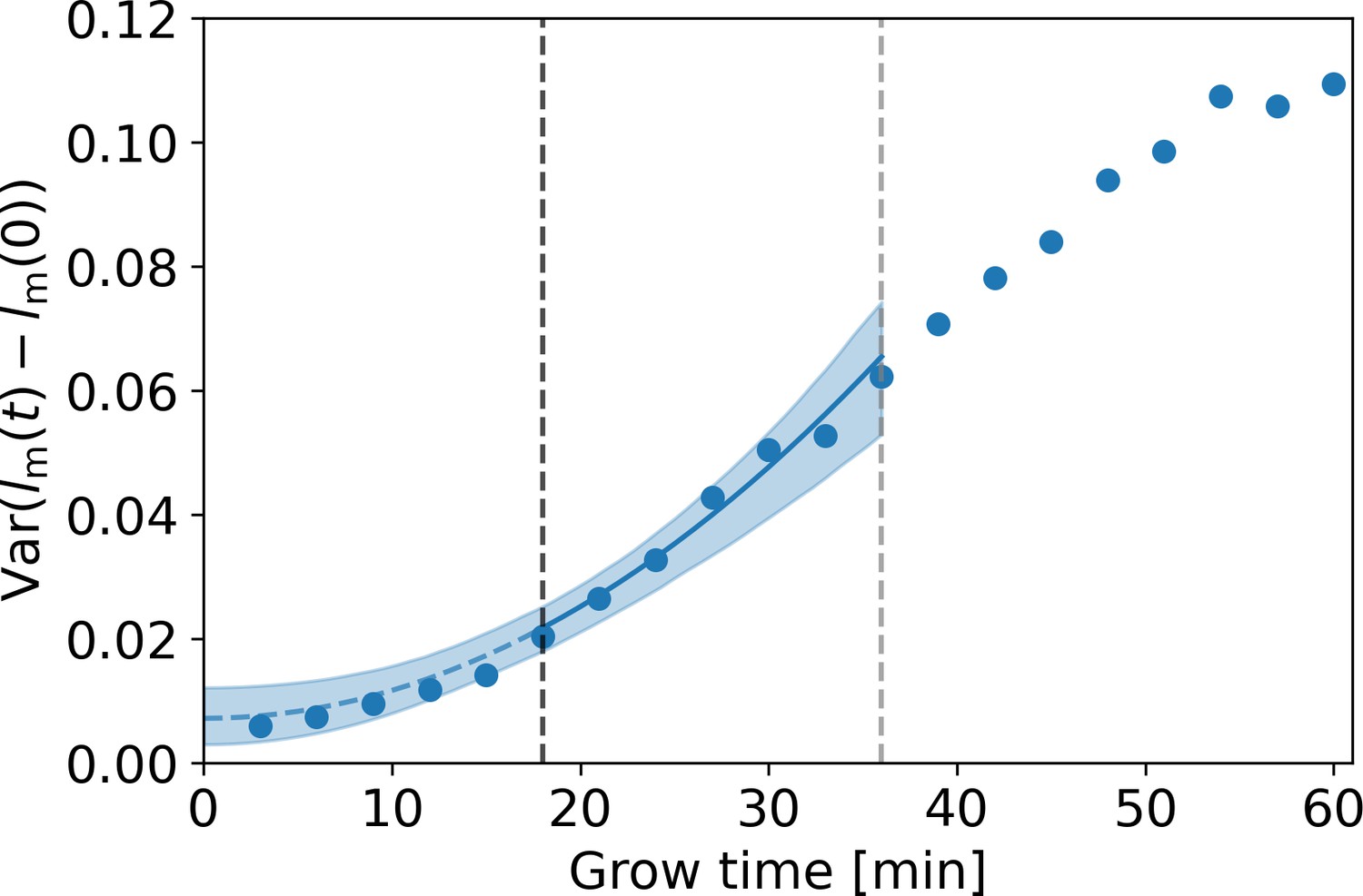
Blue dots: variance of $l_{m} (t) - l_{m} (0)$ as a function of grow time for the DivIVA-labeled cells, with $l_{m} (t)$ the measured cellular length at grow time $t$ . A fit of Equation (A7) under substitution of Equation (A9) (blue line) is made to the points between the onset of linear growth (black dashed line) and the moment of first division (gray dashed line). The value of the extrapolated fit (blue dashed line) at t=0 is equal to $2 σ_{n}^{2}$ , with $σ_{n}$ the standard deviation of the measurement noise. The 95% confidence intervals of the model fit (blue shaded area) are obtained via bootstrapping.

Appendix 4—figure 1

Download asset Open asset

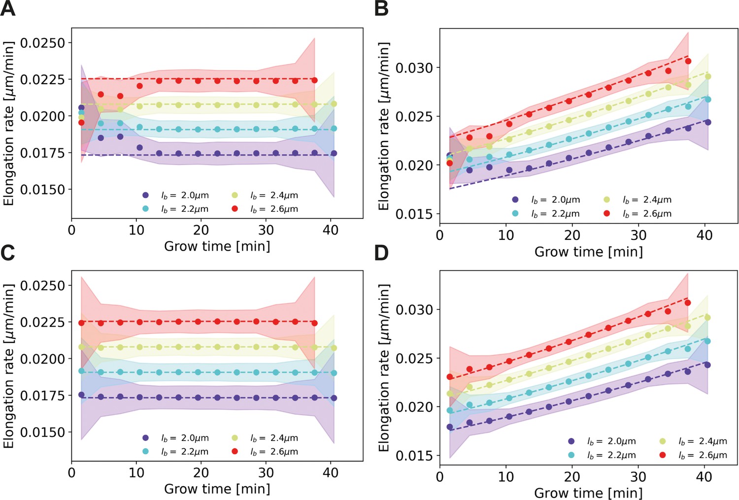
Elongation rate inference on simulated data sets, with and without bias correction procedure for assigned birth lengths.

For all panels: dashed lines: input elongation rates. Dots: mean inferred average elongation rates, obtained by applying our inference procedure to 1000 simulated data sets. Shaded areas: 2σ bounds on the inferred elongation rates. For all simulated data sets, the measurement noise is drawn from a Gaussian distribution with a standard deviation of 0.075 μm, matching the estimated experimental noise (Appendix 4). The population size and birth length distribution are chosen to match those observed for the DivIVA-labeled cells. Simulation conditions: (A) Linear input elongation rates constructed by setting $l (t) = l_{b} + 0.26 l_{b} t$ . No bias correction procedure for assigned birth lengths is applied. (B) Exponential input elongation rates constructed by setting $l (t) = l_{b} e^{0.26 t} .$ No bias correction procedure for assigned birth lengths is applied. (C) Input elongation rates as in (A). The bias correction procedure for assigned birth lengths is applied. (D) Input elongation rates as in (B). The bias correction procedure for assigned birth lengths is applied.

Appendix 5—figure 1

Download asset Open asset

Average elongation rate curves obtained after Gaussian smoothing of the inferred average elongation curves (dots), together with average elongation rate curves obtained from unsmoothed average elongation curves (dashed lines).

Appendix 6—figure 1

Download asset Open asset

Inferred elongation rates as a function of the time until division, shown for DivIVA-labeled cells (A), wild-type cells (B) and the *ΔrodA* mutant (C).

To obtain these curves, the elongation rate inference procedure described in the Main Text was applied, with the modification that $L (t - t_{div}, l_{d})$ was calculated, rather than $L (t, l_{b})$ . This yields average elongation rate curves as a function of division length, which are unbiased until the growth time of the shortest-lived cell (left endpoints of the elongation rate curves). The inferred linear growth regime for later grow times persists until division.

Appendix 7—figure 1

Download asset Open asset

Recovery of inferred elongation rates from simulated growth Dashed lines: input elongation rates, as inferred for DivIVA-labeled cells (Main Text Figure 5A).

Dots: average of elongation rates inferred from simulated growth experiment. Shaded areas: 95% confidence intervals inferred from simulated growth experiment, obtained via bootstrapping.

Appendix 10—figure 1

Download asset Open asset

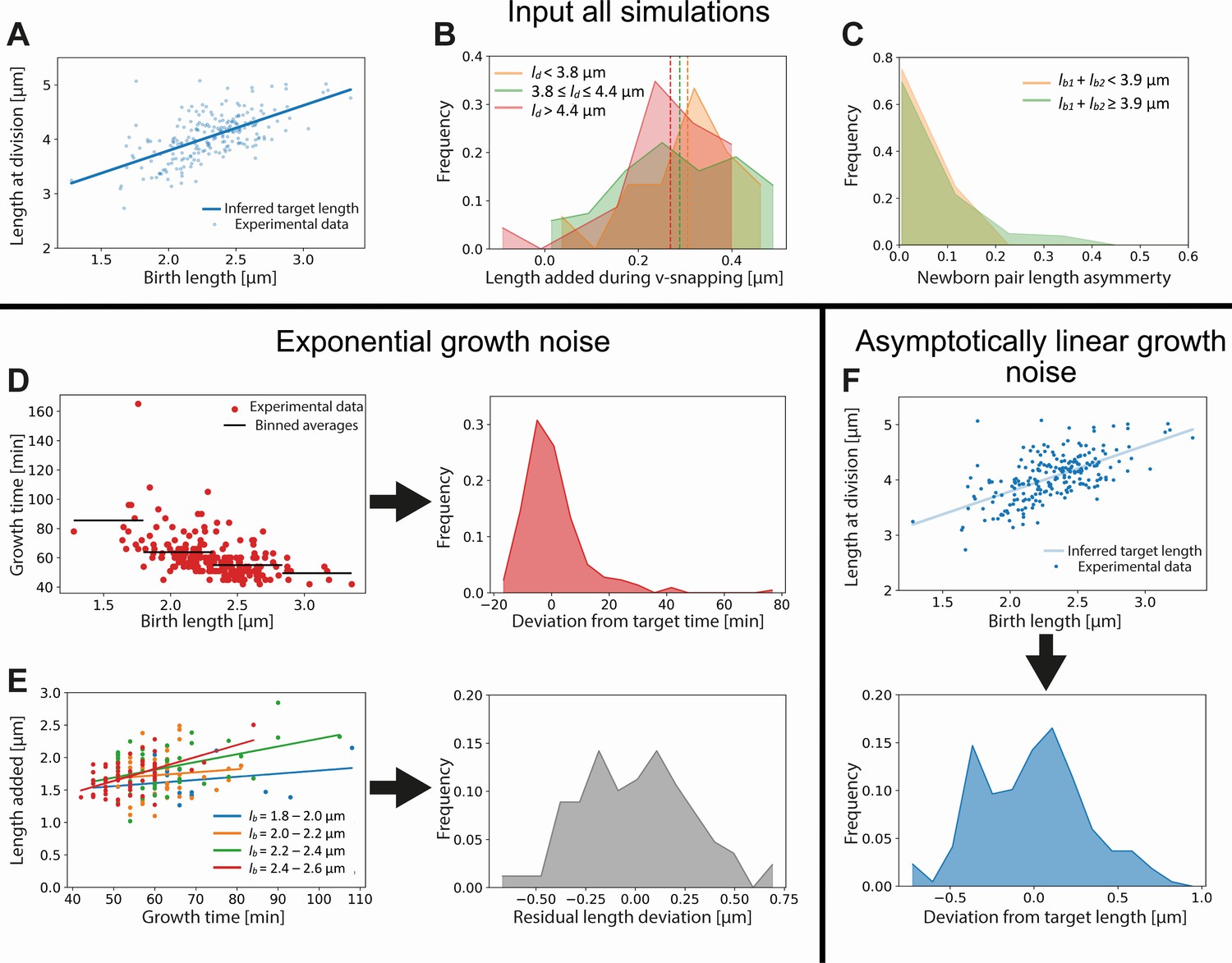
Input used for simulations of exponential and asymptotically linear growth.

For both simulations, a linear fit of the division length versus birth length is used to define a target length (A). The length added during the V-snap at division is randomly drawn from the distribution corresponding to the division length of the simulated cell (B). The experimental data is divided into three subpopulations according to division length (red, green, and orange distributions), as the average length added during V-snap decreases with division length (dashed lines). The asymmetry of the daughter cells is randomly drawn from the distribution corresponding to the combined length of the simulated daughters (C). As the asymmetry is lower for the smallest daughter cells, the experimental data is divided into two subpopulations (red and green distributions). For the simulation of exponential growth, two noise sources are needed as input. The time-additive noise is randomly drawn from the distribution of deviations from target growth times (D). This distribution is obtained from the deviations of single-cell growth times from the average of their birth length bin. All growth variability not captured by growth time variations is calculated for four narrow birth length bins (blue, orange, green, and red points) (E). From the distribution of deviations of added lengths from a linear fit for each initial size bin, a size-additive noise term is randomly drawn. For the linear growth simulation, only a single additive noise term is required, which is randomly drawn from the distribution of deviations of cells lengths at division from the target division length (F).

Appendix 10—figure 2

Download asset Open asset

Birth length distributions as in Main Text Figure 7, but with single-cell variability in division symmetry, growth time, and (residual) length deviation reduced by a factor 3.

The second peak in the length distribution of exponential growth is attributed to the large time deviation of one single cell seen in Appendix 10—figure 1D.

Author response image 1

Download asset Open asset

$\ln (\frac{l_{d}}{l_{b}})$ versus generation time for all cells (blue dots) and the average per generation time bin (orange squares), with the standard error of the mean shown for all generation times for which at least 3 data points are available.

Author response image 2

Download asset Open asset

$\ln (\frac{l_{d}}{l_{b}})$ versus generation time for three simulated datasets (blue dots), and the average per generation time (orange squares), with the standard error of the mean.

The orange line represents a linear fit through the generation time averages that passes through the origin. For each simulation, birth length and division length pairs were sampled from the DivIVA-labelled cell dataset. The number of such pairs is equal to the number of cells in the data set. Each simulated cell started at an assigned birth length, and was grown until the minimum difference with the corresponding division length was reached. The inferred measurement noise (Appendix 3) was applied to all simulated data points. (A) Exponential growth, constructed by setting $l (t) = l_{b} e^{0.26 t}$ . (B) Linear growth, constructed by setting 𝑙(𝑡) = 𝑙_b + 2.08𝑡. (C) A mixed model, where cells grow exponentially for the first 30 minutes, and switch to linear growth from then on.

Tables

Key resources table

Reagent type (species) or resource	Designation	Source or reference	Identifiers	Additional information
Gene (include species here)	‘divIVA’; ‘rodA’	KEGG	‘cg2361’; ‘cg0061’
Strain, strain background (Corynebacterium glutamicum)	‘ATCC 13032’; ‘RES 167’	‘ATCC’; ‘Tauch et al., 2002’	‘13032’;”RES 167’
Genetic reagent (Corynebacterium glutamicum)	‘RES 167 divIVA::divIVA-mCherry’;”RES 167 ∆ rodA, divIVA::divIVA-mCherry’	‘Donovan et al., 2012'; ‘Sieger et al., 2013’	‘CDC010’; ‘BSC002’
Chemical compound, drug	HADA stain	Tocris Bioscience	6647/5
Software, algorithm	MorpholyzerGT	This paper		see Materials and methods
Other	CellASIC microfluidic System	Millipore	B04A

Appendix 9—table 1

Parameter values obtained by fitting Main Text Equation (2) to inferred elongation rate curves.

The values shown in column 4 and 6 are an average over the four birth lengths of each condition.

Genotype	$l_{b}$ [μm]	$β$ [ $t^{- 1}$ ]	$⟨ β ⟩$ [ $t^{- 1}$ ]	$\frac{N (t = 0)}{N^{max}}$	$⟨ \frac{N (t = 0)}{N^{max}} ⟩$
wild-type	2.1	0.088	0.085	0.67	0.62
	2.3	0.068		0.62
	2.5	0.093		0.62
	2.7	0.089		0.58
divIVA::divIVA-mCherry	2.0	0.109	0.088	0.69	0.80
	2.2	0.100		0.77
	2.4	0.087		0.84
	2.6	0.054		0.88
divIVA::divIVA-mCherry ΔrodA	1.7	0.063	0.087	0.61	0.64
	1.9	0.094		0.65
	2.1	0.084		0.64
	2.3	0.11		0.65

Appendix 9—table 2

Parameter values obtained by fitting Main Text Equation (3) to inferred elongation rate curves.

The values shown in columns 5 and 7 are an average over the four birth lengths of each condition.

Genotype	$l_{b}$ [μm]	$β$ [ $t^{- 1}$ ]	$γ$ [ $t^{- 1}$ ]	$< β e^{γ t} >_{t < 20 m i n}$ [ $t^{- 1}$ ]	$\frac{N (t = 0)}{N^{max}}$	$⟨ \frac{N (t = 0)}{N^{max}} ⟩$
wild-type	2.1	0.016	0.162	0.13	0.72	0.67
	2.3	0.039	0.086		0.67
	2.5	0.058	0.080		0.65
	2.7	0.082	0.050		0.62
divIVA::divIVA-mCherry	2.0	0.072	0.06	0.14	0.71	0.82
	2.2	0.050	0.09		0.79
	2.4	0.025	0.14		0.86
	2.6	0.005	0.25		0.92
divIVA::divIVA-mCherry ΔrodA	1.7	0.023	0.094	0.12	0.67	0.68
	1.9	0.039	0.092		0.69
	2.1	0.064	0.050		0.67
	2.3	0.064	0.100		0.68

Additional files

Source data 1 HADA staining data.: https://cdn.elifesciences.org/articles/70106/elife-70106-data1-v4.zip
Download elife-70106-data1-v4.zip
Source data 2 Elongation measurement data.: https://cdn.elifesciences.org/articles/70106/elife-70106-data2-v4.zip
Download elife-70106-data2-v4.zip
Transparent reporting form: https://cdn.elifesciences.org/articles/70106/elife-70106-transrepform-v4.docx
Download elife-70106-transrepform-v4.docx

Download links

A two-part list of links to download the article, or parts of the article, in various formats.

Downloads (link to download the article as PDF)

Article PDF

Open citations (links to open the citations from this article in various online reference manager services)

Mendeley

Cite this article (links to download the citations from this article in formats compatible with various reference manager tools)

Joris JB Messelink
Fabian Meyer
Marc Bramkamp
Chase P Broedersz

(2021)

Single-cell growth inference of Corynebacterium glutamicum reveals asymptotically linear growth

eLife 10:e70106.

https://doi.org/10.7554/eLife.70106

Share this article

Cite this article

Growth mode analysis for four possible rate-limiting steps for cellular volumegrowth in the apically growing C. glutamicum.

Experimental procedure and image analysis.

Population-level and single-cell level growth analysis.

Average elongation curve inference procedure.

Inferred average elongation rates.

Modeling of average elongation rates using HADA staining results.

Simulation of population growth for asymptotically linear and exponential growth.

Elongation curves assuming building block availability is the limiting step for growth.

Comparing cell length and cell area measurements.

Mean elongation rate versus generation time for cells in four different birth size bins.

Elongation rate curves for different orders of the wave front fit of Main Text Figure 3A: Linear (A), quadratic (B), and cubic (C).

Conditional elongation rate curves, conditioned on DivVIA-labeled cells that have a generation time larger than a set cutoff value: 48 min (A), 51 min (B), 54 min (C) and 57 min (D).

Elongation rate curves obtained through a binning procedure.

A linear fit through the cell lengths at each time step would be enough to describe exponential growth (A, offset is zero for all time stamps) as well as linear growth (B, slope is equal to 1 for all time stamps).

The average DivIVA-mCherry signal from the cell center over time is shown for DivIVA-labeled cells (A) and ΔrodA DivIVA-labeled cells (B).

Calculation of corrected polar HADA intensity, illustrated for two HADA profiles.

Average properties of wild-type cells as a function of length.

Proportionality between average pole intensity and predicted average elongation rate for different polar region definitions.

Ratio of intensities between the weaker and the stronger pole of each cell in the HADA staining experiment.

Estimation of measurement noise procedure.

Elongation rate inference on simulated data sets, with and without bias correction procedure for assigned birth lengths.

Average elongation rate curves obtained after Gaussian smoothing of the inferred average elongation curves (dots), together with average elongation rate curves obtained from unsmoothed average elongation curves (dashed lines).

Inferred elongation rates as a function of the time until division, shown for DivIVA-labeled cells (A), wild-type cells (B) and the ΔrodA mutant (C).

Recovery of inferred elongation rates from simulated growth Dashed lines: input elongation rates, as inferred for DivIVA-labeled cells (Main Text Figure 5A).

Input used for simulations of exponential and asymptotically linear growth.

Birth length distributions as in Main Text Figure 7, but with single-cell variability in division symmetry, growth time, and (residual) length deviation reduced by a factor 3.

ln⁡(ldlb) versus generation time for all cells (blue dots) and the average per generation time bin (orange squares), with the standard error of the mean shown for all generation times for which at least 3 data points are available.

ln⁡(ldlb) versus generation time for three simulated datasets (blue dots), and the average per generation time (orange squares), with the standard error of the mean.

Parameter values obtained by fitting Main Text Equation (2) to inferred elongation rate curves.

Parameter values obtained by fitting Main Text Equation (3) to inferred elongation rate curves.

Source data 1

Source data 2

Transparent reporting form

Downloads (link to download the article as PDF)

Open citations (links to open the citations from this article in various online reference manager services)

Cite this article (links to download the citations from this article in formats compatible with various reference manager tools)

$\ln (\frac{l_{d}}{l_{b}})$ versus generation time for all cells (blue dots) and the average per generation time bin (orange squares), with the standard error of the mean shown for all generation times for which at least 3 data points are available.

$\ln (\frac{l_{d}}{l_{b}})$ versus generation time for three simulated datasets (blue dots), and the average per generation time (orange squares), with the standard error of the mean.