A gene regulatory network for neural induction

Version of Record

Accepted for publication after peer review and revision.

Download
Cite
Share
CommentOpen annotations (there are currently 0 annotations on this page).

Version of Record published: March 24, 2023 (This version)
Accepted Manuscript published: March 3, 2023 (Go to version)
Accepted: March 2, 2023
Received: August 19, 2021
Preprint posted: April 16, 2021 (Go to version)

1. Of interest
Dynamic compartmentalization of the pro-invasive transcription factor NHR-67 reveals a role for Groucho in regulating a proliferative-invasive cellular switch in C. elegans

Taylor N Medwig-Kinney, Brian A Kinney ... David Q Matus

Research Article Dec 1, 2023
Further reading

Abstract
Editor's evaluation
Introduction
Results
Discussion
Materials and methods
Data availability
References
Decision letter
Author response
Article and author information
Metrics

Abstract

During early vertebrate development, signals from a special region of the embryo, the organizer, can redirect the fate of non-neural ectoderm cells to form a complete, patterned nervous system. This is called neural induction and has generally been imagined as a single signalling event, causing a switch of fate. Here, we undertake a comprehensive analysis, in very fine time course, of the events following exposure of competent ectoderm of the chick to the organizer (the tip of the primitive streak, Hensen’s node). Using transcriptomics and epigenomics we generate a gene regulatory network comprising 175 transcriptional regulators and 5614 predicted interactions between them, with fine temporal dynamics from initial exposure to the signals to expression of mature neural plate markers. Using in situ hybridization, single-cell RNA-sequencing, and reporter assays, we show that the gene regulatory hierarchy of responses to a grafted organizer closely resembles the events of normal neural plate development. The study is accompanied by an extensive resource, including information about conservation of the predicted enhancers in other vertebrates.

Editor's evaluation

In this manuscript, Trevers and colleagues undergo a detailed genome-wide exploration of the mechanisms of neural induction in chick embryos. They describe the gene regulations governing the patterning of extra-embryonic ectoderm into neural ectoderm upon the graft of an early Hensen's node ectopically, an assay for neural induction and neural commitment. The data are assembled into a Gene Regulatory Network of 175 transcription factors and their projected interactions, based on a fine-scale temporal analysis. This study will be an important resource for the field of neural induction.

https://doi.org/10.7554/eLife.73189.sa0

Introduction

One of the most influential studies in developmental biology was the discovery, 100 years ago, that a small region of the vertebrate embryo, named the ‘organizer’, can induce ectodermal cells that do not normally contribute to the neural plate to form a complete, patterned nervous system (Spemann, 1921; Spemann and Mangold, 1924). In amphibians, where these experiments were initially conducted, the ‘organizer’ resides in the dorsal lip of the blastopore. A few years later, Waddington demonstrated that an equivalent region exists in birds (duck and chick) and mammals (rabbit) (Waddington, 1933; Waddington and Schmidt, 1933; Waddington, 1934; Waddington, 1936; Waddington, 1937): the tip of the primitive streak, a structure known as Hensen’s node (Hensen, 1876). This interaction between the organizer and the responding ectoderm, which causes the latter to acquire neural plate identity, has been termed ‘neural induction’ (Spemann and Mangold, 1924; Nieuwkoop, 1952; Gallera, 1971b; Saxén, 1980; Gurdon, 1987; Storey et al., 1992; Stern, 2005).

Neural induction has often been imagined as a single event, ‘switching’ the fate of the responding tissue from non-neural to neural. But it is clear from timed grafting and subsequent removal of organizer transplants that the responding ectoderm requires about 12 hr of exposure to the organizer to acquire neural identity in a stable way (‘commitment’) (Gallera and Ivanov, 1964; Gallera, 1971b; Streit et al., 1998). Recent work has also revealed that the expression of many genes changes over time after grafting an organizer, suggesting that the process has considerable complexity (Streit et al., 1997; Streit et al., 1998; Streit and Stern, 1999; Streit et al., 2000; Sheng et al., 2003; Stern, 2005; Albazerchi and Stern, 2007; Papanayotou et al., 2008; Gibson et al., 2011; Pinho et al., 2011; Papanayotou et al., 2013; Trevers et al., 2018). What happens during this 12 hr period? Is it possible to define distinct steps, and perhaps identify the molecular events that represent ‘induction’ and ‘commitment’? Surprisingly, given the long time since the discovery of neural induction, these questions have hardly been addressed. To begin to answer them requires a precise approach to identify and model the key interactions between genes and transcriptional regulators inside the responding cells that accompany their responses to signals from the organizer over time.

Grafting an organizer to a region of ectoderm that does not normally contribute to neural tissue (but is competent to do so) provides the opportunity to study the progress of neural induction relative to ‘time-zero’, the moment when the organizer is first presented to the tissue. It also allows for the separation of neural inductive events from other processes that occur adjacent to the normal neural plate (e.g. mesendoderm formation and patterning), because sites that are remote enough from the normal neural plate and are competent to respond to an organizer graft can generate a complete neural tube without induction of mesoderm, and without recruiting cells from the host’s neural plate (Hornbruch et al., 1979; Dias and Schoenwolf, 1990; Storey et al., 1992).

Here, we have taken advantage of these properties, together with recent major technological advances in transcriptomics and epigenetic analysis, to dissect the molecular events that accompany neural induction in the chick embryo in fine time course and to generate the first detailed gene regulatory network (GRN) for this process. The GRN comprises 175 transcriptional regulators and 5614 predicted interactions between them over the course of neural induction. We then compare the spatial and temporal properties of these changes with development of the normal neural plate of the embryo using in situ hybridization, single-cell RNA-sequencing (scRNAseq) and reporter assays. The latter also allow us to test the activity of some of the key gene regulatory elements. We present a comprehensive resource allowing visualization and querying of all of these interactions and regulatory elements on a genome-wide level. Together, our study offers a global view of the genetic hierarchy of transcriptional regulatory interactions during neural induction and normal neural plate development over time.

Results

Transcriptional profiling identifies responses to neural induction in time course

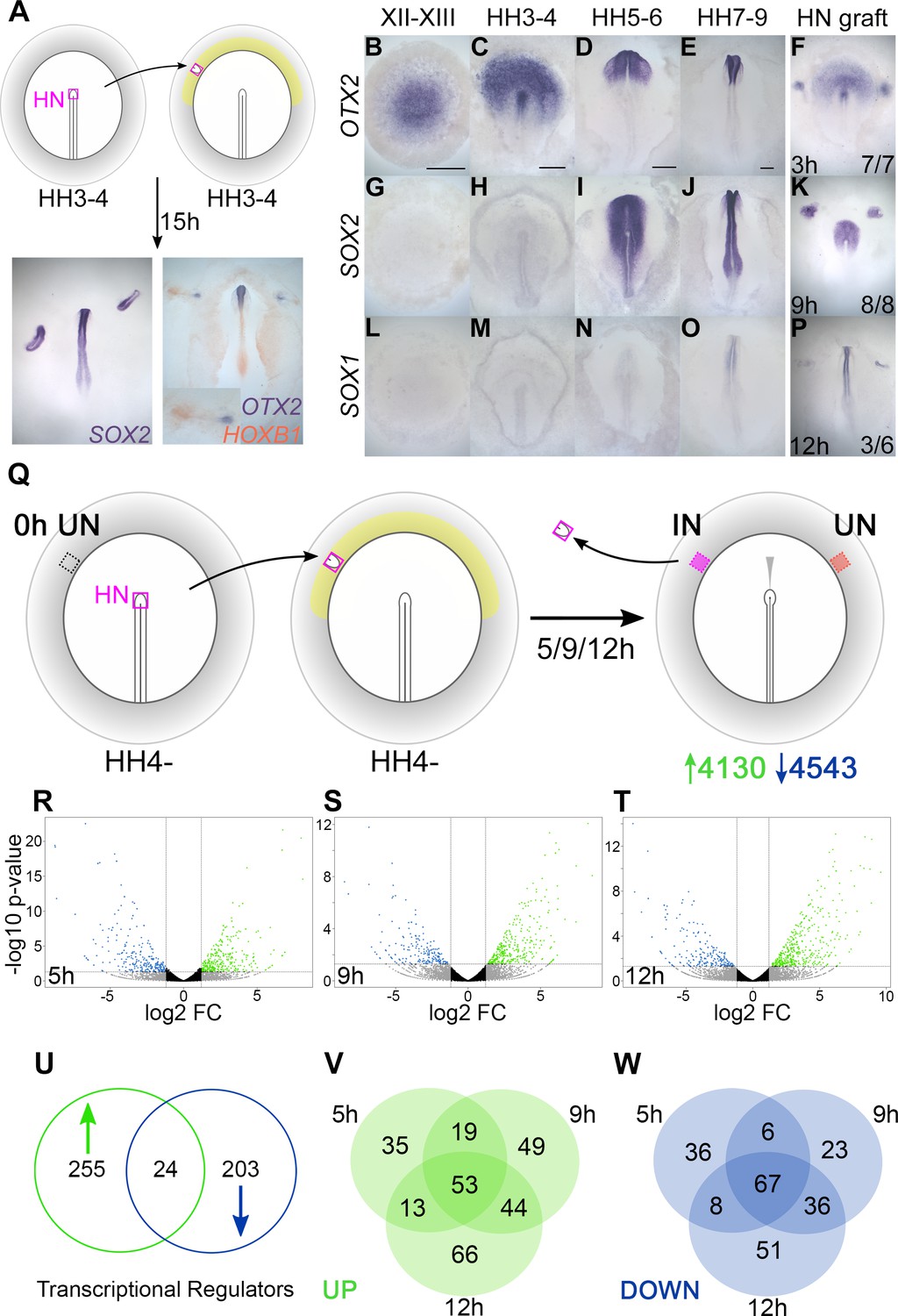
In the chick embryo, a graft of Hensen’s node to the inner area opaca, an extraembryonic region of competent non-neural ectoderm (Gallera and Ivanov, 1964; Dias and Schoenwolf, 1990; Storey et al., 1992; Streit et al., 1998), induces the formation of a mature, patterned neural tube after about 15 hr of culture from the host ectoderm (Figure 1A). To characterize the events over this period, the induction of several neural markers was assessed. OTX2 is first expressed in the pre-primitive-streak stage epiblast at EGKXII-XIII (Albazerchi and Stern, 2007; Pinho et al., 2011) and is induced by 7/7 grafts after 3 hr (Figure 1B–F). SOX2 is first expressed at HH4+/5 (Rex et al., 1997; Streit et al., 1997; Streit et al., 1998; Sheng et al., 2003) and requires 9 hr for induction (8/8) (Figure 1G–K). SOX1 starts to be expressed weakly in the neural plate around HH7-8 (Stavridis et al., 2010; Uchikawa et al., 2011) and is induced by 50% of grafts after 12 hr (Figure 1L–P). This time course confirms that a sequence of events occurs in response to a grafted node over 0–12 hr (Figure 1—figure supplement 1A), culminating in the acquisition of neural plate/tube identity (Streit et al., 1997; Streit et al., 1998; Streit and Stern, 1999; Streit et al., 2000; Sheng et al., 2003; Stern, 2005; Albazerchi and Stern, 2007; Papanayotou et al., 2008; Gibson et al., 2011; Pinho et al., 2011; Papanayotou et al., 2013; Trevers et al., 2018).

Figure 1 with 1 supplement see all

Download asset Open asset

Transcriptional profiling identifies responses to neural induction in time course.

(A) Hensen’s node (HN) was grafted from HH3-4 donors to the inner area opaca (yellow) of hosts at the same stage. An ectopic neural tube expressing *SOX2*, *OTX2,* and *HOXB1* is induced after 15 hr of culture. (**B–F**) Expression of neural markers compared to their time course of induction by a node graft: *OTX2*; first expressed in pre-streak epiblast (EGKXII-XIII) and induced by grafts after 3 hr. (**G–K**) *SOX2*; first expressed in the neural plate at HH5-6 and induced after 9 hr. (**L–P**) *SOX1*; first expressed in the forming neural tube at HH7-8 and induced after 12 hr. (Q) Identifying transcriptional responses to a node graft. HN was grafted from HH4- donors to HH4- hosts. The HN graft was removed and underlying ‘induced’ (IN) and contralateral ‘uninduced’ (UN) ectoderm isolated after 5, 9, or 12 hr. Uninduced ‘0 hr’ ectoderm from HH4- embryos was also dissected. Samples were analysed by RNA-sequencing (RNAseq). (**R–T**) Induced and corresponding uninduced tissues were compared at each time point to identify differentially expressed transcripts. Volcano plots show upregulated (green) and downregulated (blue) transcripts. (**U–W**) Venn diagrams of 482 genes encoding transcriptional regulators (U) that are upregulated (V) or downregulated (W) at different time points. Scale bars: B: 1mm; C: 250 μm; D: 250 μm; E: 250 μm. These scale bars apply to all other figures with embryos at equivalent stages throughout the paper.

Figure 1—source data 1 RNAseq galGal3 analysis key and differentially expressed transcripts.: https://cdn.elifesciences.org/articles/73189/elife-73189-fig1-data1-v2.xlsx
Download elife-73189-fig1-data1-v2.xlsx
Figure 1—source data 2 RNAseq galGal4 analysis key and differentially expressed transcripts.: https://cdn.elifesciences.org/articles/73189/elife-73189-fig1-data2-v2.xlsx
Download elife-73189-fig1-data2-v2.xlsx
Figure 1—source data 3 Nanostring probe codeset.: https://cdn.elifesciences.org/articles/73189/elife-73189-fig1-data3-v2.xlsx
Download elife-73189-fig1-data3-v2.xlsx

To uncover genes whose expression changes over this period, we performed RNAseq of the responding tissue at three time points following a graft of Hensen’s node: 5 hr (to identify early ‘pre-neural’ responses), 9 hr (when SOX2 expression defines neural specification), and 12 hr, as the host tissue starts to express SOX1. Hensen’s node was grafted from HH4- chick donors to a region of competent epiblast (inner area opaca) of chick hosts at the same stage. Embryos were cultured for the desired period of time, after which the graft was removed and the underlying ‘induced’ tissue was collected. Control (‘uninduced’) ectoderm from the corresponding region on the contralateral side of the same embryos (Figure 1Q) was also collected, as well as competent area opaca at HH4-, representing a ‘0 hr’ starting point for the time course. When ‘induced’ and ‘uninduced’ reads at each time point are compared by DESeq analyses, 8673 differentially expressed transcripts were identified (see volcano plots, Figure 1R–T). Of these, 4130 were upregulated (enriched in ‘induced’ tissue) and 4543 were downregulated (depleted in ‘induced’ tissue) relative to the ‘uninduced’ counterpart.

To construct a GRN we focused on 482 transcription factors and chromatin modifiers that are differentially expressed within these data. Of these ‘transcriptional regulators’, 255 are upregulated, 203 are downregulated, and 24 have more complex expression dynamics (Figure 1U and Figure 1—figure supplement 1B). Grouping transcripts based on the timing of their response (Figure 1V–W) reveals that 120 are differentially expressed throughout (53 upregulated and 67 downregulated), while others are associated with particular time points. Therefore, transcriptional responses to organizer grafts involve changes in the expression of many genes over a relatively short period.

Due to this complexity, we chose to increase the time resolution of the analysis. NanoString nCounter was used to quantify the gene expression changes of transcriptional regulators at six time points (1, 3, 5, 7, 9, and 12 hr after the node graft) in ‘induced’ tissue compared to ‘uninduced’ ectoderm. By consolidating the data from RNAseq and NanoString, a set of refined expression profiles was established for 213 transcriptional regulators – 156 that are enriched and 57 that are depleted in induced tissues (Figure 3—source data 1). These represent the core components of our GRN.

Epigenetic changes identify chromatin elements associated with neural induction

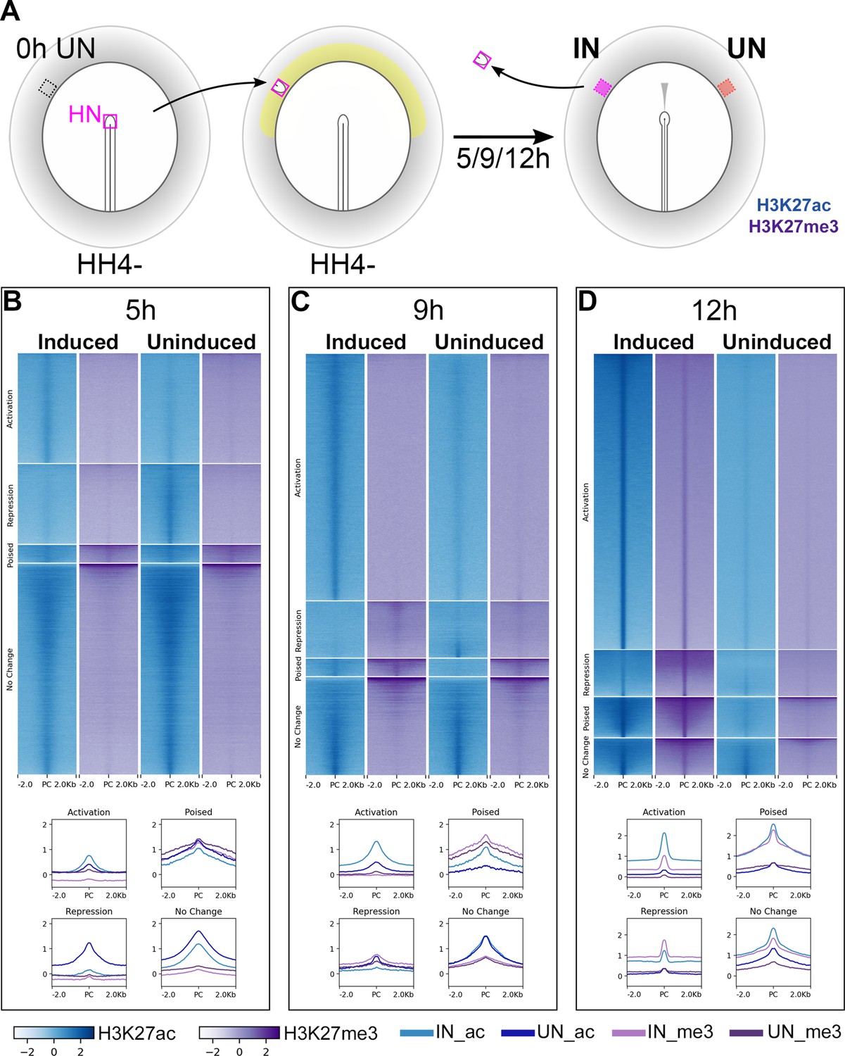
We next sought to identify the regions of non-coding chromatin that govern these transcriptional responses to signals from the organizer. Histone modifications can regulate gene expression by altering chromatin structure. For example, H3K27ac is associated with actively transcribed genes and their enhancers, whereas transcriptionally inactive regions are often marked by H3K27me3 (Tiwari et al., 2008; Heintzman et al., 2009; Creyghton et al., 2010; Kharchenko et al., 2011; Rada-Iglesias et al., 2011; Tolhuis et al., 2011; Zentner et al., 2011; Bonn et al., 2012). Therefore, ChIPseq and ATACseq (Buenrostro et al., 2013; Buenrostro et al., 2015; Corces et al., 2017) were performed on induced and uninduced ectoderm following 5, 9, or 12 hr of a node graft, to detect histone and chromatin conformation changes during neural induction.

H3K27ac and H3K27me3 enriched chromatin (ChIPseq) were identified genome-wide by comparison to matched genomic input samples. Chromatin sites were then categorized according to their histone signatures across induced and corresponding uninduced tissues at each time point (Figure 2—figure supplement 1A). Sites that become acetylated and/or demethylated in induced tissues, compared to uninduced, were considered to undergo ‘activation’ (Indices 1–3) while those that become deacetylated and/or methylated undergo ‘repression’ (Indices 4–6). Chromatin marked by both H3K27ac (activation) and H3K27me3 (repression) marks in either tissue were described as ‘poised’ (Indices 7–12). The remaining indices (13–16) define sites that do not change marks between the two conditions.

Chromatin sites undergoing activation are enriched for H3K27ac marks in induced tissues at each time point (Figure 2B–D). Sites of repression are more varied: those belonging to this category at 5 hr lose acetylation, whereas several sites become methylated in induced tissues at 9 and 12 hr. Very few sites are ‘poised’ at any time. Overall, as neural induction progresses, the number of sites undergoing activation increases, along with a reduction in those that do not change state. In contrast, ATACseq suggests that there is little difference between induced and uninduced samples in terms of chromatin accessibility (Figure 2—figure supplement 2) at 5 hr, but the differences become more marked at later time points. At 12 hr, the ATACseq profile resembles that of the endogenous neural plate of the embryo (Figure 2—figure supplement 2).

Figure 2 with 3 supplements see all

Download asset Open asset

Epigenetic changes identify chromatin elements associated with neural induction.

(A) Hensen’s node (HN at HH4-) was grafted to hosts of the same stage. Embryos were cultured for 5, 9, or 12 hr before HN was removed and induced (IN) and contralateral uninduced (UN) ectoderm collected. ChIPseq was performed for H3K27ac and H3K27me3. (**B–D**) Putative regulatory sites were predicted according to the H3K27 profiles of IN and UN tissues at each time point (see Figure 2—figure supplement 1). They include sites undergoing ‘activation’ or ‘repression’, being ‘poised’, or showing no change. Heat maps illustrate the enrichment of H3K27ac (blue) and H3K27me3 (purple) in IN and UN tissues within ±2.0 kb from the peak centre (PC) for each annotated group. Graphs plot the distributions of H3K27ac and H3K27me3 enrichment for each group.

Figure 2—source data 1 ChIPseq tissue dissociation details.: https://cdn.elifesciences.org/articles/73189/elife-73189-fig2-data1-v2.xlsx
Download elife-73189-fig2-data1-v2.xlsx
Figure 2—source data 2 ATACseq indices.: https://cdn.elifesciences.org/articles/73189/elife-73189-fig2-data2-v2.xlsx
Download elife-73189-fig2-data2-v2.xlsx

Next, we focused on epigenetic changes associated with the 213 genes encoding transcriptional regulators for which refined expression profiles were established by NanoString analysis (see above). ‘Constitutive’ CTCF-bound sites (putative insulators) flanking these genes were obtained from chicken CTCF-ChIPseq data (Khan et al., 2013; Kadota et al., 2017). They were used to predict the boundaries within which we considered H3K27 marks as being associated with the gene of interest; these regions (‘loci’) are up to 500 kb in length and may contain several genes (Figure 2—figure supplement 1B). Within each locus, the H3K27ac or H3K27me3 enriched peaks were categorized as before (Figure 2—figure supplement 1A). The 213 selected loci contain a total of 6971 sites that change in response to a node graft (Indices 1–10; Figure 2—figure supplement 1A). We noticed that the flanking regions (proximal promoters) of transcriptional regulators whose expression increases are enriched for H3K27ac marks in induced tissue (Figure 2—figure supplement 3). In contrast, there is no difference between H3K27ac and H3K27me3 marks around the flanking regions of repressed transcriptional regulators at 5 and 9 hr – they only become enriched for methylation at 12 hr. Our analysis therefore identifies putative regulatory elements that are controlled epigenetically during the process.

A GRN for neural induction

Having identified transcriptional responses to signals from the organizer and their accompanying chromatin changes, we combined them to construct a GRN to describe the time course of these events and to illustrate predicted interactions between transcriptional regulators. The open source platform BioTapestry (Longabaugh et al., 2005; Longabaugh et al., 2009; Paquette et al., 2016) (http://www.biotapestry.org) is used extensively to provide a visually intuitive representation of developmental networks (Davidson, 1990; Arnone and Davidson, 1997; Davidson et al., 1998; Betancur et al., 2010; Simões-Costa and Bronner, 2015; Thiery et al., 2020). Importantly, this software allows dynamic changes in the interactions between regulators and their target genes to be represented.

A BioTapestry model for regulatory gene interactions

To integrate these complex time course data into a GRN that models the interactions during neural induction, we developed a custom computational pipeline (Figure 3). The 213 transcriptional regulators previously identified were selected as candidate components of the network because of their responses to a node graft in both RNAseq and NanoString data, and their associated chromatin changes in ChIPseq. Interactions were predicted by screening putative regulatory sites that belong to Indices 1–3 and 7 (activation) (Figure 2—figure supplement 1C–E) for the presence of putative binding sites for transcription factors that are differentially expressed in the dataset, and expressed at the appropriate time point to fit with a putative regulatory role (i.e. simultaneously or just before) for the target locus.

Figure 3

Download asset Open asset

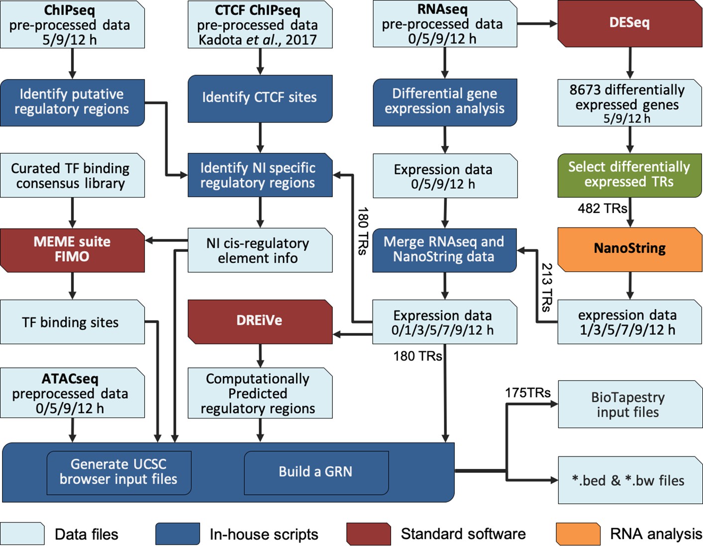
Constructing a BioTapestry model for regulatory gene interactions: computational workflow.

Computational pipeline to combine transcriptomic and epigenetic time course data, to build a gene regulatory network (GRN) for neural induction. The output data are available to view in the UCSC browser.

Figure 3—source data 1 Integrated GRN gene expression profile.: https://cdn.elifesciences.org/articles/73189/elife-73189-fig3-data1-v2.xlsx
Download elife-73189-fig3-data1-v2.xlsx

We then used the regulatory rules shown in Figure 4A–B to predict positive or negative regulatory events between regulators and their putative targets, overlaying the predicted transcription factor binding profiles with the time course of expression from RNAseq and NanoString. At each time point, changes in expression of a putative regulator that could lead to the same change in a candidate target are represented as positive interactions. Negative, or inhibitory, interactions are predicted when changes in expression of the regulator could cause the opposite change in a downstream target. Genes lacking both regulatory inputs and outputs with other genes in the network were excluded.

Figure 4

Download asset Open asset

Constructing a BioTapestry model for regulatory gene interactions: the regulatory logic.

(A) Network interactions were modelled using chromatin sites that belong to Indices 1–7 and the defined rules between regulators and their potential targets. At sites that become active in induced tissues (Indices 1, 2, 3, and 7): positive interactions are depicted when a putative input and its target are co-regulated and negative (inhibitory) interactions are modelled when an input and its target have opposing expression profiles. These rules are reversed at sites that undergo repression in induced tissues (Indices 4, 5, and 6) except that interactions are not predicted when the potential regulators of these repressed sites are not expressed. (B) Schematic depicting how expression and chromatin profiles were combined to predict interactions between gene regulatory network (GRN) components. (i) RNA-sequencing (RNAseq) and NanoString expression data provide a list of 213 transcriptional regulators that are upregulated (genes A, C, and X) or downregulated (genes B, D, and Y) after 0, 1, 3, 5, 7, 9, or 12 hr of a node graft. (ii) For these candidate GRN components, CTCF-ChIPseq data was used to predict neighbouring CTCF-bound domains of up to 500 kb. (iii) Within these, sites that are enriched for H3K27ac or H3K27me3 were identified by ChIPseq performed on induced and uninduced tissues at 5, 9, or 12 hr. (iv) Chromatin sites were categorized (according to Figure 2—figure supplement 1A) and those belonging to Indices 1, 2, 3, and 7 were selected to build a network. (v) These were screened for transcription factor binding motifs that correspond to other GRN components. This identifies genes A and D as potential regulators of target X and genes B and C as potential regulators of target Y. (vi) At each time point, the consequence of interactions was predicted according to the regulatory rules in A. Positive interactions are depicted when a putative input and its target are co-regulated. Negative (inhibitory) interactions are modelled when an input and its target have opposing expression profiles. (vii) Predicted interactions are modelled in BioTapestry using arrows for positive interactions and blunt ends for inhibitory interactions. Components are shown in colour at time points when they are expressed or shaded grey when they are not. (C) A GRN comprising 5614 predicted interactions between 175 components is visualized using BioTapestry. Each component is coloured by the time point when it first starts to express at 0 hr (purple), 1 hr (grey-blue), 3 hr (blue), 5 hr (green), 7 hr (yellow), 9 hr (orange), and 12 hr (red).

Figure 4—source data 1 List of GRN transcription factor binding sites within regulatory sites at 5h, 9h and 12h following a node graft.: https://cdn.elifesciences.org/articles/73189/elife-73189-fig4-data1-v2.xlsx
Download elife-73189-fig4-data1-v2.xlsx

The resulting GRN (Figure 4C), depicting interactions between 175 genes, was represented using BioTapestry (Supplementary file 1 and Supplementary file 2). Most targets are predicted to receive multiple positive and/or negative inputs, which are initiated at, and can act across, multiple time points. For example, the non-neural gene GATA2 is predicted to be repressed by TFAP2C after just 1 hr of a node graft, followed by increasing repression via HIF1A, MEIS2, and numerous other factors over the remaining time course. On the other hand, BLIMP1 is predicted to be induced by TFAP2C after 1 hr, alongside SNAI1, ETV1, ETV4, MGA, and SOX4 (Supplementary file 2). In total, 5614 interactions are predicted to occur between these components, highlighting the intricate and highly dynamic sequence of regulatory events that are triggered by signals from the organizer.

Incorporating individual regulatory sites and their dynamics into the network

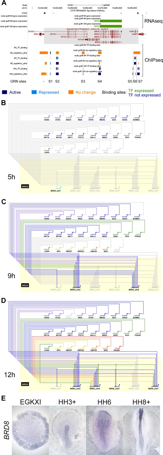
BioTapestry networks usually represent each gene once, with multiple regulatory inputs, and each regulator as a single input into the target gene. However, it is now known that gene expression is controlled by multiple elements, each with characteristic spatial and temporal activity. In the past, such elements were identified within non-coding regions that are conserved across species by testing their ability to direct appropriate expression in vivo. This approach was used, for example, to identify many enhancers controlling SOX2 expression (Uchikawa et al., 2003; Okamoto et al., 2015) – the spatiotemporal pattern of expression of most developmentally regulated genes is likely to be controlled by multiple elements. Our epigenetic analysis predicts that in almost all cases there are indeed multiple putative regulatory sites associated with genes that change expression, which can be in different chromatin states (Figure 5A). To illustrate the contributions of different chromatin elements, we generated a subnetwork for BRD8, which is located in a relatively gene sparse locus with only a few putative regulatory elements associated with it. The changes that occur as sites undergo epigenetic ‘activation’ or ‘repression’ (using Indices 1–7; Figure 4A) were modelled across the 12 hr time course. Since BioTapestry lacks a notation for discrete regulatory elements of individual genes, the subnetwork shows seven candidate cis-regulatory regions of BRD8 (BRD8_site1-BRD8_site7 in Figure 5B) at 5, 9, and 12 hr represented as separate targets (Figure 5B–D). This depicts which specific elements contain binding sites for each regulating transcription factor. One element (BRD8_site1 in Figure 5B) is initially acetylated; however, it does not seeem to receive inputs from other GRN components. This site is then methylated at 9 and 12 hr as a number of other elements become active, presumably to stabilize and maintain BRD8 expression. In situ hybridization (Figure 5E) confirms that BRD8 is not expressed in the pre-primitive-streak stage epiblast (EGKXII) or in the prospective neural plate at HH3-4. BRD8 expression becomes enriched later in the neural plate and neural tube, as predicted by the network regulatory dynamics. This subnetwork illustrates the complexity of regulatory dynamics that underlie gene expression even at a relatively simple locus. Although it is not practical to represent the entire network including all the elements in their different states in this way using BioTapestry, all identified elements and their predicted activity are presented in the associated UCSC browser tracks (https://genome.ucsc.edu/s/stern_lab/Neural_Induction_2021), together with the predicted binding sites relevant to the network contained within each site; a full list is also given in Figure 4—source data 1.

Figure 5

Download asset Open asset

A subnetwork incorporating individual regulatory sites and their dynamics.

(A) UCSC browser view of RNA-sequencing (RNAseq) and ChIPseq tracks associated with *BRD8. BRD8* is upregulated after 9 and 12 hr of neural induction (green bars). The *BRD8* regulatory locus (grey box; chr13:10028086–10091079) is defined by flanking CTCF-bound sites. Seven putative regulatory sites (S1-7) within this domain were predicted based on the ChIPseq H3K27 profiles. This includes sites that undergo activation (Indices 1–3, 7, coloured in dark blue), repression (Indices 4–6, coloured in cyan), or show no change (coloured in orange). Transcription factor binding sites by network components are shown; green for components that are expressed at the same time point and blue for those that are not. A BioTapestry subnetwork was generated from these predicted binding sites and expression profiles. Site 3, active at 12 hr, is not shown in the subnetwork as there is no TF that is expressed at 12 hr and predicted to bind to it. (B) *BRD8* regulation during neural induction: *BRD8* is initially not expressed; site 1 is active but is not predicted to be bound by other gene regulatory network (GRN) components. Each GRN component is coloured according to the time point when it first starts to express at 0 hr (purple), 1 hr (grey-blue), 3 hr (blue), 5 hr (green), 7 hr (yellow), 9 hr (orange), and 12 hr (red). (C) *BRD8* is upregulated after 9 hr; sites 2 and 6 undergo activation and could be bound by various transcription factors that are also expressed. Site 1 undergoes repression. (D) *BRD8* expression is maintained at 12 hr; regulators potentially bind to sites 2, 4, 5, and 7. Site 6 is no longer predicted to be active. (E) In situ hybridization detects BRD8 transcripts in the neural plate at HH6 and neural tube at HH8+, but not at earlier stages, EGKXI and HH3+.

Prediction of core transcriptional regulators of the network

Genes with high ‘outdegrees’ and ‘betweenness centralities’ are often considered to be ‘core genes’ in a network. The ‘outdegree’ of a network component A is the number of outgoing interactions from component A to other components in the network (including component A itself), whereas the ‘betweenness centrality’ of a network component A is a measurement that captures the importance of component A based on the frequency at which interactions between pairs of other genes do so only by passing through component A (White and Borgatti, 1994). To predict key hubs in the network that may play more important roles during the process of neural induction, we calculated the ‘outdegrees’ and ‘betweenness centralities’ of network components across seven time points (0, 1, 3, 5, 7, 9, and 12 hr) (Figure 6). In the 0 hr network, ESRRG, GRHL2, and TFAP2A appear to be core genes in ectoderm cells prior to their exposure to a node graft (Figure 6B). Soon after grafting a node, these genes are immediately downregulated and repressed, with predicted repressive inputs from the core genes in the GRN. At the 1 hr time point following a node graft, TFAP2C, SOX4, and BLIMP1 start to be expressed and are predicted to act as core genes, acting as repressors of the next layer of core genes in ectoderm cells (Figure 6C–E). Other predicted neural induction core genes, such as SOX3, TCF12, and MYCN, are highlighted as key transcriptional regulators acting throughout the process of neural induction at multiple time points (Figure 6D–H), and are predicted to bind to the enhancers of many genes in the GRN.

Figure 6

Download asset Open asset

Identifying core regulatory factors in the neural induction gene regulatory network (GRN).

(A) Correlation between the number of regulatory output (outdegree) and the degree of centrality of genes. (**B–H**) Network interactions at 0, 1, 3, 5, 7, 9, and 12 hr. The size of a node indicates the degree of the centrality of a gene. The degree of regulatory outputs is represented with the following colour scheme: red, orange, yellow, and green indicate high, medium, to low degree of regulatory outputs.

Neural induction by a graft of Hensen’s node recapitulates normal neural plate development

To what extent is the induction of an ectopic neural plate by an organizer graft comparable to the events of neural plate development in the embryo? To address this, we used three complementary approaches. First, we explored the spatial and temporal expression patterns of network components during normal embryo development. Then, we conducted scRNAseq analysis of stages of neural plate development concentrating on network components and their temporal hierarchical organization. Finally, we tested the activity of several of the putative regulatory elements in normal embryos to assess whether their activity in the neural plate in vivo resembles the hierarchy revealed by node grafts.

Spatiotemporal expression of GRN components during normal neural plate development

A previous study identified genes whose expression differs between EGKXII-XIII (pre-primitive-streak) epiblast, neural plate at HH6-7, and non-neural ectoderm (Trevers et al., 2018). When these embryonic tissues (Figure 7A) are compared to neural induction, we find that the pre-streak epiblast is most similar to induced ectoderm after 5 hr of a node graft, while 9 and 12 hr time points are more closely related to mature neural plate (Figure 7B). This encouraged us to generate a detailed spatiotemporal map of transcripts during embryonic neural plate development. Genes that are differentially expressed in induced tissues compared to uninduced in RNAseq were selected. In situ hybridization was performed for 174 transcriptional regulators (including 123 that are represented in the GRN) at four stages: pre-streak (EGKXII-XIII), primitive streak (HH3-4), head process/early neural plate (HH5-6), and neural fold/tube (HH7-9).

Figure 7 with 8 supplements see all

Download asset Open asset

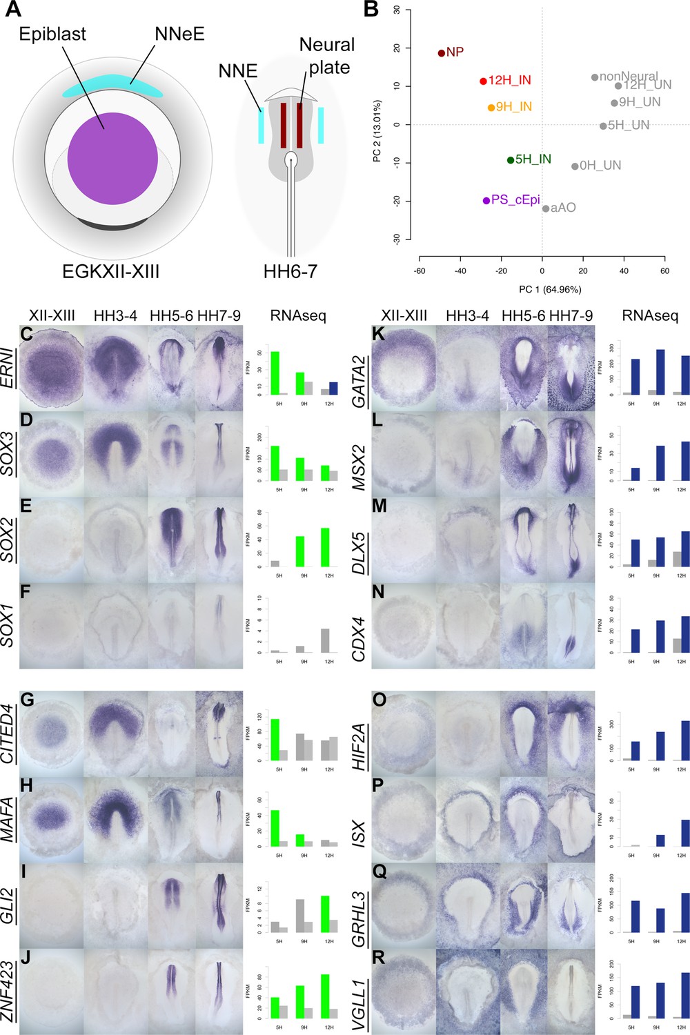
A spatiotemporal map of the normal embryo for transcripts differentially expressed during neural induction.

(A) Central epiblast from pre-primitive-streak stage embryos (PS_cEpi) at EGKXII-XIII, neural plate (NP) at HH6-7, and corresponding non-neural extraembryonic ectoderm were dissected and processed by RNA-sequencing (RNAseq). (B) Principal component analysis comparing prospective neural and non-neural tissues from the normal embryo to induced (IN) and uninduced (UN) ectoderm 5, 9, or 12 hr after a node graft. (**C–R**) In situ hybridization of genes encoding transcriptional regulators at four stages of embryonic development (EGKXII-XIII, HH3-4, HH5-6, and HH7-9) compared to their RNAseq expression after 5, 9, and 12 hr of a node graft. Bar charts plotted RNAseq values (FPKM) in induced and uninduced tissues. Bars are shaded green when genes are upregulated in induced tissue (FPKM >10 in induced tissue and fold change (FC) >1.5 compared to uninduced). Bars are shaded blue when genes are downregulated (FPKM >10 in uninduced tissue and FC <0.5 compared to uninduced). When a gene is neither upregulated nor downregulated, the bars are coloured in dark grey in induced and light grey in uninduced. Genes represented within the neural induction GRN are underlined.

Figure 7—source data 1 Sumary of changes for upregulated transcriptional regulators based on in situ expression patterns.: https://cdn.elifesciences.org/articles/73189/elife-73189-fig7-data1-v2.xlsx
Download elife-73189-fig7-data1-v2.xlsx
Figure 7—source data 2 Summary of changes in downregulated transcriptional regulators based on in situ expression patterns.: https://cdn.elifesciences.org/articles/73189/elife-73189-fig7-data2-v2.xlsx
Download elife-73189-fig7-data2-v2.xlsx
Figure 7—source data 3 Details of probes generated by digestion of cDNAs that were used for in situ hybridisation.: https://cdn.elifesciences.org/articles/73189/elife-73189-fig7-data3-v2.xlsx
Download elife-73189-fig7-data3-v2.xlsx
Figure 7—source data 4 Details of probes generated by PCR that were used for in situ hybridisation.: https://cdn.elifesciences.org/articles/73189/elife-73189-fig7-data4-v2.xlsx
Download elife-73189-fig7-data4-v2.xlsx
Figure 7—source data 5 PCR primer sequences.: https://cdn.elifesciences.org/articles/73189/elife-73189-fig7-data5-v2.xlsx
Download elife-73189-fig7-data5-v2.xlsx

There is a striking correspondence between neural induction by a node graft and normal neural development in terms of the spatiotemporal patterns we observed. In addition to confirming the expression of known neural markers (ERNI, SOX3, SOX2, and SOX1; Figure 7C–F), the predictions from node grafts uncover many novel responses such as CITED4 (ERNI-like), MAFA (SOX3-like), GLI2, and ZNF423 (SOX2-like) (Figure 7G–J). In total, 84/89 transcriptional regulators that are induced by a node graft were detected in neural tissues at some stage (Figure 7 and Figure 7—figure supplements 1–4). Only 5 of the 89 genes (HEY1, RFX3, STOX1, TAF1A, and ZIC2) could not be detected by in situ hybridization – these are expressed at very low FPKM levels according to RNAseq. Most of the transcriptional regulators that are induced by a node graft (79/84) have not previously been associated with neural induction (Figure 7—source data 1). Likewise, a high proportion (65/85; 76%) of the transcripts that are downregulated after a node graft are depleted in neural tissues relative to non-neural territories. Among these are known non-neural markers such as GATA2 and MSX2 and the extraembryonic marker HIF2A (Figure 7K, L and O). Neural/non-neural border markers (such as DLX5, MSX1, and TFAP2C; Figure 7M and Figure 7—figure supplements 5–8) were also downregulated, supporting suggestions that neural induction involves the repression of an early border identity (Trevers et al., 2018). We also uncover several other genes (such as ISX, GRHL3, and VGLL1) that are excluded from neural tissues (Figure 7P–R).

This approach reveals even subtle temporal changes in expression. For example, CITED4 is sharply upregulated after 5 hr of a node graft but is later downregulated (Figure 7G). In the embryo, it is expressed in pre-streak epiblast and prospective neural plate at HH3-4, but CITED4 transcripts are then absent from the neural plate at HH5-6. CDX4 (Figure 7N) and HOXA2 (Figure 7—figure supplement 6J) are initially repressed by a node before their expression levels increase at 12 hr – just as they become enriched in the posterior neural tube from HH7-9. These observations confirm that transcriptional responses to a node graft closely follow the events that occur during development of the embryonic neural plate of the normal embryo.

The GRN describes a temporal hierarchy occurring in single cells during neural development

To follow the expression of multiple genes during normal neural plate development and to compare this to the temporal hierarchy of our GRN, we assessed the expression of network components in individual cells at different stages of normal neural development. scRNAseq was performed on ectoderm dissected from chick embryos at HH4, HH6, HH8, and HH9+. These broad regions included prospective or mature neural plate and neural tube as well as non-neural ectoderm and neural plate border (Figure 8A).

Figure 8 with 1 supplement see all

Download asset Open asset

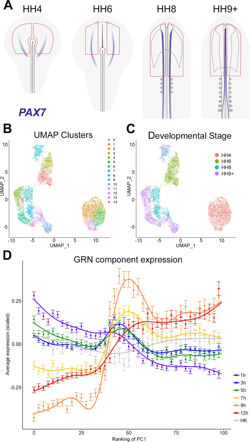
The gene regulatory network (GRN) describes a temporal hierarchy occurring in single cells during neural development.

(A) Broad regions of prospective neural plate, neural plate border and non-neural ectoderm were dissected at HH4, HH6, HH8, and HH9+ and processed for single-cell RNA-sequencing (scRNAseq). *PAX7* expression marks the border between neural and non-neural tissues. (B) UMAP displaying unbiased clustering of cells into 15 clusters (0–14) representing distinct cell identities. (C) UMAP displaying the developmental stage from which the cells were collected; cells from HH4 and HH6 form independent clusters, whereas HH8 and HH9+ are more intermixed. (D) Temporal hierarchy of expression of GRN components in single cells during neural plate development. Prospective neural plate and neural tube cells (clusters 0, 1, 2, 5, 6, 7, 9, 13, and 14) were selected and ranked according to PC1 (see Figure 8—figure supplement 1C). The average gene expression (mean ± SE) is plotted for groups of components that are induced at each time point in the GRN, compared to housekeeping genes (HK). A general additive model was fitted to visualize the smoothed expression profile across the ranking of PC1 (using bins of 2.5).

The non-linear dimensionality reduction method UMAP was then used for unbiased cell clustering in low dimensionality space (Figure 8B). Cells collected from the two earliest developmental stages (HH4 and HH6) each form a distinct group, whereas cells from later stages (HH8 and HH9+) cluster primarily according to identifiable cell populations (Figure 8C). Cell identities were assigned to the 15 clusters using well-established markers (Figure 8—figure supplement 1A). This revealed groups corresponding to placodal (cluster 8), neural crest (clusters 10, 11), and neural tube identities (clusters 4, 6, 7, 9, 13, 14) within the HH8 and HH9+ cell populations. At HH6, neural plate cells expressing LIN28B, SETD2, and SOX2 (cluster 0) are distinct from non-neural plate progenitors (cluster 3), which express GATA2, DLX5, and TFAP2A. At HH4, prospective neural cells express MAFA, ING5, and LIN28B (clusters 1, 2, and 5) whereas cluster 12 expresses the node marker ADMP.

To identify groups of genes that are co-expressed across the entire dataset, gene module analysis was performed using Antler (Delile et al., 2019). Cell state-specific modules were then selected by applying the criterion that at least 50% of the genes in a module must be differentially expressed (log fold change (FC) >0.25, FDR <0.001) in at least one cell cluster relative to the rest of the dataset. This defines 17 distinct modules (Figure 8—figure supplement 1B), which support our cell type classifications. Module-3 shows co-expression of PAX2, WNT4, and NKX6-2 and is upregulated in prospective midbrain clusters 9 (at HH8) and 6 (at HH9+). Module-10 is defined by co-expression of PAX7, SOX8, SOX10, and TFAP2B and is associated with neural crest (clusters 10, 11). Module-25 has low levels of expression of GATA2 and ID3 (clusters 1, 2, 5, 12) at HH4, which are then further downregulated at later stages, except in non-neural cells at HH6 (cluster 3) and placodal cells at HH8 (cluster 8).

To explore the temporal hierarchy of GRN components, we assessed their expression in prospective neural plate and neural tube cell populations (clusters 0, 1, 2, 4, 5, 6, 7, 9, 13, 14). Within the ‘neural’ population, principal component (PC) analysis (PCA) revealed that PC1 inversely correlates with developmental stage (Figure 8—figure supplement 1C), therefore cells were ranked according to their position along PC1 to explore temporal expression dynamics. To visualize the expression of GRN components, genes were grouped according to the time point at which they are first induced by a node graft; their average (normalized and scaled) expression was then plotted (Figure 8D). This analysis reveals that components upregulated within 1–5 hr of a node graft are initially highly expressed in prospective neural cells and that their expression decreases progressively across PC1. GRN components that are induced after 7–12 hr are expressed at higher levels later, in cells of the maturing neural plate and neural tube. Therefore, GRN components identified from node graft experiments are expressed in a temporal hierarchy that closely replicates normal neural plate development.

Responses to neural induction reveal enhancers that drive neural gene expression during normal development

Do the regulatory elements predicted by the GRN generated from Hensen’s node grafts correspond to those that regulate normal development of the neural plate in the embryo? To define the putative enhancers more precisely, we combined our histone profiling (Figure 2 and Figure 2—figure supplement 1) and ATACseq (Figure 2—figure supplement 2) to identify regions of open/active chromatin from induced and uninduced tissues after 5, 9, and 12 hr after a node graft. These regions were then compared to ChIPseq (for H3K27ac/me3) and ATACseq performed on pre-primitive-streak epiblast and mature neural plate at HH6-7.

We chose six putative enhancers for more detailed exploration. These were identified within the previously described CTCF loci using the overlapping combination of H3K27ac marks and ATACseq reads to predict enhancers that are likely to be active (Figure 9—figure supplements 1–3) based on the indices and expression profiles as described earlier. Each region was cloned into the pTK-EGFP vector (Uchikawa et al., 2003) to drive GFP expression via a minimal promoter; the reporter was then electroporated into the pre-primitive-streak stage (EGKX-XI) epiblast or a broad region including the prospective neural plate at HH3/3+ (Figure 9A) and embryos cultured for 5 hr or to the desired stages.

Figure 9 with 3 supplements see all

Download asset Open asset

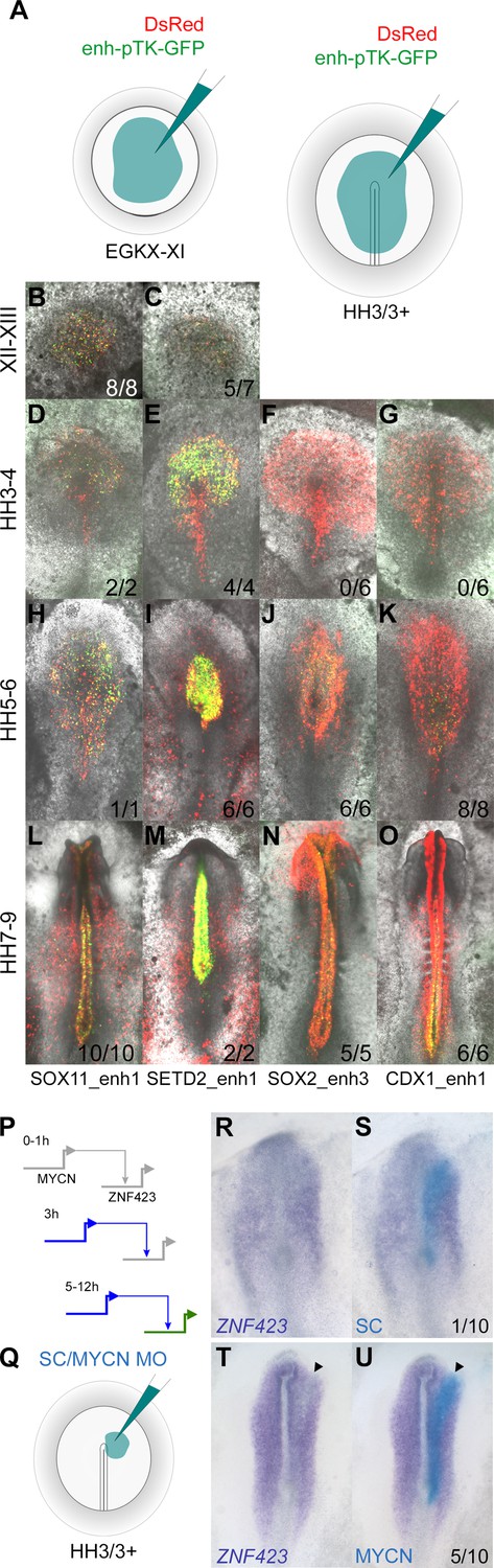
Enhancers identified by the neural induction assay have activity consistent with the expression of the gene during normal neural plate development.

(A) Putative enhancers were cloned into the E-pTK-EGFP vector and co-electroporated into a broad region of the pre-streak stage (EGKX-XI) or HH3+ epiblast together with DsRed. (**B–C**) Activity of SOX11_enh1 and SETD2_enh1 at EGKXII-XIII; (**D–G**) activity of SOX11_enh1, SETD2_enh1, SOX2_enh3, and CDX1_enh1 at HH4; (**H–K**) HH5-6; (**L–O**) HH7-9. (**P–U**) Effect of knockdown of predicted network targets by electroporation of a morpholino (MO): a MYCN MO knocks down the expression of predicted target ZNF423, compared to a control MO.

Figure 9—source data 1 Sequences of primers used for cloning enhancers.: https://cdn.elifesciences.org/articles/73189/elife-73189-fig9-data1-v2.xlsx
Download elife-73189-fig9-data1-v2.xlsx

Each enhancer drives neural-specific GFP expression in a spatiotemporal pattern strikingly similar to the gene that lies in its proximity (Figure 9B–O and Figure 9—figure supplements 1–3). For example, SOX11_enh1 and SETD2_enh1 are enriched for H3K27ac in induced tissues after 5 hr (Figure 9—figure supplement 1A–B). Both are active in the epiblast at EGKXII-XIII and prospective neural plate at HH3-4, when SOX11 and SETD2 are expressed (Figure 9—figure supplement 1 C-AY). SOX2_enh3 is ‘poised’ after 5 hr of neural induction, but acquires an active signature at 9 hr when it gains H3K27ac and ATAC reads (Figure 9—figure supplement 2A). As expected, this enhancer is not active in the prospective neural plate at HH4 (Figure 9—figure supplement 2C–H); GFP positive cells are detected later when SOX2 is expressed in the neural plate proper at HH5-6 (Figure 9—figure supplement 2I–N). Likewise, GLI2_enh1 and SIX3_enh2 also become active after 9 hr; GLI2_enh1 is detected throughout the neural plate, whereas SIX3_enh2 is restricted to the forming forebrain at HH6 (Figure 9—figure supplement 3A–Z). These five enhancers remain active in the neural tube in correspondence with H3K27ac marks and ATAC reads that persist after 12 hr of a node graft.

CDX1_enh1 is also active in the caudal neural tube at HH7-9, when it also weakly labels some presomitic mesoderm cells. Its activity is detected at HH5-6, but only in a few cells of the caudal lateral epiblast adjacent to Hensen’s node and not in the neural plate (Figure 9—figure supplement 2U -AL). This sparse activity overlaps closely with the discrete region from which neuro-mesodermal precursors (NMPs), which are said to express CDX1 (Gouti et al., 2017), are thought to contribute to both neural and somite tissues (Brown and Storey, 2000; Tzouanacou et al., 2009). Since the CDX1 gene is expressed earlier (HH3-4), but only in mesoderm and primitive streak, the activity of this enhancer is likely to be associated with NMPs.

Therefore, the domain of reporter activity for all six predicted enhancers corresponds to that of the normal expression of the associated gene. Furthermore, the stage at which the reporter first becomes active closely matches the stage at which the gene starts to be expressed during normal development.

Finally, to validate predictions from the network, we tested the interaction between MYCN (one of the core network genes; Figure 6A), which is upregulated from 3 hr, and its predicted target ZNF423, which is upregulated at 5 hr onwards (Figure 9P). Electroporation of a morpholino against MYCN into the prospective neural plate at HH3/3+ (Figure 9Q) knocks down the expression of ZNF423 (Figure 9R–S; 5/10 embryos), which is usually expressed later in the neural plate and neural tube (Figure 7J), compared to a control morpholino (Figure 9T–U; 1/10 embryos).

Taken together, these comparisons between node grafts and normal embryos strongly suggest that histone profiles that change in response to a node graft (upon which our network is based) can predict regulatory elements relevant to neural development. This establishes our GRN as a robust tool to describe the genetic hierarchy associated with the acquisition of neural identity.

Browser resources

In addition to the BioTapestry GRN and other associated data described above, the results of this project, including data from node grafts in time course and from normal neural plate development, are made available on the UCSC browser at https://genome.ucsc.edu/s/stern_lab/Neural_Induction_2021. This incorporates RNAseq, ChIPseq, and ATACseq for all expressed and repressed genes (not limited to GRN components) and the annotated putative regulatory regions with predicted binding sites for GRN components. Finally, to help to predict potential conservation of the regulatory sites across species, we performed DREiVe analysis (Sosinsky et al., 2007; Khan et al., 2013; Streit et al., 2013) for domains within a 500 kb window around each of the genes represented in the GRN, using human (hg38), mouse (mm10), rat (rn6), golden eagle (aquChr2), zebrafish (danRer10), and chicken (galGal5). Blocks of sequence with conserved motifs are included as a track in the browser.

Discussion

Although neural induction was first described a century ago, it has often been thought of almost as a discrete switch, changing the fate of cells as they respond to a signal or signals emanating from the ‘organizer’. This study reveals a much greater complexity of responses to signals from the organizer, in very fine time course up to the time of appearance of mature neural plate markers. We show that the hierarchy of responses to a graft of Hensen’s node into a remote part of the embryo closely recapitulates the events of normal neural plate development, including not only the timing of gene expression in the developing neural plate, but also appropriate spatiotemporal activity of enhancers identified by the graft assay. Our GRN, comprising 175 transcriptional regulators and 5614 putative regulatory interactions between them, describes neural induction in unprecedented detail and allows us to predict the consequences of manipulating the activity of these components. This represents the most comprehensive example to date of a detailed network in a vertebrate embryo, modelled on both transcriptional and chromatin changes that take place in vivo, at high temporal resolution.

An important feature that distinguishes our approach from many others in the current literature is that we are able to monitor events in a known, precise time course relative to the time of exposure of the responding tissue to the organizer. This is only possible because of our experimental design: grafting the organizer into a region that does not normally give rise to the neural plate (but is able to do so in response to the graft) provides a clear ‘time-zero’, to act as reference. Thereafter, we have undertaken the time course at relatively short intervals, collecting transcriptional profiles at 0, 1, 3, 5, 7, 9, and 12 hr after the graft and epigenomic data at four of these time points (0, 5, 9, and 12 hr). It represents one of the most refined transcriptomic and epigenomic analyses of a developmental process studied in vivo and reveals the complexity of changes that can occur even over a relatively brief period. By performing our analysis on carefully dissected responding tissue (rather than a large portion or even a whole embryo), the resulting network should therefore be less subject to ‘noise’ from other events unrelated to the responses of competent cells to signals from the organizer. Since the fine temporal resolution reveals the ‘direction’ (e.g. increasing or decreasing) of expression changes at each time point, it is possible to identify concomitant changes in neighbouring non-coding chromatin and to predict their role in transcriptional activation or repression. Along with this, we can also observe changes in expression of transcription factors that have binding sites within those regions. These features make it possible to predict the GRN in a virtually unsupervised manner, using the workflow described.

Is neural induction by a grafted organizer comparable to normal neural plate development?

Although a graft of Hensen’s node is able to induce a neural plate, neural tube and their subsequent patterning into forebrain, midbrain, hindbrain, and spinal cord, as well as neural crest and placodes from the host epiblast of the area opaca, this is probably not how the process of central nervous system (CNS) development proceeds in the normal embryo. For a start, a large proportion of the cells that will form part of the neural plate (corresponding to the most cranial regions, forebrain, midbrain, and most of the hindbrain), never appear to be in close proximity to the node or anterior primitive streak. This implies that signals from tissues other than the node or streak are likely to play a role, especially at the earliest stages of neural development. We have shown that neural plate development is likely to start very early, before primitive streak formation, and probably under the initial influence of the hypoblast, involving FGF signals (Streit et al., 2000; Trevers et al., 2018). Therefore, although the node can induce an entire CNS including the earliest steps (as it also expresses FGF8), this is not what happens in normal development.

A second important issue arises by considering the formal definition of induction: ‘an interaction between one (inducing) tissue and another (responding) tissue, as a result of which the responding tissue undergoes a change in its direction of differentiation’ (Gurdon, 1987). The ‘change in the direction of differentiation’, in more contemporary terms, might be described as a ‘change of fate’ or ‘change in tissue identity’. By implication, to conclude that an inductive interaction takes place, we first need to define an inducing tissue (source of signals), the outcome of the induction (the final identity/fate resulting from the interaction) and importantly, a responding tissue whose normal fate, in the absence of induction, should not be the same as the outcome – otherwise there would be no ‘change’. This means that it is not possible to determine whether the prospective neural plate of the normal embryo develops as a result of one or more inductive interactions, especially since we cannot determine the earliest stage at which the first inducing signals are presented to that responding tissue.

For these reasons, the time course initiated by a transplanted tissue that is able to induce a complete nervous system in a responding tissue whose fate is not to form a neural plate is an invaluable tool to study the acquisition of neural plate identity. Here, we have taken advantage of this approach by first constructing a GRN with a fine time course in a competent responding tissue after such a transplant, defining the hierarchy and dynamics of expression of more than 150 transcription factors and other markers, along with changes in chromatin marks that accompany this. Then, we addressed the question of whether this hierarchy of events is in any way comparable to what occurs during normal neural development, using three complementary approaches:

First, using in situ hybridization for the majority of genes contained in the GRN, noting the time and location of their initial expression, we assessed whether markers upregulated by a node graft are expressed in the normal neural plate, and whether those repressed by a graft become excluded from the neural plate, and from what stage. This was then compared with the order of events after a node graft. We found a very strong correspondence: genes whose expression is induced by a node graft within 3 hr tend to be expressed in the pre-primitive-streak stage embryo (around stage EGK XIII), those induced at 5–7 hr in the central area pellucida anterior to and around the node at stages 4–6, and those induced at 9–12 hr are expressed in the elevating neural plate from stages 7–9, confirming previous observations made with just a few genes (Figure 1 and Figure 1—figure supplement 1).

Second, we generated reporters for a subset of the predicted enhancers from the GRN, containing a minimal promoter (TK), the putative enhancer, and the coding sequence of GFP. This was co-electroporated into a wide region of the early embryo along with a vector encoding a fluorescent protein under the control of a strong ubiquitous promoter (DS-Red-Express) to mark the entire territory that had been electroporated. We then assessed the area within the electroporated territory (red from DS-Red) where the enhancer was active (green from GFP). In all six cases examined, the domain of expression corresponded to that of the normal expression of the associated gene, and the stage at which the reporter first became active closely matched the stage at which the gene starts to be expressed.

Finally, we compared gene expression of the neural plate/tube and the neural plate border in the normal embryo at single-cell level at four stages of development (primitive streak stage HH4, head fold stage HH6, four-somite stage HH8, and nine-somite stage HH9+; the time interval between each pair of these stages of normal development is approximately 2–3 hr). Dimensionality reduction and unsupervised clustering revealed clusters of cells representing neural plate and its different anterior-posterior parts, non-neural ectoderm, neural crest, and placodal cell states. Modelling transcriptional dynamics of components of the GRN across inferred pseudo-time revealed a very close correspondence between normal neural plate development and the sequence of transcriptional changes which take place following a node graft.

Taken together, these three approaches all strongly indicate that the sequence of events that characterize the response of area opaca epiblast cells to a graft of the organizer closely follows the dynamics of gene expression in the normal neural plate.

The network – interpreting enhancer states

Our analysis reveals thousands of sites across the genome containing marks that change with the progression of neural induction. Each locus contains genes whose expression changes during this cascade, and their associated putative regulatory elements. As previously described for other systems such as embryonic stem (ES) cells in culture, regulatory elements may be decorated simultaneously by marks associated with activation (e.g. H3K27ac) and with repression (e.g. H3K27me3); these have been called ‘poised’ or ‘bivalent’ enhancers (Cui et al., 2009; Heintzman et al., 2009; Xu et al., 2009; Creyghton et al., 2010) and have been interpreted to indicate that the site is in transition from one state to the other, or perhaps able to go either way. Our fine time course reinforces this concept; in many cases we observe that cells pass from one state (e.g. H3K27me3 without acetylation) to the opposite, sometimes passing through a ‘poised’ state at the intermediate time point. This could suggest that these changes can occur sequentially in a cell. However, other interpretations are also possible. One possibility is that the apparent contradictory marks are due to different modifications of the two alleles of the locus in question, which could also be a transitional state. Another possibility is that this progression may reflect cells within a tissue that do not undergo the change synchronously, but some cells start earlier than their neighbours, the tissue gradually becoming more homogeneous. This sort of progression is sometimes seen by in situ hybridization or time-lapse movies of reporter activity (e.g. to visualize the activity of enhancer N2 associated with the SOX2 gene [Uchikawa et al., 2003; Papanayotou et al., 2008]). Likewise, in the present paper, SOX11 expression begins as a mosaic (salt-and-pepper) in the early pre-streak epiblast before becoming more homogeneous, and the activity of the SOX11_enh1 (Figure 9—figure supplement 1C–H) shows a similar pattern at the same stage. Most likely these apparently ‘poised’ or ‘bivalent’ sites reflect a combination of these reasons.

Among the many regulatory elements predicted by our analysis are some that have been described previously (Uchikawa et al., 2003; Uchikawa et al., 2011; Okamoto et al., 2015; Iida et al., 2020). Their analysis was based on conserved stretches of non-coding sequence, followed by testing the activity of fragments in a vector containing a heterologous minimal promoter. In some cases, there are differences in the length of the sequence considered to act as an enhancer by both studies. For example, our SOX2_enh3 partially overlaps with, and its behaviour upon electroporation mimics the activity of, the previously identified SOX2 D1 enhancer (Okamoto et al., 2015; Iida et al., 2020). Therefore, our ChIPseq analysis can verify known enhancers as well as identifying many new candidates.

Calculations of ‘outdegrees’ and ‘betweenness centralities’ of the components in the network across seven time points (0, 1, 3, 5, 7, 9, and 12 hr) reveals a relatively small subset of transcriptional regulators with high values in both parameters (Figure 6). These are defined as ‘core genes’ (or ‘network hubs’) in the network and may play more important roles during the process of neural induction. We tested whether one of these, MYCN, is required to regulate its predicted target, ZNF423 at the appropriate time point (Figure 9R–S) using morpholino electroporation. The knockdown reduced expression of the target gene in a significant proportion of embryos, confirming MYCN as a regulator of ZNF423 expression. However, it is worth considering that in the case of other enhancers such as the N2 element of SOX2, it appears that no single TF binding to the element is individually essential – rather, several TFs need to bind but the precise combination may not be so critical (Uchikawa et al., 2003; Uchikawa et al., 2011; Okamoto et al., 2015; Iida et al., 2020). This may be a general feature of such developmentally regulated elements, therefore testing whether a factor is ‘essential’ can give a misleading view of gene regulation in the biological context being studied.

Can the network help to illuminate developmental concepts?

The GRN has great complexity over a relatively short period of time, with many transcription factors changing their expression and thousands of predicted interactions between them undergoing concomitant changes. We initially expected that a detailed view of the responses to signals from the organizer might somehow highlight specific changes, or states, that could be associated with some of the key concepts of developmental biology, such as ‘induction’ and ‘commitment’ (Slack, 1991; Stern, 2004) to a neural plate identity. These concepts have classically been defined based on specific embryological manipulations but it has hitherto not been possible to identify specific molecular signatures associated with these transitions. Could we use the present GRN to find objective molecular criteria that correspond to such changes in developmental properties?

Based on timed organizer grafts followed by their removal, a critical time was established at 12–13 hr after a graft (Gallera and Ivanov, 1964; Gallera, 1965; Gallera, 1971b; Gallera, 1971a), using similar conditions to those of our node grafts here. At this time point, removal of the node graft does not impair the subsequent development of the neural plate. This represents the endpoint of our GRN; at this time SOX2 is robustly expressed, and SOX1 is just starting to be expressed, in the responding tissue (Pevny et al., 1998). Although this functional assay does not test for ‘irreversibility’ of the cell fate transition, the finding that only after this point it can proceed autonomously without further signals from the organizer suggests that this time point might correspond to at least some degree of ‘commitment’ (or ‘determination’) to a neural plate identity.

Another earlier study has defined an initial state (named the ‘common state’) reflecting the earliest responses (1–3 hr) to a node graft into the area opaca (Trevers et al., 2018). A similar state is elicited by a graft of lateral head mesoderm (which induces placodes) and by a graft of the node (which induces the CNS), and the genes comprising this ‘common state’ have some similarity to those expressed by ES cells. In normal embryos, these genes are expressed in a broad region of the embryonic epiblast; moreover, a graft of the hypoblast into the area opaca also induces a similar set of genes. These observations suggested that the responses to inducing tissues start by a ‘rewinding’ (or reprogramming) cells to a state similar to that of the very early embryonic epiblast, from where cells can then be redirected to their new fate: neural plate, placode, neural crest, epidermis, and perhaps others. A similar state can also be elicited by exposure of area opaca to a source of FGF8 (a factor normally secreted by both the hypoblast and the node, but lost by the node at the time when its inducing ability starts to decline; Storey et al., 1992; Streit et al., 2000).

Functional studies have established that competent ectoderm cannot respond to BMP inhibitors like Chordin unless it has previously been exposed to a graft of the organizer for at least 5 hr (Streit et al., 1998). This led to the identification of a few genes whose expression is associated with this transition (Streit et al., 2000; Sheng et al., 2003; Gibson et al., 2011; Pinho et al., 2011; Papanayotou et al., 2013), but the present experiments greatly expand and enrich this by placing genes in the context of a comprehensive network of gene interactions. Future experiments can take advantage of this information to determine the mechanisms that cause epiblast cells to become sensitive to BMP inhibition at this time point, and the upstream signals responsible.

To define possible ‘key’ steps, if they exist, we have attempted to identify ‘core’ factors that appear to represent important hubs in the GRN and their downstream targets and interconnections (Figure 6). This revealed a small number of genes that appear to occupy nodal, highly connected, positions in the network, and include, at successive time points, ESRRG, GRHL2, and TFAP2A in epiblast not exposed to a graft (0 hr) but then almost immediately downregulated, then TFAP2C, SOX4, and BLIMP1 just 1 hr after a node graft. Indeed, BLMP1 (PRDX1) has recently been shown to be required transiently at an early stage for neural plate, crest, and placode development, and its subsequent downregulation is also essential for further differentiation (Prajapati et al., 2019). Other later putative core genes include SOX3, TCF12, and MYCN. Future experiments could address whether these do indeed represent key steps accompanying neural induction. For the time being, we feel that functional definitions of the developmental concepts will remain key to defining the properties of developing tissues, especially given the complexity of the changes in gene expression accompanying neural induction.

Does ‘neural induction’ occur in the normal embryo, and if so when and how?

The gene signature that defines the ‘common state’ is induced by a graft of Hensen’s node after approximately 3 hr. The same genes are expressed in the epiblast of the normal embryo before primitive streak formation (stage EGK XIII), long before the node has formed; they can be induced by a graft of the hypoblast, as well as by the node. This suggests that in the normal embryo, it is the hypoblast rather than the node that initiates this process (Foley et al., 2000; Streit et al., 2000; Trevers et al., 2018). However, a node graft can mimic both these initial steps and those that follow. Therefore, although a node graft is able to generate a complete neural plate when grafted into a region of competent epiblast that normally does not give rise to this tissue, neural plate development in the normal embryo is likely to be directed by signals emanating from more than one tissue. A large part of the prospective CNS (forebrain, midbrain, and anterior hindbrain) is never close to the node but extends far anteriorly from the primitive streak. Indeed it has been suggested that the most anterior nervous system may be induced by signals other than the node, as well as earlier in development, and that the node and its derivatives may be involved mainly in the induction of the more caudal parts of the CNS (posterior hindbrain and spinal cord) (Beddington, 1994; Thomas and Beddington, 1996; Foley et al., 2000; Streit et al., 2000; Metzis et al., 2018). Armed with the GRN presented here, it will be particularly interesting in future to assess which sub-modules (‘kernels’) of the GRN are regulated by which secreted factors expressed in the node and whether and when similar factors are also normally expressed in other tissues that display partial or full neural induction activity.

Neural induction in vivo and in vitro

A growing literature makes use of protocols to direct cultured mouse ES cells or human induced pluripotent stem cells into neurons, and calls this process ‘neural induction’. After maintaining the stem cell population in a medium containing FGF to sustain proliferation and pluripotency, a common current protocol involves withdrawal of the FGF, followed by activation of the hedgehog pathway (Gouti et al., 2014; Metzis et al., 2018). Other protocols in the literature include BMP inhibition, manipulation of the Wnt pathway, and/or retinoid signalling, in various combinations. Almost all of these protocols need at least 5 days, and sometimes as long as 14 days, for the culture to generate neuronal cells. This is a much longer period than we see in vivo, which raises the question of to what extent they represent equivalent processes. Our network should help to compare them and to assess the degree of similarity as well as identify any differences. We have already shown that the initial (‘common’) state in response to induction (the first 3 hr or so in our assays) generates a state comparable to ES cells, suggesting that the remaining part of the differentiation protocols correspond to the period after this.

Conclusion, and a resource to assess conservation among the vertebrates

In conclusion, our study provides the first GRN to represent the changes that accompany the process of neural induction after grafting an organizer to an ectopic site, and how it relates to normal neural plate development, in fine time course. We provide a comprehensive resource (deposited in the UCSC genome browser) that includes not only the network components (transcriptional regulators with predicted cross-regulatory interactions), but also a genome-wide view of all transcriptional changes, H3K27 acetylation/methylation, and chromatin conformation (ATACseq) during this process, from the time cells are initially exposed to neural inducing signals to the time at which definitive neural plate markers start to be expressed. We envisage that the GRN and the accompanying resource will be invaluable tools to study other important aspects of early neural development, such as the signalling inputs responsible for these changes, the molecular basis of the competence of cells to respond to neural inducing signals at different locations and stages, and aspects of neural patterning leading to regional diversification of the CNS. We also envisage that this resource will be useful to understand the process of neural induction not only in the chick but also in other vertebrate species, as well as in protocols for neural differentiation in ES cells in vitro. Indeed, we have noticed that out of 84 upregulated genes included in this network, the majority (74/84) are expressed in the prospective mouse neural plate (Figure 7—source data 1). These 84 genes include 69 not previously associated with neural induction in any species, of which the majority (56/69) are expressed in the future mouse neural plate. These observations suggest a high degree of evolutionary conservation. To aid in cross-species comparisons and possible studies on evolutionary changes that have occurred in neural induction, the browser resource also includes the results of computational prediction of conservation of the key GRN loci among several vertebrate species, using DREiVe, a computational tool designed to identify conserved sequence motifs and patterns rather than precise sequence conservation (Sosinsky et al., 2007; Khan et al., 2013; Streit et al., 2013).

Materials and methods

Chicken eggs and embryo culture

Request a detailed protocol

Fertile hens’ eggs (Brown Bovan Gold; Henry Stewart & Co., UK), were incubated at 38°C in a humidified chamber to the desired stages. Embryos were staged according to Hamburger and Hamilton, 1951, in Arabic numerals or Eyal-Giladi and Kochav, 1976, in Roman numerals for pre-primitive streak (pre-streak) stages. Embryos were harvested and dissected in Pannett-Compton saline (Pannett and Compton, 1924) or 1× PBS, before being fixed in 4% paraformaldehyde (PFA) overnight at 4°C or prepared for ex ovo culture. All experiments were conducted on chicken embryos younger than 12 days of development and therefore were not regulated by the Animals (Scientific Procedures) Act 1986.

Chicken embryos were cultured ex ovo using a modified New culture method (New, 1955; Stern and Ireland, 1981) as previously described (Voiculescu et al., 2008). In brief, eggs were opened and the thin albumin was collected. Intact yolks were transferred to a dish containing Pannett-Compton saline. The vitelline membrane was cut at the equator while keeping the embryo central. The membrane was then slowly peeled away from the underlying yolk to keep the embryo attached. Membranes were placed on a watch glass with the embryo orientated ventral side up. A glass ring was positioned over the embryo and the edges of the membrane wrapped over the ring. This assembly was then lifted out of the dish and adjusted under a dissecting microscope while keeping the embryo submerged in a small pool of saline. The vitelline membrane was gently pulled taut around the glass ring before the excess was trimmed. Excess yolk was cleared from the membrane and embryo by gently pipetting a stream of saline and then replaced with fresh liquid, leaving the embryo on an optically clear membrane. At this point, embryos can be cultured as they are or with the addition of a node graft which were transferred to the ring and positioned while the embryo is submerged. To complete the culture, saline was removed from around and within the ring without disturbing the embryo and grafts. The dry ring was then transferred to a 35 mm Petri dish containing a shallow pool of thin albumin. The edges of the ring were pressed down to prevent it from floating, leaving the embryo supported by a shallow bubble of albumin beneath the membrane. Completed cultures were incubated in a humidified chamber at 38°C for the desired length of time. After culture, embryos were fixed on the membrane with 4% PFA or submerged with ice-cold saline to allow tissue dissection.

Neural induction assays

Request a detailed protocol

Neural induction assays were performed as previously described (Stern, 2008; Streit and Stern, 2008). For Hensen’s node grafts, chick donors and hosts at Hamburger-Hamilton (HH) 3+/4- were used and New cultures incubated for 1, 3, 5, 7, 9, or 12 hr at 38°C in a humidified chamber. One or two nodes were grafted per embryo, placed contralaterally within the inner third of the area opaca, at or above the level of the host node. This region is competent to respond to neural inducing signals but only contributes to the extra-embryonic membranes and not the embryo proper (Streit et al., 1997). Nodes were grafted with their endodermal surface in contact with the host epiblast.

RNAseq tissue collection and processing

Request a detailed protocol

For RNAseq, HH4- chick nodes were grafted to the area opaca of HH4- chick hosts. A single node was grafted to the left or right side per host, and embryos were cultured for 5, 9, or 12 hr. Node grafts were removed by submerging the embryo in saline while still attached to the membrane. Fine syringe needles (27 G or 30 G, BD Microlance) were used gently to lift the grafted tissue away from the underlying epiblast. Where grafts were firmly attached, 0.12% trypsin dissolved in saline was gently pipetted over the graft site to assist in removal. After dissection, trypsin activity was neutralized by treating embryos briefly with heat-inactivated goat serum (Stern, 1993), which was removed by washing with fresh saline. The induced epiblast directly beneath the graft, which appeared greyish and thickened, was dissected using syringe needles and mounted insect pins. Uninduced epiblast tissue from same position on the contralateral side was also dissected. Tissue samples per condition were pooled, frozen on dry ice, and stored at –80°C. At each time point (5, 9, or 12 hr) a total of 50 induced and contralateral uninduced pieces of tissue were collected. A further 50 pieces of uninduced tissue were collected from HH4- embryos that had not been cultured, representing a 0 hr control. Tissue samples for each condition were then pooled and lysed in 1 mL TRIzol (Invitrogen) for RNA extraction.

RNA sequencing was conducted by Edinburgh Genomics (formerly ARK Genomics; Roslin Institute, University of Edinburgh, UK). Total RNA was extracted and the quality was assessed using the Agilent 2100 Bioanalyzer – all samples registered an RIN value between 9.0 and 10.0. Libraries were constructed using the Illumina TruSeq mRNA library preparation kit. In brief, mRNAs were purified using oligo-dT conjugated magnetic beads before being chemically fragmented to on average 180–200 bp. Fragments were then transcribed using short random primers and reverse transcriptase to produce single-stranded cDNA, from which double-stranded cDNA was generated by DNA polymerase I and RNase-H. After synthesis, cDNA was blunt-ended and a single A-base added to the 3’ end. Sequencing adapters were ligated via a T-base overhang at their 3’ and these libraries were then purified to remove unincorporated adapters before being enriched by 10 cycles of PCR. Library quality was checked by electrophoresis and quantified by qPCR. The seven RNA libraries were sequenced over two lanes via 100-cycle, paired-end sequencing using the Illumina HiSeq 2000 system.

Whole-mount in situ hybridization

Request a detailed protocol

Antisense riboprobes were generated from cDNA plasmid templates or Chick Expressed Sequence Tag (ChEST) clones (Source Bioscience). Templates were linearized by restriction digest (Figure 7—source data 3) or by PCR (Figure 7—source data 4) using M13 forward (5’-GTAAAACGACGGCCAGT-3’) and M13 reverse (5’-GCGGATAACAATTTCACACAGG-3’) primers (Figure 7—source data 5). The products were transcribed using SP6, T7, or T3 (Promega) and DIG-labelled nucleotides. DNA templates were digested using RNase-free DNase and the RNA probe was precipitated and resuspended in water. Working probes were diluted to 1 μg/mL in Hybridization (HYB) buffer and stored at –20°C.

Whole-mount in situ hybridization was performed as described previously (Stern, 1998; Streit and Stern, 2001), but omitting pre-adsorption of the anti-DIG-AP antibody (Roche 11633716001, used at 1:5000). Stained embryos were imaged from the dorsal perspective using an Olympus SZH10 Stereomicroscope with an Olympus DF PlanApo 1× objective and an Olympus NFK 3.3× LD 125 photo eyepiece. Images were captured using a QImaging Retiga 2000R Fast 1394 camera and QCapture Pro software as 24-bit, colour TIFF files at 300 dpi with dimensions of 1600×1200 pixels.

A spatiotemporal expression map was generated for genes that are differentially expressed after either 5, 9, or 12 hr of a node graft. These were selected from the galGal3 and galGal4 RNAseq analyses according to the criteria as described in ‘Differential expression analysis’.

NanoString tissue collection and processing

Request a detailed protocol

Uninduced tissue or induced epiblast that had been exposed to node grafts was dissected as previously described. Four to eight pieces of tissue were collected in triplicate per condition. Tissues were dissected in ice-cold 1× PBS and collected on ice. All excess solution was removed using a fine needle and promptly processed by adding a total of 1 µL of lysis buffer from the RNAqueous-Micro Total RNA Isolation kit (Thermo Fisher). Tubes were immediately snap-frozen on dry ice and stored at –80°C.

NanoString experiments were run on the nCounter Analysis System using a custom codeset and following NanoString guidelines. The codeset consisted of 386 probes (Figure 1—source data 3) belonging to various categories. Transcriptional regulators that are upregulated (coloured red) or downregulated (coloured green) at 5, 9, or 12 hr were selected from RNAseq screening (details in ‘Differential expression analysis‘). Other genes that respond to 5 hr exposure to a node graft (Streit et al., 2000; Sheng et al., 2003; Gibson et al., 2011; Pinho et al., 2011; Papanayotou et al., 2013) were also included. Probes were also designed against housekeeping genes (ACTB, GAPDH), markers of apoptosis and proliferation, transcriptional readouts of FGF, BMP, WNT, retinoic acid, Notch and Hedgehog signalling; epithelial, mesodermal, endodermal, neural plate border, pre-placodal, neural crest and Hensen’s node markers, and standard positive and negative NanoString controls.

Tissue samples were processed using the NanoString master kit and following the manufacturer’s instructions. Probes were hybridized to lysates overnight for 17 hr at 65°C before the reactions were transferred to the NanoString prep-station robot and processed using the ‘high-sensitivity’ program. Probe-target complexes were digitally counted from 600 fields of view on the NanoString Analyzer.

Enhancer cloning and electroporation

Request a detailed protocol

Enhancers were identified based on changing active, inactive, or poised chromatin signatures over 5, 9, and 12 hr of neural induction. These were referenced against the 5, 9, and 12 hr ATACseq data to select putative enhancers with accessible chromatin. The primers used for cloning are detailed in Figure 9—source data 1.

Enhancers were cloned from chick gDNA as previously described (Chen and Streit, 2015). The correct sized fragments were amplified by PCR using PCRBio Ultramix (PCRBiosystems) and ligated into the pTK_JC_EGFP plasmid (Chen and Streit, 2015) using T4 ligase (NEB). Ligation products were transformed into DH5α Escherichia coli and grown on agar plates with Ampicillin selection. Clones were screened by colony PCR using PCRBio Ultramix and pTK_Fwd (5’-GTGCCAGAACATTTCTCTATCG-3’) and pTK_Rev (5’-GTCCAGCTCGACCAGGATG-3’) primers. Positive clones were cultured overnight in 5 mL LB broth plus Ampicillin and the constructs were purified by mini-prep (Qiagen). Enhancer inserts were sequenced using Citrine_Fwd (5’-TGTCCCCAGTGCAAGTGC-3’) and Citrine_Rev (5’-TAGAACTAAAGACATGCAAATATATTT-3’) primers. Plasmids with sequence verified inserts were maxi-cultured in 200 mL, of which 1 mL used to make a 50% glycerol stock and stored at –80°C. Bulk plasmid DNA was extracted using the Endofree Plasmid Maxi-prep kit (Qiagen) following the manufacturer’s instructions and resuspended in 100 µL of sterile water. Further purification was conducted to reduce residual salts which interfere with electroporation efficiency and embryo damage. Samples were spun for 15 min/15,000 rpm/4°C to pellet any particulates. The supernatant was removed to a fresh tube, to which 10 µL of 3 M NaOAc pH 5.2 and 250 µL of 100% EtOH was added to precipitate the plasmid DNA. This was pelleted by centrifugation at 15 min/15,000 rpm/4°C and the pellet was washed with 70% EtOH and spun again for 10 min/15,000 rpm/4°C. The supernatant was removed and the pellet allowed to air-dry completely, before being resuspended in 50 µL of sterile water and the concentration checked by nanodrop and adjusted to 5 mg/mL.

Enhancer plasmids were co-electroporated with pCMV-DsRed-Express-N1 (Clontech) which labels all electroporated cells. Tissues were electroporated using an anode electroporation chamber and wire cathode according to Voiculescu et al., 2008, with minor modifications. Electroporation mix was made fresh by combining the following in water: enhancer_TK_EGFP plasmid (2 mg/mL), pCMV-DsRed-Express-N1 (1 mg/mL), 6% sucrose, 0.02% Brilliant Blue FCF. This was backloaded into a capillary needle with a fine tapered tip. The anode chamber was filled with 1× PBS and the electrodes positioned ≈2 cm apart.

Harvested embryos were positioned directly between the electrodes with the dorsal side (epiblast) upwards, closest to the cathode. Electroporation mix was applied using a mouth aspirator attached to the capillary needle, and by bringing the needle tip in close contact with the embryo. For pre-streak EGKX-XI embryos, electroporation mix was applied broadly across the central epiblast region and immediately electroporated using the following current settings: 3.5–4.0 V, 5 pulses, 50 ms duration and a 100 ms gap. At HH4- stages, electroporation mix was applied broadly across the prospective neural plate and primitive streak and immediately electroporated using 4.5–5 V, 5 pulses, 50 ms duration and 100 ms gap. After electroporation embryos were transferred to vitelline membranes, prepared for New culture and cultured to the desired stages (Voiculescu et al., 2008).

Enhancer activity was imaged using a Leica SPEinv microscope with a 5× objective and LAS-X software. Images were captured at 2048×2048 pixels, speed 400 ms, and 1× zoom with an averaging of 4. EGFP was excited using a 488 nm laser and detected with a 492–543 nm wavelength filter. DsRed was excited using a 532 nm laser and detected with a 547–653 nm wavelength filter. Files were saved as.lif format and composite images were stitched together in Fiji (Schindelin et al., 2012) using the Pairwise Stitching plugin (Preibisch et al., 2009).

Morpholino electroporation

Request a detailed protocol

Fluorescein-labelled morpholinos at 500 µM (MYCN: TCTTGCTGATCATTCCCGGCATGGC, or Standard control: CCTCTTACCTCAGTTACAATTTATA) were co-electroporated with pCMV-DsRed-Express-N1 (1 mg/mL) as a carrier. Constructs were targeted to the lateral prospective neural plate of embryos at HH3/3+ and electroporated using the following conditions: 4.0 V, 5 pulses, 50 ms duration and 100 ms gap. Embryos were then cultured overnight for 12 hr to reach stages HH5-8.

In situ hybridization was performed (as described above) to reveal ZNF423 expression using an anti-DIG-AP antibody and NBT/BCIP. Embryos were then post-fixed overnight in 4% PFA. They were then washed extensively in PBST and incubated at 70°C for 1 hr. Further PBST washes were performed to remove residual traces of NBT-BCIP. Immunohistochemistry was then performed to detect fluorescein-labelled morpholinos using anti-FITC-AP (Roche 11426338910, used at 1:5000) and BCIP alone.

ChIPseq tissue collection and processing

Request a detailed protocol

In brief, tissues were dissected in ice cold 1× PBS and transferred to low binding PCR tubes containing 50–100 µL of 1× Protease Inhibitor Cocktail in 1× PBS (cOmplete mini EDTA-free; Roche) on ice. Where necessary, 0.12% trypsin or 1× PBS + 200 mM EDTA was used to aid dissection. Treated tissues were rinsed with PBS to remove residual trypsin. Tissues were collected in batches every 30 min before tubes were spun at 100 × g/3 min/4°C to gently pellet the tissue. Tubes were snap-frozen in liquid nitrogen before storage at –80°C for up to 6 months. For pre-streak EGK XII-XIII embryos, the hypoblast was removed and central epiblast was collected from six embryos in triplicate. After removal of the underlying mesoderm and endoderm, the neural plate at HH6-7 was harvested from 20 embryos in triplicate. For 0, 5, 9, and 12 hr node induced and contralateral uninduced area opaca, 14–30 pieces of tissue were collected in triplicate. A further 60 pieces of 9 and 12 hr uninduced tissue were collected and processed separately after it was discovered that 30 pieces of uninduced tissue at these time points did not generate enough material for ChIP.

ChIP was performed by micrococcal nuclease (MNase) digestion to fragment the chromatin following a previous protocol (Brind’Amour et al., 2015), followed by immunoprecipitation according to the Low Cell ChIPseq kit (Active Motif, 53084) with some modifications. Corresponding induced and uninduced samples were processed side-by-side, each as three reactions: H3K27ac, H3K27me3, and input. In brief, 200 µL of protein G agarose beads were added to 2×1.5 mL low binding tubes and spun for 3 min at 1250 × g and 4°C. The supernatant was removed and the beads were washed with 690 µL of TE buffer at pH 8.0. These tubes were spun again for 3 min at 1250 × g and 4°C and the supernatant removed before bead blocking reactions were set up. To one tube, 200 µL of TE buffer pH 8.0, 20 µL of blocking reagent AM1 and 20 µL of BSA were added. This tube of ‘pre-clearing’ beads was incubated for 3–6 hr on a 4°C rotator. To the second tube, 180 µL of TE buffer pH 8.0, 20 µL of blocking reagent AM1, 20 µL of BSA, and 20 µL of Blocker were added. This tube of ‘IP’ reaction beads was incubated overnight on a 4°C rotator.

While beads were blocking, tissues were prepared for nuclei isolation and MNase digestion. A pair of samples (induced and contralateral uninduced) were thawed on ice for 5–10 min and the tissues pooled into one tube per condition using low binding tips. Pooled samples were spun at 100 × g/3 min/4°C and the excess supernatant was removed without disturbing the tissues, to leave ≈5 µL remaining. To each tube, 20 µL of nuclei lysis buffer was added, containing 16 µL of nuclei isolation buffer (Sigma N3408), 2 µL 1× protease inhibitor (Roche cOmplete mini, EDTA-free) and 2 µL of 1% IGEPAL CA-630. Tubes were gently tapped to mix and incubated on ice for 5 min. Nuclei were dissociated gently by pipetting 15 or 30 times without making bubbles, then incubating samples on ice for 15 min before repeating these steps four to five times as listed in Figure 2—source data 1.

Chromatin was then fragmented using MNase. This was carried out in two steps to fragment the easily digestible chromatin and then re-digest the more compact chromatin in a second longer digestion. A 3× master mix containing 169.5 µL of sterile H₂O, 30 µL of 10× MNase buffer (NEB), 30 µL of 50% PEG 6000, and 6 µL of 100 mM DTT (made fresh) was prepared. In a separate tube, 3 µL of 10× MNase buffer (NEB M0247) was diluted in 25 µL of H₂O, before adding 2 µL of MNase, to give a 1:15 dilution of MNase enzyme. Of this, 4.5 µL of MNase 1:15 was added to the 3× master mix, to give a total volume of 240 µL. Then, 50 µL of 3× MNase master mix was added to each tube containing 25 µL of isolated nuclei. The mixture was pipetted 15 times to mix without making bubbles, while tubes were kept on ice. This mixture was transferred to a fresh 0.2 mL low binding PCR tube at room temperature and the digestion incubated at room temperature for 2.5 min. This tube was returned to ice and 6 µL of 200 mM EDTA added. Tubes were spun at 500 × g and 4°C for 5 min to pellet larger undigested chromatin and the supernatant (containing smaller, readily digestible chromatin) was transferred to a fresh 1.5 mL low binding microfuge tube. A further 30 µL of the MNase master mix was added to the remaining chromatin pellets on ice and resuspended by pipetting 60 times, before tubes were incubated for 6 min at room temperature. To break up remaining nuclear debris, 4 µL of 200 mM EDTA and 4 µL of 1% TX-100 +1 % sodium deoxycholate were added and the mixture pipetted 30 times. All 38 µL of this second digestion was collated with the first supernatant and kept on ice (total volume ≈110 µL).

Once the ‘pre-clearing’ beads were ready (after 3–6 hr) they were spun for 3 min/1250 × g/4°C. The supernatant was removed and the beads washed with 665 µL of ChIP Buffer (from Active Motif kit) by inverting the tube several times. Beads were spun again for 3 min/1250 × g/4°C and supernatant removed again, before 232 µL of ChIP buffer was added. An even suspension of 100 µL of beads was added to each tube of MNase digested chromatin (≈110 µL). Then, 10 µL of proteinase inhibitor cocktail, 10 µL PMSF (from the Active Motif kit), and a further 290 µL of ChIP buffer were added, giving a total volume of 520 µL. Tubes were then placed on a rotator at 4°C for 3 hr to pull down chromatin fragments that bind non-specifically to the protein G agarose beads.

After ‘pre-clearing’, samples were spun at 3500 rpm and 4°C for 3 min and the supernatant was divided into three separate 0.5 mL low binding PCR tubes: 200 µL each into H3K27ac and H3K27me3 tubes and the rest into the input tube (≈60 µL). To the experimental tubes, 2 µL of H3K27ac (Active Motif 39133, lot# 31814008) or H3K27me3 (Active Motif 39155, lot# 31814017) antibody was added, and these were incubated overnight at 4°C. To the input, 80 µL of low EDTA TE buffer was added and stored overnight at 4°C.

The following day, ChIP reaction tubes were spun briefly at 4°C to collect the solution. ‘IP’ reaction beads were removed from the rotator and mixed to an even suspension by pipetting with a wide bore tip. Keeping the beads well mixed, 50 µL of bead slurry was added to each immunoprecipitation and the tubes returned to the 4°C rotator for 3–4 hr to pull down ChIPed chromatin. Next, samples were washed according to Section G of the Active Motif Low Cell ChIPseq manual and eluted with 100 µL of Elution Buffer AM4.

Chromatin was de-crosslinked by incubating ChIP and input samples at 65°C for 2 hr. Then, 125 µL of phenol:chloroform:isoamyl alcohol 25:24:1 and 64 µL of chloroform:isoamyl alcohol mixture was added and samples shaken vigorously for 15 s before centrifuging at 16,000 × g/15 min/4°C. The top aqueous layer was transferred to a fresh low binding tube. An additional 100 µL of nuclease free water was added to the original tube, which was shaken and centrifuged again. Then the aqueous top layer was removed and added to the first. To this, 2 µL of blue glycogen and 20 µL of 3 M NaOAc pH 5.2 were added and samples flicked to mix. Finally, 660 µL 100% ethanol was added, and tubes flicked to mix well before precipitating overnight at –20°C. The next day, the chromatin was centrifuged at 16,000 × g/30 min/4°C. Supernatant was removed and the pellet washed with 900 µL of cold 70% EtOH. The pellet was spun at 16,000 × g/30 min/4°C and washed with 70% EtOH again, a total of four times. Then, chromatin pellets were air-dried completely for 10–15 min and resuspended in 20 µL of TE low EDTA buffer overnight at 4°C, before being stored at –20°C until library preparation.

ChIPseq library preparation

Request a detailed protocol

Libraries were prepared using the Next Gen DNA Library kit (Active Motif 53216) and Next Gen Indexing kit (Active Motif 53264) but using ProNex size-selective beads (Promega) to enrich for mono- and di-nucleosomes (≈200–500 bp). Each sample of ChIPed chromatin was thawed on ice, to which 20 µL of low EDTA TE Buffer was added. For each library, ‘Repair 1’ reaction mix was prepared according to the Active Motif manual by combining 13 µL of low EDTA TE, 6 µL of Buffer W1, and 1 µL of Enzyme W2. This was added to the 40 µL of chromatin and mixed by pipetting. Reactions were incubated for 10 min at 37°C in a thermocycler with the lid open. To clean up the reaction, 180 µL (3× volume) of evenly suspended ProNex beads were added and incubated for 10 min at room temperature before placing on a magnetic rack for 5 min. The supernatant was removed and beads were washed three times with 100 µL of wash buffer, for 30–60 s each. The final wash buffer was removed and the beads were air-dried for 5 min. Next, Repair II reactions were prepared by combining 30 µL of low EDTA TE, 5 µL of Buffer G1, 13 µL of Reagent G2, 1 µL of Enzyme G3, and 1 µL of Enzyme G4. This was added to dry beads and pipetted to mix. Tubes were incubated on a thermocycler for 20 min at 20°C with lid open. Next, 90 µL (1.8× volume) of PEG NaCl was added to each reaction and mixed by pipetting 15 times. Samples were incubated at room temperature for 10 min and then on the magnetic rack for 5 min and beads washed and air-dried as before. Next, Ligation I mix was prepared by combining 20 µL of low EDTA TE, 3 µL of Buffer Y1, and 2 µL of Enzyme Y3, which was added to each tube of dry beads and mixed by pipetting. To each sample, 5 µL of Y2 index was added to uniquely barcoded libraries. Reactions were mixed by pipetting 60× and incubated in a thermocycler for 15 min at 25°C with the lid open. To clean up, 39 µL (1.3×) of PEG NaCl was added to each tube and mixed by pipetting 15×. Samples were incubated for 10 min at room temperature and 5 min on a magnetic rack, before beads were washed and air-dried as before. Ligation II mix was prepared by combining 30 µL of low EDTA TE, 5 µL of Buffer B1 2 µL of Reagent B2-MID, 9 µL of Reagent B3, 1 µL of Enzyme B4, 2 µL of Enzyme B5, and 1 µL of Enzyme B6. This was added to the dried beads and mixed by pipetting 30×, before incubating in a thermocycler for 10 min at 40°C with the lid open. Then, 55 µL (1.1×) of PEG NaCl was added and mixed by pipetting 30×. Samples were incubated for 10 min at room temperature and 5 min on a magnetic rack before beads were washed and air-dried as before. DNA was eluted by adding 50 µL of elution buffer and pipetting 15×. Tubes were incubated tubes at room temperature for 5 min, and then on a magnetic rack for 5 min. The eluate was transferred to a clean tube and the beads washed with a further 10 µL of elution buffer. This was collected and combined with the first 50 µL of eluate.

DNAs were size-selected using 1.2×/0.4× ratios of ProNex beads to purify ≈200–500 bp fragments. First, 72 µL of ProNex beads were added to the eluate and mixed by pipetting 30×. Samples were incubated for 10 min at room temperature and for 5 min on a magnetic rack. The supernatant (containing fragments <500 bp) was transferred to a clean tube. Then, a further 24 µL of ProNex beads were added to this supernatant and mixed 30× by pipetting. This was incubated for 10 min at room temperature followed by 5 min on a magnetic rack. The supernatant was removed and beads (with DNA fragments >200 bp bound) were washed three times with 100 µL of wash buffer, each time soaking beads for 30–60 s. The final wash buffer was removed and beads air-dried for 5 min. DNA was eluted by adding 10 µL of low EDTA TE, pipetting 10× to mix, and incubating for 10 min at room temperature. After 5 min on a magnetic rack, the eluate was transferred to a fresh tube and the beads incubated for a further 10 min with 10 µL of TE. This was collected and combined with the first collection to give a total of 20 µL.

Libraries were amplified by adding amplification mix containing 10 µL of low EDTA TE, 5 µL of Reagent 1, 4 µL of Reagent 2, 10 µL of Buffer R3, and 1 µL of Enzyme R4 to each tube. This was mixed by pipetting and incubated on a thermocycler using the following conditions: Denature1 – 98°C for 30 s, Denature2 – 98°C for 10 s, Anneal – 60°C for 30 s, Extension – 68°C for 60 s, Repeat to Denature2 for total 13 cycles, Final extension – 68°C for 60 s, Soak – 4°C forever.

Libraries were purified by adding 75 µL (1.5× volume) of ProNex beads and pipetting 60×. Samples were incubated at room temperature for 10 min, and 5 min on a magnetic rack. The supernatant was discarded and beads washed three times with 100 µL of wash buffer, before being air-dried for 5 min. Libraries were finally eluted in 20 µL of TE and their quality checked by Tapestation. They were sequenced by 75 bp single end reads to a depth of ≈20 million reads per library using the NextSeq 500 system.

ATACseq tissue collection and processing

Request a detailed protocol

OMNI-ATACseq was conducted according to Corces et al., 2017, with some adjustments, which was in turn based on Buenrostro et al., 2013; Buenrostro et al., 2015. In brief, 0, 5, 9, and 12 hr node induced and contralateral uninduced tissues were dissected in ice-cold 1× PBS and transferred to low binding PCR tubes containing 1× Protease Inhibitor Cocktail in 1× PBS (cOmplete mini EDTA-free; Roche) on ice. Where necessary, 0.12% trypsin was used to aid dissection, and treated tissues rinsed with 1× PBS to remove residual trypsin activity. Tissues were collected in batches every 30 min before tubes were spun at 100 × g/3 min/4°C to gently pellet tissues. Tubes were snap-frozen in liquid nitrogen before storage at –80°C for up to 4 months. At each time point, 14–22 pieces of tissue were collected in duplicate.

Once sufficient tissues were collected, they were thawed on ice and the nuclei isolated in 2 mL of 1× Homogenization Buffer Unstable (HBU) with a Dounce homogenizer on ice. HBU 1× contains 5 mM CaCl₂, 3 mM Mg(Ac)₂, 10 mM Tris pH 7.8, 320 mM sucrose, 0.1 mM EDTA, 0.1% NP-40, 0.02 mM PMSF, and 0.3 mM β-mercaptoethanol, dissolved in H₂O. Tissues were ground using 15 strokes with the loose pestle and 20 strokes with the tight pestle. Homogenate was then passed through a 30 µm nylon mesh filter into a fresh 2 mL low binding microfuge tube. Next, nuclei were gently pelleted by centrifugation for 10 min/500 × g/4°C and the supernatant removed. The pellet was resuspended in 200 µL of 1× HBU by gentle pipetting. Nuclei were counted by taking 6×10 µL homogenate samples, staining them with DAPI and viewing on a haemocytometer. After counting, nuclei were washed with 1 mL of ATAC-RSB + 0.1% Tween-20 and spun for 10 min/500 × g/4°C to pellet. The supernatant was carefully removed and the nuclei pellet was resuspended in 50 µL of transposition mix by pipetting. The volume of Tn5 transposase (Illumina, 20034197) added to each reaction was scaled to 0.1 µL per 1000 nuclei, so that ATAC samples with different numbers of nuclei were treated equivalently. Therefore, transposition mix contained: 25 µL of 2× TD Buffer, 0.5 µL of 1% Digitonin, 0.5 µL of 10% Tween-20, 16.5 µL of 1× PBS, X µL of Tn5 transposase (0.1 µL of Tn5 per 1000 nuclei), topped up with sterile H₂O up to 50 µL. Transposition reactions were incubated for 30 min at 37°C in a thermomixer with 1000 rpm shaking. Immediately after samples were purified using the Zymo DNA Clean and Concentrator-5 Kit, eluted using 21 µL of elution buffer and stored at –20°C until library preparation.

Libraries were prepared exactly as described (Corces et al., 2017), using the adapter sequences listed in Figure 2—source data 2 (Buenrostro et al., 2013). After qPCR amplification, qPCR profiles were manually assessed to determine the additional number of cycles to amplify according to Buenrostro et al., 2015. Libraries were purified using the Zymo DNA Clean and Concentrator-5 Kit and eluted in 11 µL of H₂O. Concentrations and banding profiles were checked by Qubit and Tapestation. Sequencing (50 bp paired-end) was conducted by Oxford Genomics to ≈15–20 million reads –sufficient for open chromatin profiling of the chick genome.

ATACseq was also performed on pre-primitive-streak stage epiblast dissected from EGKXII-XIII embryos and on mature neural plate dissected from HH6-7 embryos (15–20 pieces of tissue per sample). Samples were collected in 1× Protease Inhibitor Cocktail in 1× PBS (cOmplete mini EDTA-free; Roche) and dissociated using a Dounce homogenizer. ATACseq was performed as described (Buenrostro et al., 2013; Buenrostro et al., 2015).

Sample preparation for scRNAseq

Request a detailed protocol

Fertilized chicken eggs (Henry Stewart & Co. Ltd, Norfolk UK) were incubated at 38°C. The embryos were removed from the egg, staged, and pinned ventral side up on a resin plate in Tyrode’s saline. Embryos were dissected with a G-31 syringe needle. The endoderm and mesoderm were removed with a small volume of dispase (10 mg/mL) before dissecting an ectodermal region spanning the neural plate and neural plate border (Figure 8A). Tissue samples were pooled from multiple embryos of the same stage prior to dissociation (HH4=~55 embryos; HH6=~45 embryos; HH8=10 embryos; HH9+=7 embryos). For cell dissociation, samples were incubated in FACSmax cell dissociation solution (Amsbio, T200100) with 30 U/mL Papain (Sigma, P3125) at 37°C for 20 min. The tissue was pipetted 10 times every 5 min in order to facilitate mechanical dissociation. To stop enzymatic dissociation, an equal volume of resuspension solution (HBSS with 0.1% non-acetylated BSA (Invitrogen, 10743447)), 1% HEPES, 1× non-essential amino acids (Thermo Fisher Scientific, 11140050) and 10 μM rock inhibitor (StemCell Technologies, Y-27632) was added before passing cells through a 20 μm filter (Miltenyi Biotech, 130-101-812). Samples were then centrifuged at 100 rcf at 4°C for 5 min and resuspended in resuspension solution twice. Cells were then FAC sorted with 1 µL 0.1 mg/mL DAPI to remove dead cells and any remaining cell doublets. Immediately after FACS, samples were centrifuged and placed in 90% MeOH with 10% resuspension solution for storage.

Given the limited number of cells collected from individual dissection rounds and to obtain the required cell concentration for 10×, multiple rounds of dissection were carried out over successive days. Immediately prior to loading on the 10× Chromium controller, samples were pooled by stage and underwent three rounds of centrifugation at 1500 rcf at 4°C for 10 min followed by rehydration with DPBS with 0.5% non-acetylated BSA and 0.5 U/μL RNAse inhibitor (Roche 3335399001).

Single-cell library preparation and sequencing

Request a detailed protocol

Cells were loaded on the 10× Chromium controller with the aim of capturing 3000–5000 cells per stage. cDNA synthesis and library preparation were carried out using the Chromium Single-Cell 3′ Reagent v3 Kit (10× Genomics, Pleasanton, CA, USA) according to the manufacturer’s protocol. This was carried out by the advanced sequencing facility at the Francis Crick Institute, London. Barcoded libraries were multiplexed and sequenced on an Illumina HiSeq 4000.

RNAseq analysis

Request a detailed protocol

The initial RNAseq survey was conducted when galGal4 was the latest available chicken genome assembly. galGal4 and galGal3 compensated each other with the gene annotations (some genes were only annotated in one of the assemblies), therefore the RNAseq data was analysed with galGal3 and galGal4 as described below. Differentially expressed genes were then selected to represent on the NanoString probe codeset for further gene expression screening in triplicate with fine time course.

Raw sequencing data in FASTQ format underwent quality control analysis according to the pipeline published by Blankenberg et al., 2010. Files were converted to Sanger format using FASTQ Groomer. The quality scores of reads were calculated using FASTQ Summary Statistics. Quality scores were measured as phred = −10 log₁₀(p), where ‘p’ is the estimated probability of a base being called incorrectly. Reads with a phred score of equal to or greater than 20 (i.e. 99% probability of a base being correctly identified) were kept, while poor quality reads with average phred scores of less than 20 were filtered out using FASTQ Quality Filter. The remaining paired-end reads were trimmed at the 3’ ends where the phred score drops below 20. All reads that passed quality control analysis were initially aligned to the chicken genome (assembly version Gallus_gallus-2.1, GenBank Assembly ID GCA_000002315.1) using TopHat (Trapnell et al., 2009). The raw data was re-analysed when the chicken genome was updated to assembly version gallus_Gallus-4.0, GenBank Assembly ID GCA_000002315.2 in 2013.

To build the GRN, RNAseq data was re-analysed using galGal5 to allow incorporation of the ChIPseq, ATACseq, and scRNAseq data on the same genome assembly. The node graft time course data together with previously published embryonic neural tissue RNAseq data (Trevers et al., 2018) were re-analysed using the galGal5 genome assembly. Sequencing adapters and poor quality or N bases at 5’ and 3’ ends were trimmed from each sequence read using Trimmomatic-0.36 (Bolger et al., 2014). Unpaired reads and those that were less than 36 bases long after trimming were also removed. The remaining reads were aligned to the galGal5 genome using TopHat2 (Kim et al., 2013), alignment rates were 67.4% ± 12.9%. A custom GTF file was generated by adding additional gene ERNI (NM_001080874) annotation, taken from RefSeq, to Gallus_gallus-5.0 Ensembl release 94 GTF file. Transcripts were counted and normalized based on the custom-edited GTF file using Cufflinks (Trapnell et al., 2012) program cuffquant and cuffnorm, respectively. The output table contains transcript FPKM (Fragments Per Kilobase of transcript per Million mapped reads) values across 11 samples (node graft four time points and embryonic neural tissues with their controls). Sequence read tracks were computed using deepTools (Ramírez et al., 2016) bamCoverage (parameters -bs 1 --scaleFactor 10⁶/Library size --extendReads --samFlagInclude 66 –ignoreDuplicates --effectiveGenomeSize 1230258557).

Differential expression analysis

Request a detailed protocol

The initial RNAseq analysis of pooled samples was mainly used for selection of differentially expressed genes to design a probeset for NanoString expression analysis, for more detailed study of the timing of expression. Differentially expressed transcripts were identified by comparing uninduced and induced tissues at each time point (5, 9, and 12 hr). The ‘easyRNASeq’ (Delhomme et al., 2012) together with the Ensembl galGal3 Gene Transfer File (GTF) were used for transcript counts from aligned reads. Differential expression analysis was then performed using two different methods: Cufflinks cuffdiff (Trapnell et al., 2012) and DESeq (Anders and Huber, 2010). Genes that are upregulated by a log₂(FC of ≥1.2 or downregulated by ≤–1.2 in either Cufflinks or DESeq analyses, and were statistically significant with a p-value of ≤0.05 (i.e. coloured red or orange in Figure 1—source data 1) were selected). This identified 7745 transcripts that were differentially expressed across three time points (Figure 1—source data 1). Gene annotations were assigned to 4508 of these, corresponding to 2333 unique genes. Due to the incomplete nature of the galGal3 chicken genome, 3237 transcripts were left unannotated.

This process was repeated using the Ensembl and UCSC galGal4 GTF when they were released. For Ensembl transcripts, gene annotations and coordinates were obtained from Ensembl Biomart. For UCSC transcripts, gene annotations and coordinates were obtained from UCSC galGal4 GTF file and annotation data from the UCSC table browser. Fully annotated transcripts from either Ensembl or UCSC lists were combined to provide the most comprehensive set of annotations. Genes that were upregulated by a log₂(FC) of ≥1.2 or downregulated by ≤–1.2 in DESeq and were statistically significant using a p-value of ≤0.05 (i.e. coloured pale blue in Figure 1—source data 2) were selected. In situ hybridization was performed for transcriptional regulators that satisfied these criteria (Figure 1—source data 2). This reanalysis identified 8673 differentially expressed transcripts across the three time points. Gene annotations were assigned to 7184 of these, corresponding to 4145 unique genes, but 989 transcripts still remained unannotated. Volcano plots in Figure 1R–T were generated using the data generated from galGal4 assembly.

More stringent criteria were applied to select transcriptional regulators to represent on the NanoString for a more detailed study of the timing of expression. Transcriptional regulators that are upregulated at 5, 9, or 12 hr with log₂(FC)≥1.2, p<0.05, and an induced base mean ≥45 were selected from DESeq analysis were selected. Transcriptional regulators that are downregulated at 5, 9, or 12 hr with log₂(FC) ≤–1.2, p<0.05 and uninduced base mean ≥200 were also selected. A total of 213 transcriptional regulators were selected to be included in the NanoString probeset.

For the GRN pipeline, the expression data (Figure 3—source data 1) generated based on galGal5 genome assembly was analysed in R-3.5.1 environment. FC was calculated from the levels of expression in the induced relative to the corresponding uninduced tissue, or neural relative to non-neural tissue samples. Genes with FPKM >10 in an induced or neural tissue and FC >1.5 are defined as upregulated, whereas genes with FPKM >10 in an uninduced/non-neural tissue and FC <0.5 are defined as downregulated. For the time point 0, a gene is defined as upregulated when 0 hr uninduced FPKM >10, FC >1.5 against 5 hr induced tissue, and 5 hr uninduced FPKM value is over 10 and larger than the value in 5 hr induced tissue. The FPKM expression levels of the candidate GRN members are provided in Figure 3—source data 1. This gene expression information was then incorporated with the results from the NanoString analysis, which were performed in triplicate. For details of how the RNAseq data were used to build a GRN, please see the section ‘Pipeline for GRN’.

NanoString data analysis

Request a detailed protocol

Raw NanoString data were analysed in Microsoft Excel according to NanoString guidelines. Data were checked to ensure 600 fields of view were counted and that binding density values fell within the 0.05–2.25 range. Next, the geometric mean (geomean) of six positive control probes was calculated for each assay and averaged across the entire dataset. From these, a positive lane normalization factor (PLNF) was calculated by dividing the average geomean by the geomean for each assay. Then, negative and endogenous probe counts were multiplied by their respective PLNF to normalize for differences in numbers of reporter and capture probes between assays. Next, the geomean of housekeeping (HK) genes ACTB and GAPDH was calculated for each assay and averaged across all assays. The average HK geomean was then divided by the HK geomean for each lane, to generate a lane-specific normalization factor (LSNF). Then, negative and endogenous probe counts were multiplied by the LSNF to normalize for cell number differences between assays. For each assay, the mean plus two times standard deviation was calculated from the eight normalized negative control probes. This value was subtracted from all normalized endogenous probe counts to remove background noise levels. Any transcript counts that became negative as a result were reset to zero. Next, the normalized expression counts were set to 1 when the counts are equal to zero. Average counts for each probe and standard deviation were calculated across triplicate assays. Finally, FC for each probe was calculated by dividing the induced average by uninduced average. Differential expression was defined as FC of ≥1.2 (upregulation) or ≤0.8 (downregulation). The statistical significance was calculated using a two-tailed Type 2 t-test with a p-value of 0.05. The result is provided in Figure 3—source data 1.

ChIPseq analysis

Request a detailed protocol

Single-end sequence reads were quality checked and trimmed using Trimmomatic-0.36 with the same criteria as RNAseq analysis and aligned to the galGal5 genome using bowtie2 (Langmead and Salzberg, 2012) with default parameters. The alignment rates were 92.3% ± 6.5%. PCR duplicates were removed using Piccard MarkDuplicates (parameter REMOVE_DUPLICATES = TRUE). Peak calling was computed using MACS2 (Zhang et al., 2008) callpeak (parameters -f SAM -B --nomodel --broad --SPMR -g 1230258557 -q 0.01) with genomic input as control. The MACS2 outputs were quantified and filtered for the peaks enriched with either H3K27ac or H3K27me3 by comparing to the corresponding inputs with cut-off p-value <1E-5, FC >1.2, and q-value >3. Signal tracks were computed using deepTools bamCompare (parameters --scaleFactorsMethod SES --operation log2 -bs 1 --ignoreDuplicates) and displayed using R package trackViewer (Ou and Zhu, 2019).

CTCF ChIPseq data (Kadota et al., 2017) were processed with the same pipeline. The resulting file (bed format) from peak calling was used as an input file to the pipeline for constructing our GRN.

ATACseq analysis

Request a detailed protocol

Paired-end sequence reads were quality checked and trimmed using Trimmomatic-0.36 with the same criteria as RNAseq and aligned to the galGal5 genome using bowtie2 (parameters -X 2000 --sensitive-local). The alignment rates were 92.36% ± 5.33%. PCR duplicates were removed using Piccard MarkDuplicates (parameter REMOVE_DUPLICATES = TRUE). Coverage tracks were generated using deepTools bamCoverage (parameters -bs 1 --scaleFactor 10⁶/library size --extendReads --samFlagInclude 66 --ignoreDuplicates --effectiveGenomeSize 1230258557).

scRNAseq data analysis

Request a detailed protocol

scRNAseq alignment and downstream analysis was run using Nextflow (version 20.07.1) (Di Tommaso et al., 2017) and Docker for reproducibility. All of the required packages and respective versions are found within the Docker container alexthiery/10×_neural_tube:v1.1. The full analysis pipeline, including documentation, can be found at https://github.com/alexthiery/10x_neural_tube, (Trevers et al., 2023a copy archived at swh:1:rev:30b789553714ccc4ed436f37fdf0efb4e332c888).

In order to obtain the recommended 50k reads/cell, libraries were sequenced twice, with reads from both flow cells pooled during sequence alignment. scRNAseq reads were demultiplexed, aligned, and filtered using Cell Ranger (version 3.0.2, 10× Genomics). Reads were aligned to galGal5, using a custom-edited GTF annotation file as described in ‘RNAseq analysis’ section. Prior to alignment, MT, W, and X chromosome genes in the galGal5 GTF file were prefixed accordingly for simple identification downstream. Coordinates for W chromosome genes in galGal6 were also transferred to galGal5 and prefixed in the GTF.

Quality control, filtering, dimensionality reduction, and clustering were carried out in Seurat (version 3.1.5) (Stuart et al., 2019). We first applied a modest filtering threshold, removing cells with greater than 15% UMI counts from mitochondrial genes and cells with fewer than 1k or greater than 6k unique genes. After filtering 8652 cells remain in the dataset (HH4=2745; HH6=1823; HH8=1750; HH9+=2334). Throughout subsequent clustering steps, we measure total UMI counts, total gene counts, and percentage mitochondrial content for each cluster and remove any clear outlier clusters. Following initial clustering, cell clustering was dominated by the expression of a few W chromosome genes and we therefore removed W chromosome genes. We then identified and removed contaminating cell clusters, including putative mesoderm and primordial germ cells. Percentage mitochondrial content, cell cycle, and sex were all regressed out during scaling of the final dataset.

PCA was used as an initial dimensionality reduction step, with the top 15 PCs used for clustering. We then calculated k-nearest neighbours in order to embed a shared nearest neighbour (SNN) graph. The Louvain algorithm was used to partition the SNN graph according to the Seurat default parameters. At each clustering step, we visualized multiple resolutions using the R CRAN clustree package (Zappia and Oshlack, 2018) and determined the optimal resolution manually based on cluster stability.

An unbiased approach was used to identify modules of co-correlated genes using the Antler gene modules algorithm (https://github.com/juliendelile/Antler) (Delile et al., 2019). For this we kept genes which have a Spearman correlation greater than 0.3 with at least three other genes. Ward’s hierarchical clustering is then carried out on the Spearman gene-gene dissimilarity matrix of the remaining genes. Iterative clustering by the Antler algorithm selects modules based on their consistency. In order to identify gene modules that explain the greatest amount of variation between our cell clusters, we filtered modules for which fewer than 50% of genes are differentially expressed (logFC >0.25, adjusted p-value <0.001) between at least one cell cluster and to the remaining dataset. Differential expression tests were carried out using Seurat FindAllMarkers function (Wilcoxon test).

Neural cell clusters were subset from the parent dataset using a candidate marker approach. PC1 inversely correlates with developmental stage, therefore cells were subsequently ranked according to their position along PC1. GRN components were grouped based on the timing of their initial expression following neural induction. Housekeeping genes (GAPDH; SDHA; HPRT1; HBS1L; TUBB1; and YWHAZ) were used as a control. A general additive model was used to estimate the changes in scaled expression across the ranking of PC1, with a smoothing spline fitted by REML.

Pipeline for GRN

Merging RNAseq and NanoString data

Request a detailed protocol

Two hundred and thirteen transcriptional regulators were selected from the RNAseq time course data (0, 5, 9, and 12 hr). The data from NanoString nCounter assay provided fine time course expressions (1, 3, 5, 7, 9, 12 hr after node graft) of the GRN components. It is not only a supportive dataset to the RNAseq expression data for the time points 5, 9, and 12 hr, but also provides gene expression levels for 1, 3, 7 hr for the GRN. The details for differential expression analysis are described in the ‘Differential expression analysis’. The integrated time course gene expression profile can be found in Figure 3—source data 1. There were 180 transcriptional regulators that have expressions in agreement in both RNAseq and NanoString screening and thus remained in the list as the candidate GRN components for the subsequent GRN analysis.

Identifying CTCF sites

Request a detailed protocol

To define the neural induction regulatory loci, the genomic coordinates of the GRN candidate members were extracted from Gallus_gallus-5.0 Ensembl release 94 GTF file. The in-house script searches upstream and downstream of the candidate GRN components up to 500 kb for the peaks with highest signalValue from CTCF ChIPseq peak calling result file. The coordinates of regulatory loci are listed in Figure 3—source data 1.

Identifying putative regulatory regions

Request a detailed protocol

Different types/indices of putative regulatory sites (Figure 2—figure supplement 1A) were obtained from the ChIPseq H3K27 peak calling result files using BedTools (Quinlan and Hall, 2010). The command intersect reports the overlapping peaks between the ChIPseq results, while intersect with parameter -v reports the non-overlapping peaks between a set of ChIPseq outputs. The command merge (parameters -d 100c 1,4 -o count,collapse) was used to merge and generate a unique peak set from a subset of results. ‘Activation’ regulatory sites, as an example, were merged from Indices 1–3. The coordinates of the regulatory loci in Figure 3—source data 1 were then used as an input to the in-house script to extract the coordinates of regulatory sites of the GRN candidate members. FASTA format sequences of these regulatory sites were also extracted from galGal5 genome assembly Ensembl release 94 for the transcription factor binding site screening.

Putative TF binding sites

Request a detailed protocol

A transcription factor binding motif library of the GRN candidate members was extracted from JASPAR2020 CORE non-redundant database (Fornes et al., 2020). SALL1 and GRHL3 consensus binding motifs were obtained from Karantzali et al., 2011; Klein et al., 2017, and converted into meme motif format. A total of 91 transcription factor binding motifs were curated as an input library for running binding motif screening on the putative regulatory sites (FASTA format files) using MEME suite FIMO (Grant et al., 2011). The in-house script selects predicted biding sites from FIMO outputs with confidence score >10 and calculates the genomic coordinates of the binding sites. The resulting outputs are provided in Figure 4—source data 1.

Building the GRN

Request a detailed protocol

The in-house script integrates gene expression profile and transcription factor binding profile within the putative regulatory sites that undergoing activation (Indices 1–3 and 7) to generate the neural induction GRN. A positive regulatory interaction is modelled when the regulator and the target gene are both up- or downregulated at one time point, whereas a negative regulation is predicted when the regulator and the target gene have opposing expression profiles (Figure 4A–B). Duplicated interactions derived from the bindings of a regulator to the multiple regulatory sites of a target gene were removed. The putative regulatory sites from 5h ChIPseq data were used for generating the GRN at time points 1, 3, and 5 hr. The sites from 9h ChIPseq were used for the GRN at time point 7 and 9 hr. The in-house script generates files, including Model Hierarchy CSV and Time Expression XML Data, for visualizing the GRN using BioTapestry (Longabaugh et al., 2005; Longabaugh et al., 2009; Paquette et al., 2016). The BED files were also generated for uploading to the UCSC browser for visualizing the GRN related data. Five genes, including BAZ1A, GATAD2B, CRIP2, PBX4, and SALL3, were excluded from the GRN, because they have neither input nor output interactions with other members of GRN. This gives the final GRN with 175 components in the network.

Predicting regulatory regions from regions with conserved sequence motifs

Request a detailed protocol

DREiVe (Sosinsky et al., 2007; Khan et al., 2013; Streit et al., 2013) was used to search for conserved elements within 500 kb up- and downstream of the 175 GRN components. The default settings were used to compare between six species: human (hg38), mouse (mm10), rat (rn6), golden eagle (aquChr2), zebrafish (danRer10), and chicken (galGal5). Elements that are conserved across a minimum of four species were selected and displayed on the UCSC browser.

Extracting a subnetwork

Request a detailed protocol

To generate a subnetwork of a selected target gene BRD8, the transcription factors, predicted to bind to the regulatory sites that undergoing either activation or repression (Indices 1–7), were extracted from the FIMO outputs. BedTools merge (parameters -d 500c 1,4 -o count,collapse) was used to check the overlaps of the regulatory sites across three time points (5, 9, and 12 hr). Each unique regulatory site was treated as one independent component in the network. The in-house script generates the same output files as the main GRN for visualizing using BioTapestry.

Network properties

Request a detailed protocol

To identify the core transcription regulators in the GRN, the betweenness centrality ( $C B$ ) of each gene is computed as follows White and Borgatti, 1994:

C B (i) = \sum \partial (i) / \partial

where ∂ is the total number of directed shortest paths from one component to another component in the network, and $\partial (i)$ is the number of these directed shortest paths that pass through $i$ for each time point. Cytoscape (Shannon et al., 2003) was then used for the network representation.

Data availability

Full scRNAseq software and pipelines deposited in https://github.com/alexthiery/10x_neural_tube (copy archived at Trevers et al., 2023a). Full software/scripts/pipelines for GRN construction deposited in https://github.com/grace-hc-lu/NI_network (copy archived at Trevers et al., 2023b), sequencing datasets in ArrayExpress under E-MTAB-10409, E-MTAB-10420, E-MTAB-10424, E-MTAB-10426, and E-MTAB-10408, expression patterns submitted to GEISHA (http://geisha.arizona.edu/geisha/). Code for DREiVe: https://github.com/grace-hc-lu/DREiVe (Khan et al., 2023).

The following data sets were generated

1. Stern C
(2023) ArrayExpress
ID E-MTAB-10409. A gene regulatory network for neural induction (RNA-seq of total RNA).

https://www.ebi.ac.uk/biostudies/arrayexpress/studies/E-MTAB-10409
1. Stern C
(2023) ArrayExpress
ID E-MTAB-10420. A gene regulatory network for neural induction (ATAC-seq).

https://www.ebi.ac.uk/biostudies/arrayexpress/studies/E-MTAB-10420
1. Stern C
(2023) ArrayExpress
ID E-MTAB-10424. A gene regulatory network for neural induction (ChIP-seq).

https://www.ebi.ac.uk/biostudies/arrayexpress/studies/E-MTAB-10424
1. Stern C
(2023) ArrayExpress
ID E-MTAB-10426. A gene regulatory network for neural induction (ATAC-seq).

https://www.ebi.ac.uk/biostudies/arrayexpress/studies/E-MTAB-10426
1. Stern C
(2023) ArrayExpress
ID E-MTAB-10408. A gene regulatory network for neural induction (RNA-seq of coding RNA from single cells).

https://www.ebi.ac.uk/biostudies/arrayexpress/studies/E-MTAB-10408

References

1. Albazerchi A
2. Stern CD
(2007) A role for the hypoblast (AVE) in the initiation of neural induction, independent of its ability to position the primitive streak
Developmental Biology 301:489–503.
https://doi.org/10.1016/j.ydbio.2006.08.057
- PubMed
- Google Scholar
1. Anders S
2. Huber W
(2010) Differential expression analysis for sequence count data
Genome Biology 11:R106.
https://doi.org/10.1186/gb-2010-11-10-r106
- PubMed
- Google Scholar
1. Arnone MI
2. Davidson EH
(1997) The hardwiring of development: organization and function of genomic regulatory systems
Development 124:1851–1864.
https://doi.org/10.1242/dev.124.10.1851
- PubMed
- Google Scholar
1. Beddington RS
(1994) Induction of a second neural axis by the mouse node
Development 120:613–620.
https://doi.org/10.1242/dev.120.3.613
- PubMed
- Google Scholar
(2010) Assembling neural crest regulatory circuits into a gene regulatory network
Annual Review of Cell and Developmental Biology 26:581–603.
https://doi.org/10.1146/annurev.cellbio.042308.113245
- PubMed
- Google Scholar
(2010) Manipulation of FASTQ data with galaxy
Bioinformatics 26:1783–1785.
https://doi.org/10.1093/bioinformatics/btq281
- PubMed
- Google Scholar
(2014) Trimmomatic: a flexible trimmer for illumina sequence data
Bioinformatics 30:2114–2120.
https://doi.org/10.1093/bioinformatics/btu170
- PubMed
- Google Scholar
(2012) Tissue-Specific analysis of chromatin state identifies temporal signatures of enhancer activity during embryonic development
Nature Genetics 44:148–156.
https://doi.org/10.1038/ng.1064
- PubMed
- Google Scholar
1. Brind’Amour J
2. Liu S
3. Hudson M
4. Chen C
5. Karimi MM
6. Lorincz MC
(2015) An ultra-low-input native ChIP-Seq protocol for genome-wide profiling of rare cell populations
Nature Communications 6:6033.
https://doi.org/10.1038/ncomms7033
- PubMed
- Google Scholar
1. Brown JM
2. Storey KG
(2000) A region of the vertebrate neural plate in which neighbouring cells can adopt neural or epidermal fates
Current Biology 10:869–872.
https://doi.org/10.1016/s0960-9822(00)00601-1
- PubMed
- Google Scholar
(2013) Transposition of native chromatin for fast and sensitive epigenomic profiling of open chromatin, DNA-binding proteins and nucleosome position
Nature Methods 10:1213–1218.
https://doi.org/10.1038/nmeth.2688
- PubMed
- Google Scholar
(2015) Atac-seq: a method for assaying chromatin accessibility genome-wide
Current Protocols in Molecular Biology 109:21.
https://doi.org/10.1002/0471142727.mb2129s109
- PubMed
- Google Scholar
1. Chen J
2. Streit A
(2015) A medium-scale assay for enhancer validation in amniotes
Developmental Dynamics 244:1291–1299.
https://doi.org/10.1002/dvdy.24306
- PubMed
- Google Scholar
1. Corces MR
2. Trevino AE
3. Hamilton EG
4. Greenside PG
5. Sinnott-Armstrong NA
6. Vesuna S
7. Satpathy AT
8. Rubin AJ
9. Montine KS
10. Wu B
11. Kathiria A
12. Cho SW
13. Mumbach MR
14. Carter AC
15. Kasowski M
16. Orloff LA
17. Risca VI
18. Kundaje A
19. Khavari PA
20. Montine TJ
21. Greenleaf WJ
22. Chang HY
(2017) An improved ATAC-seq protocol reduces background and enables interrogation of frozen tissues
Nature Methods 14:959–962.
https://doi.org/10.1038/nmeth.4396
- PubMed
- Google Scholar
1. Creyghton MP
2. Cheng AW
3. Welstead GG
4. Kooistra T
5. Carey BW
6. Steine EJ
7. Hanna J
8. Lodato MA
9. Frampton GM
10. Sharp PA
11. Boyer LA
12. Young RA
13. Jaenisch R
(2010) Histone h3k27ac separates active from poised enhancers and predicts developmental state
PNAS 107:21931–21936.
https://doi.org/10.1073/pnas.1016071107
- PubMed
- Google Scholar
1. Cui K
2. Zang C
3. Roh T-Y
4. Schones DE
5. Childs RW
6. Peng W
7. Zhao K
(2009) Chromatin signatures in multipotent human hematopoietic stem cells indicate the fate of bivalent genes during differentiation
Cell Stem Cell 4:80–93.
https://doi.org/10.1016/j.stem.2008.11.011
- PubMed
- Google Scholar
1. Davidson EH
(1990) How embryos work: a comparative view of diverse modes of cell fate specification
Development 108:365–389.
https://doi.org/10.1242/dev.108.3.365
- PubMed
- Google Scholar
(1998) Specification of cell fate in the sea urchin embryo: summary and some proposed mechanisms
Development 125:3269–3290.
https://doi.org/10.1242/dev.125.17.3269
- PubMed
- Google Scholar
(2012) EasyRNASeq: a bioconductor package for processing RNA-seq data
Bioinformatics 28:2532–2533.
https://doi.org/10.1093/bioinformatics/bts477
- PubMed
- Google Scholar
1. Delile J
2. Rayon T
3. Melchionda M
4. Edwards A
5. Briscoe J
6. Sagner A
(2019) Single cell transcriptomics reveals spatial and temporal dynamics of gene expression in the developing mouse spinal cord
Development 146:dev173807.
https://doi.org/10.1242/dev.173807
- PubMed
- Google Scholar
(2017) Nextflow enables reproducible computational workflows
Nature Biotechnology 35:316–319.
https://doi.org/10.1038/nbt.3820
- PubMed
- Google Scholar
1. Dias MS
2. Schoenwolf GC
(1990) Formation of ectopic neurepithelium in chick blastoderms: age-related capacities for induction and self-differentiation following transplantation of quail Hensen’s nodes
The Anatomical Record 228:437–448.
https://doi.org/10.1002/ar.1092280410
- PubMed
- Google Scholar
1. Eyal-Giladi H
2. Kochav S
(1976) From cleavage to primitive streak formation: a complementary normal table and a new look at the first stages of the development of the chick. I. General morphology
Developmental Biology 49:321–337.
https://doi.org/10.1016/0012-1606(76)90178-0
- PubMed
- Google Scholar
(2000) Reconciling different models of forebrain induction and patterning: a dual role for the hypoblast
Development 127:3839–3854.
https://doi.org/10.1242/dev.127.17.3839
- PubMed
- Google Scholar
1. Fornes O
2. Castro-Mondragon JA
3. Khan A
4. van der Lee R
5. Zhang X
6. Richmond PA
7. Modi BP
8. Correard S
9. Gheorghe M
10. Baranašić D
11. Santana-Garcia W
12. Tan G
13. Chèneby J
14. Ballester B
15. Parcy F
16. Sandelin A
17. Lenhard B
18. Wasserman WW
19. Mathelier A
(2020) JASPAR 2020: update of the open-access database of transcription factor binding profiles
Nucleic Acids Research 48:D87–D92.
https://doi.org/10.1093/nar/gkz1001
- PubMed
- Google Scholar
1. Gallera J
2. Ivanov I
(1964) La competence neurogène du feuillet éxterne du blastoderme de poulet en fonction du facteur temps
Journal of Embryology and Experimental Morphology 12:693–711.
https://doi.org/10.1242/dev.12.4.693
- Google Scholar
1. Gallera J
(1965) Quelle est la durée nécessaire pour déclencher des inductions neurales chez le poulet?
Experientia 21:218–219.
https://doi.org/10.1007/BF02141896
- PubMed
- Google Scholar
1. Gallera J
(1971a) Différence de la reactivité à l’inducteur neurogène entre l’ectoblaste de l’aire opaque et celui de l’aire pellucide chez le poulet
Experientia 26:1953–1954.
https://doi.org/10.1007/BF02113027
- Google Scholar
1. Gallera J
(1971b) Primary induction in birds
Advances in Morphogenesis 9:149–180.
https://doi.org/10.1016/b978-0-12-028609-6.50008-x
- PubMed
- Google Scholar
1. Gibson A
2. Robinson N
3. Streit A
4. Sheng G
5. Stern CD
(2011) Regulation of programmed cell death during neural induction in the chick embryo
The International Journal of Developmental Biology 55:33–43.
https://doi.org/10.1387/ijdb.103233sg
- PubMed
- Google Scholar
1. Gouti M
2. Tsakiridis A
3. Wymeersch FJ
4. Huang Y
5. Kleinjung J
6. Wilson V
7. Briscoe J
(2014) In vitro generation of neuromesodermal progenitors reveals distinct roles for wnt signalling in the specification of spinal cord and paraxial mesoderm identity
PLOS Biology 12:e1001937.
https://doi.org/10.1371/journal.pbio.1001937
- PubMed
- Google Scholar
1. Gouti M
2. Delile J
3. Stamataki D
4. Wymeersch FJ
5. Huang Y
6. Kleinjung J
7. Wilson V
8. Briscoe J
(2017) A gene regulatory network balances neural and mesoderm specification during vertebrate trunk development
Developmental Cell 41:243–261.
https://doi.org/10.1016/j.devcel.2017.04.002
- PubMed
- Google Scholar
(2011) FIMO: scanning for occurrences of a given motif
Bioinformatics 27:1017–1018.
https://doi.org/10.1093/bioinformatics/btr064
- PubMed
- Google Scholar
1. Gurdon JB
(1987) Embryonic induction -- molecular prospects
Development 99:285–306.
https://doi.org/10.1242/dev.99.3.285
- PubMed
- Google Scholar
1. Hamburger V
2. Hamilton HL
(1951) A series of normal stages in the development of the chick embryo
Journal of Morphology 88:49–92.
https://doi.org/10.1002/jmor.1050880104
- PubMed
- Google Scholar
1. Heintzman ND
2. Hon GC
3. Hawkins RD
4. Kheradpour P
5. Stark A
6. Harp LF
7. Ye Z
8. Lee LK
9. Stuart RK
10. Ching CW
11. Ching KA
12. Antosiewicz-Bourget JE
13. Liu H
14. Zhang X
15. Green RD
16. Lobanenkov VV
17. Stewart R
18. Thomson JA
19. Crawford GE
20. Kellis M
21. Ren B
(2009) Histone modifications at human enhancers reflect global cell-type-specific gene expression
Nature 459:108–112.
https://doi.org/10.1038/nature07829
- PubMed
- Google Scholar
1. Hensen V
(1876)
Beobachtungen über die befruchtung und entwicklung des kaninchens und meerschweinchens

Z. Anat. EntwGesch 1:353–423.
- Google Scholar
(1979)
Somite formation in the early chick embryo following grafts of hensen’s node

Journal of Embryology and Experimental Morphology 51:51–62.
- PubMed
- Google Scholar
1. Iida H
2. Furukawa Y
3. Teramoto M
4. Suzuki H
5. Takemoto T
6. Uchikawa M
7. Kondoh H
(2020) Sox2 gene regulation via the D1 enhancer in embryonic neural tube and neural crest by the combined action of sox2 and ZIC2
Genes to Cells 25:242–256.
https://doi.org/10.1111/gtc.12753
- PubMed
- Google Scholar
1. Kadota M
2. Hara Y
3. Tanaka K
4. Takagi W
5. Tanegashima C
6. Nishimura O
7. Kuraku S
(2017) Ctcf binding landscape in jawless fish with reference to hox cluster evolution
Scientific Reports 7:4957.
https://doi.org/10.1038/s41598-017-04506-x
- PubMed
- Google Scholar
(2011) Sall1 regulates embryonic stem cell differentiation in association with Nanog
The Journal of Biological Chemistry 286:1037–1045.
https://doi.org/10.1074/jbc.M110.170050
- PubMed
- Google Scholar
1. Khan MAF
2. Soto-Jimenez LM
3. Howe T
4. Streit A
5. Sosinsky A
6. Stern CD
(2013) Computational tools and resources for prediction and analysis of gene regulatory regions in the chick genome
Genesis 51:311–324.
https://doi.org/10.1002/dvg.22375
- PubMed
- Google Scholar
Software
1. Khan MAF
2. Soto-Jimenez LM
3. Howe T
4. Streit A
5. Sosinsky A
6. Stern CD
(2023) DREiVe
GitHub.

https://github.com/grace-hc-lu/DREiVe
1. Kharchenko PV
2. Alekseyenko AA
3. Schwartz YB
4. Minoda A
5. Riddle NC
6. Ernst J
7. Sabo PJ
8. Larschan E
9. Gorchakov AA
10. Gu T
11. Linder-Basso D
12. Plachetka A
13. Shanower G
14. Tolstorukov MY
15. Luquette LJ
16. Xi R
17. Jung YL
18. Park RW
19. Bishop EP
20. Canfield TK
21. Sandstrom R
22. Thurman RE
23. MacAlpine DM
24. Stamatoyannopoulos JA
25. Kellis M
26. Elgin SCR
27. Kuroda MI
28. Pirrotta V
29. Karpen GH
30. Park PJ
(2011) Comprehensive analysis of the chromatin landscape in Drosophila melanogaster
Nature 471:480–485.
https://doi.org/10.1038/nature09725
- PubMed
- Google Scholar
1. Kim D
2. Pertea G
3. Trapnell C
4. Pimentel H
5. Kelley R
6. Salzberg SL
(2013) TopHat2: accurate alignment of transcriptomes in the presence of insertions, deletions and gene fusions
Genome Biology 14:R36.
https://doi.org/10.1186/gb-2013-14-4-r36
- PubMed
- Google Scholar
1. Klein RH
2. Lin Z
3. Hopkin AS
4. Gordon W
5. Tsoi LC
6. Liang Y
7. Gudjonsson JE
8. Andersen B
(2017) Grhl3 binding and enhancers rearrange as epidermal keratinocytes transition between functional states
PLOS Genetics 13:e1006745.
https://doi.org/10.1371/journal.pgen.1006745
- PubMed
- Google Scholar
1. Langmead B
2. Salzberg SL
(2012) Fast gapped-read alignment with bowtie 2
Nature Methods 9:357–359.
https://doi.org/10.1038/nmeth.1923
- PubMed
- Google Scholar
(2005) Computational representation of developmental genetic regulatory networks
Developmental Biology 283:1–16.
https://doi.org/10.1016/j.ydbio.2005.04.023
- PubMed
- Google Scholar
(2009) Visualization, documentation, analysis, and communication of large-scale gene regulatory networks
Biochimica et Biophysica Acta 1789:363–374.
https://doi.org/10.1016/j.bbagrm.2008.07.014
- PubMed
- Google Scholar
(2018) Nervous system regionalization entails axial allocation before neural differentiation
Cell 175:1105–1118.
https://doi.org/10.1016/j.cell.2018.09.040
- PubMed
- Google Scholar
1. New DAT
(1955) A new technique for the cultivation of the chick embryo in vitro
Journal of Embryology and Experimental Morphology 3:326–331.
https://doi.org/10.1242/dev.3.4.326
- Google Scholar
1. Nieuwkoop PD
(1952) Activation and organization of the central nervous system in amphibians part I induction and activation
Journal of Experimental Zoology 120:1–31.
https://doi.org/10.1002/jez.1401200102
- Google Scholar
(2015) Sixteen additional enhancers associated with the chicken Sox2 locus outside the central 50-kb region
Development, Growth & Differentiation 57:24–39.
https://doi.org/10.1111/dgd.12185
- PubMed
- Google Scholar
1. Ou J
2. Zhu LJ
(2019) TrackViewer: a Bioconductor package for interactive and integrative visualization of multi-omics data
Nature Methods 16:453–454.
https://doi.org/10.1038/s41592-019-0430-y
- PubMed
- Google Scholar
1. Pannett C
2. Compton A
(1924) The cultivation of tissues in saline embryonic juice
The Lancet 203:381–384.
https://doi.org/10.1016/S0140-6736(01)15954-4
- Google Scholar
1. Papanayotou C
2. Mey A
3. Birot AM
4. Saka Y
5. Boast S
6. Smith JC
7. Samarut J
8. Stern CD
(2008) A mechanism regulating the onset of sox2 expression in the embryonic neural plate
PLOS Biology 6:e2.
https://doi.org/10.1371/journal.pbio.0060002
- PubMed
- Google Scholar
1. Papanayotou C
2. De Almeida I
3. Liao P
4. Oliveira NMM
5. Lu SQ
6. Kougioumtzidou E
7. Zhu L
8. Shaw A
9. Sheng G
10. Streit A
11. Yu D
12. Wah Soong T
13. Stern CD
(2013) Calfacilitin is a calcium channel modulator essential for initiation of neural plate development
Nature Communications 4:1837.
https://doi.org/10.1038/ncomms2864
- PubMed
- Google Scholar
(2016) BioTapestry now provides a web application and improved drawing and layout tools
F1000Research 5:39.
https://doi.org/10.12688/f1000research.7620.1
- PubMed
- Google Scholar
(1998) A role for SOX1 in neural determination
Development 125:1967–1978.
https://doi.org/10.1242/dev.125.10.1967
- PubMed
- Google Scholar
1. Pinho S
2. Simonsson PR
3. Trevers KE
4. Stower MJ
5. Sherlock WT
6. Khan M
7. Streit A
8. Sheng G
9. Stern CD
(2011) Distinct steps of neural induction revealed by asterix, obelix and trkc, genes induced by different signals from the organizer
PLOS ONE 6:e19157.
https://doi.org/10.1371/journal.pone.0019157
- PubMed
- Google Scholar
(2019) Prdm1 controls the sequential activation of neural, neural crest and sensory progenitor determinants
Development 146:dev181107.
https://doi.org/10.1242/dev.181107
- PubMed
- Google Scholar
(2009) Globally optimal stitching of tiled 3D microscopic image acquisitions
Bioinformatics 25:1463–1465.
https://doi.org/10.1093/bioinformatics/btp184
- PubMed
- Google Scholar
1. Quinlan AR
2. Hall IM
(2010) BEDTools: a flexible suite of utilities for comparing genomic features
Bioinformatics 26:841–842.
https://doi.org/10.1093/bioinformatics/btq033
- PubMed
- Google Scholar
(2011) A unique chromatin signature uncovers early developmental enhancers in humans
Nature 470:279–283.
https://doi.org/10.1038/nature09692
- PubMed
- Google Scholar
1. Ramírez F
2. Ryan DP
3. Grüning B
4. Bhardwaj V
5. Kilpert F
6. Richter AS
7. Heyne S
8. Dündar F
9. Manke T
(2016) DeepTools2: a next generation web server for deep-sequencing data analysis
Nucleic Acids Research 44:W160–W165.
https://doi.org/10.1093/nar/gkw257
- PubMed
- Google Scholar
1. Rex M
2. Orme A
3. Uwanogho D
4. Tointon K
5. Wigmore PM
6. Sharpe PT
7. Scotting PJ
(1997) Dynamic expression of chicken Sox2 and SOX3 genes in ectoderm induced to form neural tissue
Developmental Dynamics 209:323–332.
https://doi.org/10.1002/(SICI)1097-0177(199707)209:3<323::AID-AJA7>3.0.CO;2-K
- PubMed
- Google Scholar
1. Saxén L
(1980) Neural induction: past, present, and future
Current Topics in Developmental Biology 15 Pt 1:409–418.
https://doi.org/10.1016/s0070-2153(08)60125-8
- PubMed
- Google Scholar
1. Schindelin J
2. Arganda-Carreras I
3. Frise E
4. Kaynig V
5. Longair M
6. Pietzsch T
7. Preibisch S
8. Rueden C
9. Saalfeld S
10. Schmid B
11. Tinevez J-Y
12. White DJ
13. Hartenstein V
14. Eliceiri K
15. Tomancak P
16. Cardona A
(2012) Fiji: an open-source platform for biological-image analysis
Nature Methods 9:676–682.
https://doi.org/10.1038/nmeth.2019
- PubMed
- Google Scholar
1. Shannon P
2. Markiel A
3. Ozier O
4. Baliga NS
5. Wang JT
6. Ramage D
7. Amin N
8. Schwikowski B
9. Ideker T
(2003) Cytoscape: a software environment for integrated models of biomolecular interaction networks
Genome Research 13:2498–2504.
https://doi.org/10.1101/gr.1239303
- PubMed
- Google Scholar
(2003) Churchill, a zinc finger transcriptional activator, regulates the transition between gastrulation and neurulation
Cell 115:603–613.
https://doi.org/10.1016/s0092-8674(03)00927-9
- PubMed
- Google Scholar
1. Simões-Costa M
2. Bronner ME
(2015) Establishing neural crest identity: a gene regulatory recipe
Development 142:242–257.
https://doi.org/10.1242/dev.105445
- PubMed
- Google Scholar
Book
1. Slack JMW
(1991) From Egg to Embryo: Regional Specification in Early Development
Cambridge: Cambridge University Press.
https://doi.org/10.1017/CBO9780511525322
- Google Scholar
1. Sosinsky A
2. Honig B
3. Mann RS
4. Califano A
(2007) Discovering transcriptional regulatory regions in Drosophila by a nonalignment method for phylogenetic footprinting
PNAS 104:6305–6310.
https://doi.org/10.1073/pnas.0701614104
- PubMed
- Google Scholar
1. Spemann H
(1921) Die erzeugung thierischer chimären durch heteroplastische transplantation zwischen triton cristatus und taeniatus
Wilh Roux’ Arch EntwMech Organ 48:533–570.
https://doi.org/10.1007/BF02554578
- Google Scholar
1. Spemann H
2. Mangold H
(1924) Über induktion von embryonalanlagen durch implantations artfremder organisatoren
Roux’s Arch. EntwMech. Org 100:599–638.
https://doi.org/10.1007/BF02108133
- Google Scholar
(2010) Retinoic acid orchestrates fibroblast growth factor signalling to drive embryonic stem cell differentiation
Development 137:881–890.
https://doi.org/10.1242/dev.043117
- PubMed
- Google Scholar
1. Stern CD
2. Ireland GW
(1981) An integrated experimental study of endoderm formation in avian embryos
Anatomy and Embryology 163:245–263.
https://doi.org/10.1007/BF00315703
- PubMed
- Google Scholar
1. Stern CD
(1993)
Essential Development Biology: A Practical Approach

Transplantation in avian embryos, Essential Development Biology: A Practical Approach, Oxford, IRL Press at Oxford University Press.
- Google Scholar
1. Stern C D
(1998) Detection of multiple gene products simultaneously by in situ hybridization and immunohistochemistry in whole mounts of avian embryos
Current Topics in Developmental Biology 36:223–243.
https://doi.org/10.1016/s0070-2153(08)60505-0
- PubMed
- Google Scholar
Book
1. Stern CD
(2004)
Gastrulation: From Cells to Embryo

Cold Spring Harbor Laboratory Press.
- Google Scholar
1. Stern CD
(2005) Neural induction: old problem, new findings, yet more questions
Development 132:2007–2021.
https://doi.org/10.1242/dev.01794
- PubMed
- Google Scholar
1. Stern CD
(2008) Grafting hensen’s node
Methods in Molecular Biology 461:265–276.
https://doi.org/10.1007/978-1-60327-483-8_18
- PubMed
- Google Scholar
(1992) Neural induction and regionalisation in the chick embryo
Development 114:729–741.
https://doi.org/10.1242/dev.114.3.729
- PubMed
- Google Scholar
1. Streit A
2. Sockanathan S
3. Pérez L
4. Rex M
5. Scotting PJ
6. Sharpe PT
7. Lovell-Badge R
8. Stern CD
(1997) Preventing the loss of competence for neural induction: HGF/SF, L5 and sox-2
Development 124:1191–1202.
https://doi.org/10.1242/dev.124.6.1191
- Google Scholar
1. Streit A
2. Lee KJ
3. Woo I
4. Roberts C
5. Jessell TM
6. Stern CD
(1998) Chordin regulates primitive streak development and the stability of induced neural cells, but is not sufficient for neural induction in the chick embryo
Development 125:507–519.
https://doi.org/10.1242/dev.125.3.507
- PubMed
- Google Scholar
1. Streit A
2. Stern CD
(1999) Establishment and maintenance of the border of the neural plate in the chick: involvement of FGF and BMP activity
Mechanisms of Development 82:51–66.
https://doi.org/10.1016/s0925-4773(99)00013-1
- PubMed
- Google Scholar
(2000) Initiation of neural induction by FGF signalling before gastrulation
Nature 406:74–78.
https://doi.org/10.1038/35017617
- PubMed
- Google Scholar
1. Streit A
2. Stern CD
(2001) Combined whole-mount in situ hybridization and immunohistochemistry in avian embryos
Methods 23:339–344.
https://doi.org/10.1006/meth.2000.1146
- PubMed
- Google Scholar
1. Streit A
2. Stern CD
(2008) Operations on primitive streak stage avian embryos
Methods in Cell Biology 87:3–17.
https://doi.org/10.1016/S0091-679X(08)00201-X
- PubMed
- Google Scholar
1. Streit A
2. Tambalo M
3. Chen J
4. Grocott T
5. Anwar M
6. Sosinsky A
7. Stern CD
(2013) Experimental approaches for gene regulatory network construction: the chick as a model system
Genesis 51:296–310.
https://doi.org/10.1002/dvg.22359
- PubMed
- Google Scholar
1. Stuart T
2. Butler A
3. Hoffman P
4. Hafemeister C
5. Papalexi E
6. Mauck WM
7. Hao Y
8. Stoeckius M
9. Smibert P
10. Satija R
(2019) Comprehensive integration of single-cell data
Cell 177:1888–1902.
https://doi.org/10.1016/j.cell.2019.05.031
- PubMed
- Google Scholar
(2020) Cell fate decisions during the development of the peripheral nervous system in the vertebrate head
Current Topics in Developmental Biology 139:127–167.
https://doi.org/10.1016/bs.ctdb.2020.04.002
- PubMed
- Google Scholar
1. Thomas P
2. Beddington R
(1996) Anterior primitive endoderm may be responsible for patterning the anterior neural plate in the mouse embryo
Current Biology 6:1487–1496.
https://doi.org/10.1016/s0960-9822(96)00753-1
- PubMed
- Google Scholar
1. Tiwari VK
2. McGarvey KM
3. Licchesi JDF
4. Ohm JE
5. Herman JG
6. Schübeler D
7. Baylin SB
(2008) PcG proteins, DNA methylation, and gene repression by chromatin looping
PLOS Biology 6:60306.
https://doi.org/10.1371/journal.pbio.0060306
- PubMed
- Google Scholar
1. Tolhuis B
2. Blom M
3. Kerkhoven RM
4. Pagie L
5. Teunissen H
6. Nieuwland M
7. Simonis M
8. de Laat W
9. van Lohuizen M
10. van Steensel B
(2011) Interactions among polycomb domains are guided by chromosome architecture
PLOS Genetics 7:e1001343.
https://doi.org/10.1371/journal.pgen.1001343
- PubMed
- Google Scholar
(2009) TopHat: discovering splice junctions with RNA-seq
Bioinformatics 25:1105–1111.
https://doi.org/10.1093/bioinformatics/btp120
- PubMed
- Google Scholar
1. Trapnell C
2. Roberts A
3. Goff L
4. Pertea G
5. Kim D
6. Kelley DR
7. Pimentel H
8. Salzberg SL
9. Rinn JL
10. Pachter L
(2012) Differential gene and transcript expression analysis of RNA-Seq experiments with tophat and cufflinks
Nature Protocols 7:562–578.
https://doi.org/10.1038/nprot.2012.016
- PubMed
- Google Scholar
1. Trevers KE
2. Prajapati RS
3. Hintze M
4. Stower MJ
5. Strobl AC
6. Tambalo M
7. Ranganathan R
8. Moncaut N
9. Khan MAF
10. Stern CD
11. Streit A
(2018) Neural induction by the node and placode induction by head mesoderm share an initial state resembling neural plate border and ES cells
PNAS 115:355–360.
https://doi.org/10.1073/pnas.1719674115
- PubMed
- Google Scholar
Software
1. Trevers KE
2. Lu HC
3. Yang Y
4. Thiery AP
5. Strobl AC
6. Anderson C
7. Pálinkášová B
8. de Oliveira NMM
9. de Almeida IM
10. Khan MAF
11. Moncaut N
12. Luscombe NM
13. Dale L
14. Streit A
15. Stern CD
(2023a) Chick 10x neural development, version swh:1:rev:30b789553714ccc4ed436f37fdf0efb4e332c888
Software Heritage.

https://archive.softwareheritage.org/swh:1:dir:71455900c19242b3427509d883c509b6eacfd55b;origin=https://github.com/alexthiery/10x_neural_tube;visit=swh:1:snp:b37683ad77d4bbd91257bb4bfa2db1d0733eefde;anchor=swh:1:rev:30b789553714ccc4ed436f37fdf0efb4e332c888
Software
1. Trevers KE
2. Lu HC
3. Yang Y
4. Thiery AP
5. Strobl AC
6. Anderson C
7. Pálinkášová B
8. de Oliveira NMM
9. de Almeida IM
10. Khan MAF
11. Moncaut N
12. Luscombe NM
13. Dale L
14. Streit A
15. Stern CD
(2023b) Neural induction gene regulatory network, version swh:1:rev:e3c81d7646b546265cb8be0840415909ca21bd6f
Software Heritage.

https://archive.softwareheritage.org/swh:1:dir:36a6d0973fb7743d7b0b816cbe4754d890b231ca;origin=https://github.com/grace-hc-lu/NI_network;visit=swh:1:snp:bba099cf0f169cd946ca2af3e280231c43fa85de;anchor=swh:1:rev:e3c81d7646b546265cb8be0840415909ca21bd6f
(2009) Redefining the progression of lineage segregations during mammalian embryogenesis by clonal analysis
Developmental Cell 17:365–376.
https://doi.org/10.1016/j.devcel.2009.08.002
- PubMed
- Google Scholar
1. Uchikawa M
2. Ishida Y
3. Takemoto T
4. Kamachi Y
5. Kondoh H
(2003) Functional analysis of chicken Sox2 enhancers highlights an array of diverse regulatory elements that are conserved in mammals
Developmental Cell 4:509–519.
https://doi.org/10.1016/s1534-5807(03)00088-1
- PubMed
- Google Scholar
1. Uchikawa M
2. Yoshida M
3. Iwafuchi-Doi M
4. Matsuda K
5. Ishida Y
6. Takemoto T
7. Kondoh H
(2011) B1 and B2 SOX gene expression during neural plate development in chicken and mouse embryos: universal versus species-dependent features
Development, Growth & Differentiation 53:761–771.
https://doi.org/10.1111/j.1440-169X.2011.01286.x
- PubMed
- Google Scholar
(2008) Spatially and temporally controlled electroporation of early chick embryos
Nature Protocols 3:419–426.
https://doi.org/10.1038/nprot.2008.10
- PubMed
- Google Scholar
1. Waddington CH
(1933) Induction by the primitive streak and its derivatives in the chick
Journal of Experimental Biology 10:38–46.
https://doi.org/10.1242/jeb.10.1.38
- Google Scholar
1. Waddington CH
2. Schmidt GA
(1933) Induction by heteroplastic grafts of the primitive streak in birds
Wilhelm Roux’ Archiv Für Entwicklungsmechanik Der Organismen 128:522–563.
https://doi.org/10.1007/BF00649863
- Google Scholar
1. Waddington CH
(1934) Experiments on embryonic induction
Journal of Experimental Biology 11:224–227.
https://doi.org/10.1242/jeb.11.3.224
- Google Scholar
1. Waddington CH
(1936) Organizers in mammalian development
Nature 138:125.
https://doi.org/10.1038/138125a0
- Google Scholar
1. Waddington CH
(1937)
Experiments on determination in the rabbit embryo

Arch Biol 48:273–290.
- Google Scholar
1. White DR
2. Borgatti SP
(1994) Betweenness centrality measures for directed graphs
Social Networks 16:335–346.
https://doi.org/10.1016/0378-8733(94)90015-9
- Google Scholar
1. Xu J
2. Watts JA
3. Pope SD
4. Gadue P
5. Kamps M
6. Plath K
7. Zaret KS
8. Smale ST
(2009) Transcriptional competence and the active marking of tissue-specific enhancers by defined transcription factors in embryonic and induced pluripotent stem cells
Genes & Development 23:2824–2838.
https://doi.org/10.1101/gad.1861209
- PubMed
- Google Scholar
1. Zappia L
2. Oshlack A
(2018) Clustering trees: a visualization for evaluating clusterings at multiple resolutions
GigaScience 7:giy083.
https://doi.org/10.1093/gigascience/giy083
- PubMed
- Google Scholar
(2011) Epigenetic signatures distinguish multiple classes of enhancers with distinct cellular functions
Genome Research 21:1273–1283.
https://doi.org/10.1101/gr.122382.111
- PubMed
- Google Scholar
1. Zhang Y
2. Liu T
3. Meyer CA
4. Eeckhoute J
5. Johnson DS
6. Bernstein BE
7. Nusbaum C
8. Myers RM
9. Brown M
10. Li W
11. Liu XS
(2008) Model-Based analysis of ChIP-Seq (MACS)
Genome Biology 9:R137.
https://doi.org/10.1186/gb-2008-9-9-r137
- PubMed
- Google Scholar

Decision letter

Anne Helene Monsoro-Burq

Reviewing Editor; Institute Curie, France
Kathryn Song Eng Cheah

Senior Editor; University of Hong Kong, Hong Kong
Richard M Harland

Reviewer; University of California, Berkeley, United States
Leonardo Beccari

Reviewer; Centro de Biología Molecular Severo Ochoa, Spain

In the interests of transparency, eLife publishes the most substantive revision requests and the accompanying author responses.

Decision letter after peer review:

Thank you for submitting your article "A gene regulatory network for neural induction" for consideration by eLife. Your article has been reviewed by 4 peer reviewers, one of whom is a member of our Board of Reviewing Editors, and the evaluation has been overseen by Kathryn Cheah as the Senior Editor. The following individuals involved in review of your submission have agreed to reveal their identity: Richard M Harland (Reviewer #2); Leonardo Beccari (Reviewer #3).

The reviewers have discussed their reviews with one another, and the Reviewing Editor has drafted this to help you prepare a revised submission.

Essential revisions:

1) All the reviewers agree that this works will constitute an outstanding resource for the community and for further experimental exploration. As such, the study would better fit the "resource" section of the journal. Please reformat the study accordingly is you wish to resubmit it here;

2) As a resource, they also all agree that the study should include a few specific examples to show how this extensive set of data advances our understanding of the molecular processes of neural induction, and consequently how it should be used. Possible examples have been suggested below by the reviewers;

3) Improvement in transcriptomic and epigenomic data analysis along the lines suggested by reviewer 3 are essential to consolidate and strengthen the study;

4) Deposition of the in situ hybridation data in a public repository;

5) Please discuss how node graft modulates the AO program (reviewer 4, point 1).

6) Please address the comments on pioneering factors, poised/bivalent promoters (reviewers 3 and 4).

7) Take home messages from both the synthetic network analysis and the chosen examples should be clarified.

Reviewer #1 (Recommendations for the authors):

In this manuscript, Trevers and colleagues undergo a genome-wide exploration of the molecular actors of neural induction in chick embryos. Specifically they describe the gene regulatory network (GRN) governing the patterning of extra-embryonic ectoderm into neural ectoderm, upon the graft of an early Hensen's node ectopically, an assay extensively used by these authors in the past to understand how neural induction and neural commitment were activated by node grafts: They have notably previously identified early responsive genes such as ERNI, mid-term responsive genes (e.g. Sox2), and late specification markers such as Sox1. It still remained unclear to which extent this model faithfully mimics the mechanisms of endogenous neural tissue induction at the midline of the embryo, a question explored here.

Here, the authors examine the states of the induced extra-embryonic ectoderm at three different time points after grafting (5h, 9h, 12h), using RNAseq, ATACseq and ChIPseq for histone active/repressive marks. They further select about 200 transcriptional regulators (transcription factors and chromatin modifiers) to conduct a Nanostring analysis at 6 time points and build a large GRN for neural induction, with its temporal dynamics, based on the putative binding sites for these regulators located around target genes.

This study generates an extensive set of data, integrated to a genome browser, allowing one to explore the refined details of the molecular events triggered by the graft of a node into the ectoderm. Moreover using the expression patterns for 174 transcriptional regulators in vivo, and single cell transcriptomes, the authors compare their GRN to the dynamics of gene (co)-expression in the neural plate and conclude that the temporal dynamics of the ectopic neural induction assay matches the sequence of gene expression during neural induction at the midline.

This study nicely confirms the previous model of neural induction in chick embryos. The new data could be used to predict and assay novel details of neural induction or neural commitment as suggested by the introduction. More than 5600 interactions were predicted but they remain to be validated: for example, the direct regulation of a few new GRN components by their predicted upstream modulators could have been tested. At this point, it is unclear how this study expands our knowledge of neural induction. Nonetheless, this dataset will constitute an important resource for future exploration of neural induction mechanisms.

The direct demonstration of the role of one or two new regulators would add significant validation to the predictions of this study. Among the 174 regulators studied, some probably present a particularly interesting expression patterns, or position in the GRN, suggesting a critical yet unknown function. Demonstrating the role of such a factor on the known elements of the GRN (ERNI, Sox2, Sox1 etc) and validating its regulation by the predicted upstream regulators in vivo, during neural induction at the midline, would demonstrate the discovery power of this new GRN.

Reviewer #2 (Recommendations for the authors):

The manuscript by Trevers, Lu et al. Is an impressive and useful dataset on the emergence of neural, placode, neural crest and non-neural ectoderm at the levels of RNA expression, and chromatin marks. The data have been assembled into hypothetical Gene regulatory networks based on timecourses of expression at closely spaced intervals. The most impressive part of the work is this fine scale temporal analysis of gene expression and regulation, which occurs over several hours in the chick epiblast, where the embryological assays that define competence and commitment can be correlated with gene expression, and with changes in chromatin marks. The work primarily emphasises the genes that change in response to node/organizer grafts, but the paper also studies the emergence of these transcripts in normal neural development, and shows that the node inductions closely mirror the changes in the normal ectoderm.

While the work is potentially very useful, the current manuscript does not digest the data to generate biological insights of particular interest to the reader. The Venn diagrams summarize the number of changes, but don't give much sense of how they fit into our current understanding of neural induction, and the Biotapestry diagrams are difficult to analyze by eye when they include so much detail. The ppt file provides more annotated versions of the Biotapestry, but again, it is difficult to extract biological interpretations from them.

Biologically, the paper does present some arguments that suppression of non-neural gene expression (by TFAP2C) and other data supports the contention that suppression of non-neural and neural border fates is important in neural induction, but there is little discussion of neural induction itself. On the positive side, there are several already known and some new cis-regulatory modules that have been identified, and some tested for function by electroporation, but this just makes the reader want to know what motifs or logic lie in these domains. For example, the ability of the node, but not BMP antagonists to induce neural tissue in the area opaca is consistent with the early expression domain of Sox3 as a neural competence defining gene, but it would also be useful to couch some of the discussion in terms of what other genes might lead to increased competence to respond to FGFs or absence of BMP signaling over the timecourse of analysis. Recent work for the Briscoe lab has suggested that FGF signaling is important in conditioning posterior fates prior to neural specification in mammalian stem cells, supporting data in Xenopus and fish that FGF signaling has a large role in defining a competence region for posterior neural induction. It would be interesting to relate the current work to these kinds of findings. What are the genes that predispose to anterior responses or posterior ones, and how separable are they in time? Also, what can be learned from the large dataset on commitment in neural induction and to what extent does it correlate with expression of rostrocaudal or mediolateral regional markers in the dataset?

So overall, this is a high priority paper for publication as a resource, but the biological insights that come from the work are surprisingly few, making the manuscript disappointing to read as a regular article. I am not going to follow the prescriptive requirements in the eLife instructions, but I would hope that the authors include more analysis and comparisons to the paper to bring out the strengths of the datasets.

Specific comments:

The clustering of single cell data is interesting, but it is hard to understand why the clusters were not labelled using the data (illegible) in figure S4, indeed why is S4 not in the main paper instead of the less informative data in Figure 2 or 3B. Why was BRD8 chosen for detailed presentation? Is it a neural specific gene? I note that it is not in Geisha, and its expression is not described here. The biotapestry representation falls down with this many linkages, and it would be good to have included a simplified diagram for the different sites/stages.

I had hoped for some representations of specific genes that are central to the likely steps in neural induction, (is BRD8 one of them?) along with a discussion of what feeds into them, and goes beyond the previous characterization of the Sox2 regulatory motifs.

Reviewer #3 (Recommendations for the authors):

In this work, Trevers et al. combine classic Hensen node transplantation experiments and transcriptional and epigenetic profiling to characterize the gene regulatory network at work during anterior neural commitment. Besides, they combine the analysis of chromatin marks for active/ repressed enhancers together with transcription factor binding sites (TFBS) prediction to define the cis-regulatory code controlling the expression of the genes involved in this process. These next-generation-sequencing based approaches are further supported by extensive analysis of gene expression patterns by whole-mount in situ hybridization and enhancer transgenesis assays. The authors also use scRNAseq analysis to prove that the gene transcriptional dynamics characterized in their node graft model closely recapitulate those of normal anterior neuroectoderm induction. The most notable outcomes of this overall nicely conceived and experimentally well-performed study are the definition of a GRN composed of 175 transcriptional regulators and the characterization of 79 genes not previously associated with neural induction being differentially expressed during this process and will be of interest for the neurodevelopmental biology community. Although the transcriptional profiles associated with the neural induction process have been in part characterized in bulk or sc cell transcriptomic profiling of both mouse and chicken embryos, including recent work from the same authors [1]-[4], the resources generated in this study are intended to further dig into the molecular event occurring during anterior neuroectoderm induction. The main limitation of this study is that it remains largely descriptive without fully addressing the logic of the GRN governing the neural induction process, thus limiting the impact of the work. This aspect could perhaps benefit from a more detailed analysis of the data generated in this study.

The main experimental concerns about the study of Trevers et al. are related to the design and analysis of the transcriptional profiles of induced vs non induced ectoderm.

Suggestions/comments about the analysis of the GRN and gene cis-regulatory code are also presented below:

– In the Material and Methods section, the authors describe having analyzed the RNAseq data against different chicken genome assembly versions, ranging from galGal2.1 to galGal5. The source data file provided by the authors provides the differential expression analysis performed in the galGal3 and galGal4 assemblies. Thus, it is difficult to understand which analysis was used for the elaboration of the figures and the description of the results. Provided that no specific conclusions arise from the analysis of different genome assembly versions (in which case it should be clearly stated), I find the description of the different analyses unnecessary and even confusing. In my opinion, authors should describe only the one used for the elaboration of the figures and data interpretation in the manuscript, preferentially using the latest genome assembly and gene annotation versions.

– The RNAseq analysis presented by the authors has been performed using individual pooled samples of induced /non induced dissected ectoderm, which imposes identifying differentially expressed genes on the basis of p-value rather than on FDR. While I understand that the complexity of the experiment limits the possibility of performing a high number of biological replicates, the robustness of the data would greatly benefit from having at least a second biological replicate, particularly because this work aims at characterizing the gene regulatory network operating during neural induction based on the analysis of differential gene expression across the process. Besides, the authors report having used different criteria for genes in their galGal3/galGal4 -based differentially expressed analysis and to produce the galGal5 FPKM table of differentially expressed genes (log2(FC)>1.2 in galGal3/galGal4 based analysis and FC>1.5 in the latter case). The log2(FC) results in the source data table for the galGal3 and galGal4 assemblies also seem to be presented in a different manner which does not help to correlate the results. Authors should uniformize their analysis criteria or clearly state the rationale for the use of different parameters.

– While the authors report a roughly similar number of activated and repressed genes in induced vs non-induced ectoderm samples (based on RNAseq data) the number of activated and repressed regulatory elements strongly diverge between the two samples, with a large majority of elements activated (particularly at 9h and 12h post grafting) rather than repressed. This difference could be due to "technical" reasons (e.g: the presence of a fraction of cells in the samples where certain regulatory elements are repressed only in a subpopulation of cells may not allow to distinguish these H3K27me3+ elements from those that not at all active, resulting in the identification of only those region that have a nearly all vs nothing response). Alternatively, it could be due to the fact that gene activation relies on combinatorial enhancer activity while its repression may require the action of fewer regulatory elements. Could the authors comment on this?

– Authors define the regulatory elements associated with a specific gene based on the correlation in their activity and the gene transcriptional state and on the distribution of CTCF sites. Although it is known that CTCF sites contribute to defining the limits of topologically associated domains (TADs, in which the gene regulatory landscape should be located), they are also found within TADs. Furthermore, considering the orientation of CTCF sites is also an important indicator of whether two CTCF bound regions (or clusters thereof) may contribute to define a gene regulatory domain. The authors could try to improve the definition of the gene regulatory domains by using available chicken HiC data, in combination with CTCF coverage and site orientation. Since TADs are in large part independent from gene transcriptional activity different HiC datasets (eg [5]-[7)] could be combined.

– Combining the analysis of epigenetic states and transcriptional profiles of induced/ non-induced ectoderm with binding site prediction of the differentially expressed transcriptional regulators is an interesting approach for addressing the gene regulatory network at work during the neural induction process. However, in my opinion, the analysis presented in the manuscript and figure 3 falls shorts compared to valuable resources generated by the authors (although this is not my field of expertise). For example, would it be possible for the authors to describe better the structure of the network in terms of the distribution of connections (predicted regulatory interactions) per node (genes), perform an unbiased identification of kermel genes and overrepresented network motifs (e.g. feedback and feedforward loops), possibly highlighting some corresponding to known interaction as well as new gene-gene connections?

– The role of pioneer factors in the control of cell fate acquisition/ reprogramming is of transversal interest in the developmental biology and chromatin and transcription fields (eg [8]-[10]). The neural induction experimental paradigm used in this work and the datasets generated could point out transcription factor pioneering activities relevant for the neural induction process and provide interesting insights for the understanding of the logic of the neural induction GRN, for example, by analyzing TFBS overrepresented in regulatory elements that are active long before the transcriptional onset of their (putative) target genes.

– Despite having generated an important amount of ATACseq data, the authors present these results very briefly, not indicating the statistics of elements displaying differential accessibility across samples and explaining very concisely how these data were used to aid in the selection enhancers for the transgenesis assay. Chromatin accessibility profiles could also help in the analysis of differentially active/repressed/ poised elements presented in Figure 2 and Figure S2-S3 and in the identification of elements targeted by pioneering TFs. Could the authors expand on this analysis (provided that the quality of the data allows genome-wide analysis of changes in chromatin accessibility)?

– Authors define poised enhancers as those displaying either both H3K27ac/H3K27me3 marks in the same sample or lacking both of them. This definition remains delicate both because of the potential heterogeneous cell population in the dissected tissue (as authors discuss) and by the lack of H3K4me1 profiles. In this sense, crossing the H3K27ac/ H3K4me3 and ATACseq data could improve defining these poised elements (H3K27ac-, H3K27me3+ and high chromatin accessibility [11]).

– Authors claim having identified the identification of 79 transcriptional regulators not previously associated with neural induction and differentially expressed in the node graft model and during normal chicken neural induction. This finding would deserve further exploration/ discussion, for example, by analyzing the expression of these genes in mouse scRNAseq datasets or from RNAseq profiles in cell culture models of ES/IPS cell-Neural differentiation.

– Based on the description of the authors of the ChIPseq data analysis, authors base their analysis of active/ repressed elements in induced/non induced ectoderm samples on qualitative criteria; i.e, regions called by MACS2 peaks in one sample but not in the other. However, using a more quantitative approach (for example, MAnorm analysis of coverage levels) may also highlight elements that increase or decrease their activation/repression state in induced vs uninduced ectoderm samples as well as across time, which could contribute to answering the question raised in the public review. Besides, and related to that point, if the analysis is restrained to gene promoters, does the proportion of elements differentially enriched in H3K27ac/H3K27me3 reflect the transcript data? Are H3K27ac /H3K27me3 elements located at a different average distance from gene TSS?

– The new advances in RNAseq library preparation and column assisted RNA extraction from low cell number samples allow to produce reliable RNAseq data from considerably lower amounts of tissue, thus eventually reducing the technical challenge of increasing the number of replicates for the transcriptional profile analysis.

Reviewer #4 (Recommendations for the authors):

This study represents a milestone in the field of neural development, uncovering thousands of predicted regulatory interactions underpinning the process of neural induction and more generally, underlines the complexity of the process of cell fate acquisition. The work constitutes an important resource, presenting and validating useful data sets that capture transcriptomic changes (bulk RNA seq, scRNAseq, Nanostring and in situ hybridisation) leading up to expression of mature neural plate markers. Moreover, by combining ChIPSeq for key chromatin modifications and ATAC seq data the authors identify putative enhancer regions mediating neural induction and carefully validate six of these using mis-expression in the early chick embryo. Overall, the work opens a new frontier in the analysis of molecular basis of neural induction – the logic (beyond the hierarchies identified here) of the thousands of transcription regulating events will require extensive further experimentation.

Overall, the experiments are well designed, the data are clearly explained and for the most part well presented in the figures. The paper would be strengthened by inclusion of examples of conservation in mammals, of the key GRN loci identified in the chicken. This reviewer does not have the expertise to comment on detail of data analyses packages and approaches presented.

1) "Of these, 4130 were upregulated (enriched in "induced" tissue) and 4543 were downregulated (depleted in "induced" tissue) relative to the "uninduced" counterpart."

It is an important finding that Organiser induced gene expression changes involve down regulation as well as up regulation of genes in the AO epiblast – can the authors provide an indication of how much down regulation is due to initial starting cell state and may not reflect the endogenous neural induction process?

Related to this point (page7 para 2), it is important to have established the relationship between AO epiblast response to the node and sequence of gene expression patterns during normal/ endogenous neural plate formation. The authors note the similarities, but were there also differences that would allow better discrimination of regulatory steps that reflect the AO epiblast cell state? These points should also be considered/discussed in the text.

2) H3K27Me3 is not always a marker of transcriptionally silenced genes. While I note the authors comment that " this is often the case" more caution in subsequent interpretation may be required, along with discussion of further chromatin modifications which could corroborate gene silencing.

3) Can the authors explain their choice to use the term poised as opposed to bivalent, when referring to gene loci associated with both H3K27Me3 and H3K27ac modifications. Bivalency is usually inferred when H3K27Me3 and H3K4Me3 chromatin modifications are present, was any such analysis also carried out to confirm the "poised" state.

4) "In situ hybridization was performed for genes encoding 174 transcriptional regulators (including 123 that are represented in the GRN) at 4 stages: pre-streak (EGKXII-XIII), primitive streak (HH3-4), head process/early neural plate (HH5-6) and neural fold/tube (HH7-9)".

Are these ISH data deposited or accessible somewhere? An appropriate place for this resource that is familiar and accessible to the scientific community is Giesha http://geisha.arizona.edu/geisha/ This should be included in the data availability section.

5) Page 7 para 3 (Figure 6)

The "ectoderm" dissected and analysed here should be more accurately defined. Figure 6A schematic shows that the authors excluded the ventral midline at HH4 and HH6, but were perhaps unable to do this at later stages? This sets in context their finding that "Cells collected from the two earliest developmental stages (HH4 and HH6) each form a distinct group, whereas cells from later stages (HH8 and HH9+) are clustered primarily according to cell type (Figure 6C)". The authors should comment on inclusion of the ventral midline in these data sets. It is also curious that cluster 12 includes a node marker ADMP, as explanted tissues did not include the node in Figure 6A.

6) Page 9, the first sentence of the Discussion

"This study unfolds the full complexity of the responses to signals from the "organizer" in very fine time course up to the time of appearance of mature neural plate markers, such as SOX1."

By what criteria do the authors consider that their study uncovers the "full complexity" of responses to the signals from the organiser. I think they have uncovered the complexity.

7) page 10 para 3

Analysis of signalling pathway targets likely to be informative – should make clear that the GRN here only includes transcription factors (TF) and that changing TF expression is also very likely to be regulated by exposure to changing signalling as development proceeds – presented by neighbouring non neural tissues – rather than due simply to a hierarchal cascade of TF regulation from early stages.

8) The last sentence of the Discussion is almost identical to the last sentence of the Results section.

9) Somehow at the end of the paper we are still left wanting an overview of ways forward with these data sets – in particular are there any take home messages / obvious next experiments which would elucidate the regulatory logic of the transcriptional dynamics /hierarchies uncovered here? Is it clear, for example, that many of the TFs characteristic of specific time points are targets of the same signalling pathway? Can they include examples of conservation in mammals (using the DREiVe computational tool) of key GRN loci identified in the chick?

https://doi.org/10.7554/eLife.73189.sa1

Author response

Essential revisions:

1) All the reviewers agree that this works will constitute an outstanding resource for the community and for further experimental exploration. As such, the study would better fit the "resource" section of the journal. Please reformat the study accordingly is you wish to resubmit it here;

We have followed this suggestion and now resubmit the revised paper as a “resource”.

2) As a resource, they also all agree that the study should include a few specific examples to show how this extensive set of data advances our understanding of the molecular processes of neural induction, and consequently how it should be used. Possible examples have been suggested below by the reviewers;

As a resource, we feel that the main usefulness of this paper is to provide a platform that will allow others to make predictions and to test hypotheses as well as to validate the network in various ways. Along with the new revisions the resource is even more powerful than before. Nevertheless, we have indeed provided validation of several of the predictions in 5 complementary ways:

(a) for 6 of the newly predicted regulatory elements (associated with SOX11, SETD2, SOX2, CDX1, GLI2 and SIX3), we have tested their activity by widespread expression of reporter constructs (containing the minimal promoter TK, the regulatory element and GFP) in the normal embryo. In all cases, the correspondence between the pattern of expression of the reporter construct and that of the associated target gene in the prospective neural plate of the embryo is remarkably close, as is the time of onset of this activity relative to the position of the gene / element in the network. This provides strong validation of this set of predictions;

(b) we show the normal patterns of expression of nearly all the genes in the network, by in situ hybridisation. All of them are expressed in the normal future neural plate (despite having been selected as responses to a graft of the organiser to a remote region), which provides a strong indication that the node graft assay recapitulates many, if not all, the steps of normal neural plate development in the embryo;

(c) we have complemented the in situ hybridisation-generated expression patterns by single cell RNA-seq analysis from several relevant stages of normal neural plate development. We find that components of the GRN are co-expressed in the same cells, and their timing of expression closely follows their hierarchy in the GRN. This provides strong validation of a transcriptional network that operates at the level of single cells, in normal neural plate development, not just in the whole tissue and as a result of an artificial experimental situation;

(d) we have now added new analysis (and a new figure, Figure 6) predicting the “network hubs” that may represent particularly critical regulatory genes in the network. This includes a few previously known key regulators but also several new ones. This illustrates an aspect in which the GRN can be particularly useful. Finally,

(e) we have now tested whether one of those predicted “network hubs”, MYCN, is required to regulate the expression of its predicted target ZNF423, using a morpholino knockdown. Indeed we find that it does, which provides validation of this prediction. However we would like to comment that in the case of other enhancers such as the N1 and N2 elements of SOX2, it appears that no single TF that binds to the element is individually essential – rather, several TFs need to bind but the precise combination may not be so proscriptive. We feel that this could be a general feature of such developmentally regulated elements, therefore testing whether a factor is “essential” can give a misleading view of gene regulation in that context. We have added a brief discussion of this point (page 13).

The reviewers suggested that we should use the GRN to test other aspects like the importance of particular “signals”, or “competence”. Any one of these is a massive undertaking, far beyond the network itself, and certainly beyond the concept of providing a “resource”. In fact, we have been engaged in doing just this in the laboratory and two other large studies are in preparation, one investigating the individual activities of many (more than 100!) candidate signalling molecules expressed in the node, and the other comparing three non-competent regions of epiblast with competent epiblast to understand the factors that may regulate competence. To make it clearer that the present study is a resource focused on the hierarchy of regulatory interactions between transcription factors in the responding cells, we tried to change the title by adding the subtitle: “: Dynamics of transcriptional responses.” – however we were told by the editorial office that two-part titles and punctuation are not allowed by the journal so we had to revert back to the original title. In any case we hope that it will be clear to most readers that “gene regulatory network” does refer to transcriptional regulators and a network that depicts the interactions between them, within a cell, and other alterations we have made to the text should also make this explicit.

3) Improvement in transcriptomic and epigenomic data analysis along the lines suggested by reviewer 3 are essential to consolidate and strengthen the study;

We have followed all of these suggestions. More details below in response to Reviewer 3.

4) Deposition of the in situ hybridation data in a public repository;

Although eLife is fully open access and all the ISH data is included in this study (main Figure 7 and its supplements, 1-8), we will also submit all ISH images to GEISHA directly upon acceptance of the paper for publication – this will facilitate searching for these expression patterns by the community.

5) Please discuss how node graft modulates the AO program (reviewer 4, point 1).

We have already discussed this at some length in our previous paper (Trevers et al., PNAS 2018) where we proposed that an early step in the responses to the node graft is to “rewind” the AO cells to a pluripotent state similar to that of ES cells. However, we have now added brief discussion to make it more explicit (page 14, second paragraph and page 15).

6) Please address the comments on pioneering factors, poised/bivalent promoters (reviewers 3 and 4).

Done – see Discussion, pages 12-13 (especially the first paragraph of the new section entitled “The network – interpreting enhancer states”).

7) Take home messages from both the synthetic network analysis and the chosen examples should be clarified.

We have gone through the entire manuscript and, wherever possible, have added clear introductions and conclusions to each of the sections of the Results, to clarify the purpose and the take-home messages. This includes the section on BRD8, which had been chosen as an example for dissection of multiple elements controlling the expression of a gene. We have also expanded the Discussion to explain more fully the biological context of the work as well as potential useful applications and future directions using the resource.

Reviewer #1 (Recommendations for the authors):

In this manuscript, Trevers and colleagues undergo a genome-wide exploration of the molecular actors of neural induction in chick embryos. Specifically they describe the gene regulatory network (GRN) governing the patterning of extra-embryonic ectoderm into neural ectoderm, upon the graft of an early Hensen's node ectopically, an assay extensively used by these authors in the past to understand how neural induction and neural commitment were activated by node grafts: They have notably previously identified early responsive genes such as ERNI, mid-term responsive genes (e.g. Sox2), and late specification markers such as Sox1. It still remained unclear to which extent this model faithfully mimics the mechanisms of endogenous neural tissue induction at the midline of the embryo, a question explored here.

Here, the authors examine the states of the induced extra-embryonic ectoderm at three different time points after grafting (5h, 9h, 12h), using RNAseq, ATACseq and ChIPseq for histone active/repressive marks. They further select about 200 transcriptional regulators (transcription factors and chromatin modifiers) to conduct a Nanostring analysis at 6 time points and build a large GRN for neural induction, with its temporal dynamics, based on the putative binding sites for these regulators located around target genes.

This study generates an extensive set of data, integrated to a genome browser, allowing one to explore the refined details of the molecular events triggered by the graft of a node into the ectoderm. Moreover using the expression patterns for 174 transcriptional regulators in vivo, and single cell transcriptomes, the authors compare their GRN to the dynamics of gene (co)-expression in the neural plate and conclude that the temporal dynamics of the ectopic neural induction assay matches the sequence of gene expression during neural induction at the midline.

This study nicely confirms the previous model of neural induction in chick embryos. The new data could be used to predict and assay novel details of neural induction or neural commitment as suggested by the introduction. More than 5600 interactions were predicted but they remain to be validated: for example, the direct regulation of a few new GRN components by their predicted upstream modulators could have been tested. At this point, it is unclear how this study expands our knowledge of neural induction. Nonetheless, this dataset will constitute an important resource for future exploration of neural induction mechanisms.

We thank the reviewer for these comments. Indeed, we do provide some important functional validation of several of the predicted enhancers, using constructs containing the putative regulatory region, a minimal promoter and a fluorescent reporter, co-transfected with a ubiquitous reporter to show the transfected domain. This was done for 6 separate regulatory regions (associated with SOX11, SETD2, SOX2, CDX1, GLI2 and SIX3). In addition, we have now added a prediction of “network hubs” (or “core genes”) that may be particularly important. Further functional data includes knock-down of one of the core genes (NMYC) to test the consequence on its predicted target ZNF423. We therefore feel that the study includes significant attempts at validation of the network, by 5 different methods: comparison of time courses after grafting a node with hierarchy of gene expression in the normal neural plate by in situ hybridisation, single cell RNAseq of normal neural plate at several stages, reporter assays in vivo for six of the predicted enhancers, prediction of putative “core genes” in the network and validation of the regulation of a target gene by one of these using morpholino knockdowns. These findings increase confidence in the predictions generated by this method, as well as strong indication that neural induction elicited by a node graft closely recapitulates the hierarchy of events that accompany development of the normal neural plate.

The direct demonstration of the role of one or two new regulators would add significant validation to the predictions of this study. Among the 174 regulators studied, some probably present a particularly interesting expression patterns, or position in the GRN, suggesting a critical yet unknown function. Demonstrating the role of such a factor on the known elements of the GRN (ERNI, Sox2, Sox1 etc) and validating its regulation by the predicted upstream regulators in vivo, during neural induction at the midline, would demonstrate the discovery power of this new GRN.

Thank you for this suggestion. We have now conducted knockdown experiments on one of the new predicted regulators, NMYC, and confirm some of the predictions for the endogenous domain of expression of the target genes, as suggested by the reviewer. Together with the single cell RNAseq data of the endogenous neural plate, the in situ hybridisation patterns of the factors in the same region, and the validation experiments using reporters, this suggests that the GRN generated for responses to a graft of Hensen’s node does appear to replicate events at the normal neural plate during development in un-manipulated embryos.

Reviewer #2 (Recommendations for the authors):

The manuscript by Trevers, Lu et al. Is an impressive and useful dataset on the emergence of neural, placode, neural crest and non-neural ectoderm at the levels of RNA expression, and chromatin marks. The data have been assembled into hypothetical Gene regulatory networks based on timecourses of expression at closely spaced intervals. The most impressive part of the work is this fine scale temporal analysis of gene expression and regulation, which occurs over several hours in the chick epiblast, where the embryological assays that define competence and commitment can be correlated with gene expression, and with changes in chromatin marks. The work primarily emphasises the genes that change in response to node/organizer grafts, but the paper also studies the emergence of these transcripts in normal neural development, and shows that the node inductions closely mirror the changes in the normal ectoderm.

While the work is potentially very useful, the current manuscript does not digest the data to generate biological insights of particular interest to the reader. The Venn diagrams summarize the number of changes, but don't give much sense of how they fit into our current understanding of neural induction, and the Biotapestry diagrams are difficult to analyze by eye when they include so much detail. The ppt file provides more annotated versions of the Biotapestry, but again, it is difficult to extract biological interpretations from them.

We thank the reviewer for these comments. Indeed as the reviewer appreciates, what distinguishes this study from all others in this field is that we provide very detailed temporal resolution of the responses of cells to signals from the organizer, but also that we analyse these changes specifically in the responding tissue rather than whole (or large parts of) embryos. These results are then compared to what happens during normal development including some functional assays of the activity of the predicted regulatory elements in the endogenous, normal neural plate. To avoid the risk of being accused of being too speculative, we chose not to generalise too much about the mechanisms of neural induction, which would be required to generalise these findings into “insights” or “biological interpretations”, but rather to present as objective a picture as possible of what happens after cells receive signals from the organizer, in fine time course, and concentrating on transcription factors, their binding sites and changes in their expression and the chromatin marks associated with their chromosomal loci. We have now clarified this further by changes in the Introduction and especially a significantly extended Discussion, which addresses some key biological questions. This resource can now serve as a tool to query mechanisms of neural induction such as the contribution of particular signals to different aspects of the GRN, what changes as the competence of the responding tissue changes, the mechanisms of anterior-posterior patterning, etc. However, our analysis also highlights how difficult it is to define concepts like “commitment” (at what point do the changes experienced by cells become difficult to reverse) and we believe that this is in itself a valuable contribution, which we briefly discuss. But to answer this question definitively and refine what the concept implies from a mechanistic point of view would require a huge amount of additional work, perhaps in multiple developmental events and multiple model systems and this is likely to take many years and the work of many groups. We hope that the GRN presented here will be an invaluable resource to guide such future work.

Biologically, the paper does present some arguments that suppression of non-neural gene expression (by TFAP2C) and other data supports the contention that suppression of non-neural and neural border fates is important in neural induction, but there is little discussion of neural induction itself. On the positive side, there are several already known and some new cis-regulatory modules that have been identified, and some tested for function by electroporation, but this just makes the reader want to know what motifs or logic lie in these domains. For example, the ability of the node, but not BMP antagonists to induce neural tissue in the area opaca is consistent with the early expression domain of Sox3 as a neural competence defining gene, but it would also be useful to couch some of the discussion in terms of what other genes might lead to increased competence to respond to FGFs or absence of BMP signaling over the timecourse of analysis. Recent work for the Briscoe lab has suggested that FGF signaling is important in conditioning posterior fates prior to neural specification in mammalian stem cells, supporting data in Xenopus and fish that FGF signaling has a large role in defining a competence region for posterior neural induction. It would be interesting to relate the current work to these kinds of findings. What are the genes that predispose to anterior responses or posterior ones, and how separable are they in time? Also, what can be learned from the large dataset on commitment in neural induction and to what extent does it correlate with expression of rostrocaudal or mediolateral regional markers in the dataset?

We share the reviewer’s desire for a greater understanding of the entire process of neural induction. However, our analyses have started to reveal that there is huge complexity accompanying this process and that it is not always easy to assign a specific classical embryological concept (like “competence”, etc) to a specific change in gene expression (including Sox3) or other property. To ask these broad questions requires better tools, sophisticated biological assays for these concepts, and a more comprehensive dataset that offers greater spatial and temporal resolution. For this reason, we have chosen to focus this paper on transcriptional regulation only, i.e. the responses of cells to receiving signals from the organizer. Even to do just this required more than 15 years’ work from many people in the laboratory (and we took advantage of several technological advances made during this time). We tried to change the title by adding the subtitle: “: Dynamics of transcriptional responses.” – however we were told by the editorial office that two-part titles and punctuation are not allowed by the journal so we had to revert back to the original title. In any case we hope that it will be clear to most readers that “gene regulatory network” does refer to transcriptional regulators and a network that depicts the interactions between them, within a cell, and other alterations we have made to the text should also make this explicit. Indeed, this is a platform to ask questions like those mentioned by the reviewer, such as the contribution of different signals (like BMP, FGF and others), the regional (anterior/posterior) character of induction, competence, and others. Indeed, two follow-up studies are in preparation, one specifically addressing the individual activities of more than 100 signalling molecules expressed by the organizer, and the other exploring the reasons why some tissues are competent to induction by the organizer and some are not. Each of these is also a very large study, taking advantage of the GRN presented here. Likewise, it should be possible to extend this work to head-tail patterning of the CNS and how it relates to signals from the organizer and other tissues, timing and other parameters. We feel that the GRN we present offers a series of very sensitive assays to explore these aspects, as well as to compare between species. The newly expanded Discussion touches on some of these issues more explicitly.

So overall, this is a high priority paper for publication as a resource, but the biological insights that come from the work are surprisingly few, making the manuscript disappointing to read as a regular article. I am not going to follow the prescriptive requirements in the eLife instructions, but I would hope that the authors include more analysis and comparisons to the paper to bring out the strengths of the datasets.

We have now decided to publish the paper as a “Resource”. We are disappointed however that the reviewer considers that revealing the degree of complexity of the transcriptional and chromatin responses following a few hours’ exposure to a graft of the organizer, in fine time course in the responding cells, is not a biological insight in itself. Previous publications from our group hinted at such complexity based on just a few genes that had been isolated in screens and their expression patterns, but this study brings this to a new level of understanding and temporal and spatial resolution. It also more clearly brings forward questions about what is the biological and molecular basis of concepts like “specification”, “commitment”, “competence” and others. Much of the recent literature using single cell RNAseq tend to pick on one or a few chosen genes to consider as “cell fate specifiers” or as markers of these transitions, but looking at our GRN opens the question as to what this means. A study that focuses on a single gene using traditional gain- and loss-of-function approaches can easily be made to tell a story about something critical about that gene in a process, but such studies overlook the underlying complexity of the biology. Other studies of gene regulation (including for example those of the Kondoh group, but also many others in other model systems) also emphasize that it is probably inappropriate to expect all of development to be explainable through a list of “necessary” and “sufficient” components. Our GRN more closely resembles the Waddington "epigenetic" landscapes, where cells make decisions by a combination of previous steps/history, each enhancing the probability of adopting an identity. It also appears that the same state may be reachable by different routes – this is consistent for example with findings in C. elegans, where the same cell type can be generated by cells from entirely different lineages, presumably under the influence of many different signals and pathways.

Therefore, the GRN shows a complex dynamic transition between cell states as defined by the combination of TFs expressed by cells with time of exposure to the organiser, rather than dramatic catastrophic changes that could easily be associated with the classical concepts. We hope that our new Discussion (and aspects of the Introduction) raise some of these points in a way that should attract others to explore these questions in greater depth. But we are a little saddened by the reviewer’s statement that this contribution is “disappointing to read”, simply because it does not have a single headline message (or “spin”) – in our view we are opening a window on what the Biology itself is telling us.

Specific comments:

The clustering of single cell data is interesting, but it is hard to understand why the clusters were not labelled using the data (illegible) in figure S4, indeed why is S4 not in the main paper instead of the less informative data in Figure 2 or 3B. Why was BRD8 chosen for detailed presentation? Is it a neural specific gene? I note that it is not in Geisha, and its expression is not described here. The biotapestry representation falls down with this many linkages, and it would be good to have included a simplified diagram for the different sites/stages.

I had hoped for some representations of specific genes that are central to the likely steps in neural induction, (is BRD8 one of them?) along with a discussion of what feeds into them, and goes beyond the previous characterization of the Sox2 regulatory motifs.

Thank you for these suggestions. We chose BRD8 for several reasons, including that the coding sequence is located in a locus that is relatively gene sparse (therefore making it more likely that the regulatory elements really do control this gene), it contains several discernible regions, and its temporal expression pattern correlates particularly clearly with changes in expression of the transcription factors whose binding sites are included in each of the putative enhancer elements. We have now included a short explanation for this choice. Indeed, its expression was not included in GEISHA or in the literature in other species, so we decided to explore this directly. We now provide new in situ hybridisation data (which we are also depositing in GEISHA) for BRD8 and we are particularly pleased to see that the normal expression of this hitherto undescribed gene in the context of neural plate development matches our predictions precisely in time and in space. This is a nice confirmation that the GRN works as intended.

As we also describe in the text, the GRN independently identified several of the regulatory elements associated with Sox2 (from the lab of Hisato Kondoh) as well as some putative novel ones for that locus.

To address the request for “genes that are central to the likely steps in neural induction”, we have now added a new figure (Figure 6), using a new approach to predict genes that may represent “hubs” in the network and thus may occupy more central positions. One of them is MYCN, whose importance we have now explored directly by knockdown experiments, which confirm that does indeed regulate its target ZNF423 in the predicted manner. However as also outlined in response to the previous point by this reviewer, we query whether the concept of a gene representing a “central” step in neural induction is meaningful. Although some genes may be required for the whole process (ie. knockdown will cause the whole of neural induction to fail), this does not mean that only those genes are worthy of investigation. In fact we are presenting the view that it is the whole collection/panel of gene expression that establishes “states” through which cells progress along development. Hisato Kondoh’s work, among others, has already shown that some enhancers can be regulated by different combination of several transcriptional regulators whose binding sites are represented in those enhancers. Maybe the view of one-gene-one-function has been over-emphasized by genetic approaches. We think that GRNs like this offer an entry point to explore this in a different way. We have now commented on some of these ideas in the revised Discussion.

Reviewer #3 (Recommendations for the authors):

In this work, Trevers et al. combine classic Hensen node transplantation experiments and transcriptional and epigenetic profiling to characterize the gene regulatory network at work during anterior neural commitment. Besides, they combine the analysis of chromatin marks for active/ repressed enhancers together with transcription factor binding sites (TFBS) prediction to define the cis-regulatory code controlling the expression of the genes involved in this process. These next-generation-sequencing based approaches are further supported by extensive analysis of gene expression patterns by whole-mount in situ hybridization and enhancer transgenesis assays. The authors also use scRNAseq analysis to prove that the gene transcriptional dynamics characterized in their node graft model closely recapitulate those of normal anterior neuroectoderm induction. The most notable outcomes of this overall nicely conceived and experimentally well-performed study are the definition of a GRN composed of 175 transcriptional regulators and the characterization of 79 genes not previously associated with neural induction being differentially expressed during this process and will be of interest for the neurodevelopmental biology community. Although the transcriptional profiles associated with the neural induction process have been in part characterized in bulk or sc cell transcriptomic profiling of both mouse and chicken embryos, including recent work from the same authors [1]-[4], the resources generated in this study are intended to further dig into the molecular event occurring during anterior neuroectoderm induction. The main limitation of this study is that it remains largely descriptive without fully addressing the logic of the GRN governing the neural induction process, thus limiting the impact of the work. This aspect could perhaps benefit from a more detailed analysis of the data generated in this study.

The main experimental concerns about the study of Trevers et al. are related to the design and analysis of the transcriptional profiles of induced vs non induced ectoderm.

Suggestions/comments about the analysis of the GRN and gene cis-regulatory code are also presented below:

– In the Material and Methods section, the authors describe having analyzed the RNAseq data against different chicken genome assembly versions, ranging from galGal2.1 to galGal5. The source data file provided by the authors provides the differential expression analysis performed in the galGal3 and galGal4 assemblies. Thus, it is difficult to understand which analysis was used for the elaboration of the figures and the description of the results. Provided that no specific conclusions arise from the analysis of different genome assembly versions (in which case it should be clearly stated), I find the description of the different analyses unnecessary and even confusing. In my opinion, authors should describe only the one used for the elaboration of the figures and data interpretation in the manuscript, preferentially using the latest genome assembly and gene annotation versions.

We thank the reviewer for bringing this to our attention. This work encompasses analysis done over a period of many years, during which the sequence quality and annotations of the chick genome evolved considerably. In Figure 1 we show the criteria used to choose the genes that were going to be put on the NanoString, using the latest version at the time (galGal3 and galGal4). All the rest of the analysis, including all aspects of network construction, uses a single version, galGal5. We have now made this explicit in the revised Methods and Supplementary Methods sections.

– The RNAseq analysis presented by the authors has been performed using individual pooled samples of induced /non induced dissected ectoderm, which imposes identifying differentially expressed genes on the basis of p-value rather than on FDR. While I understand that the complexity of the experiment limits the possibility of performing a high number of biological replicates, the robustness of the data would greatly benefit from having at least a second biological replicate, particularly because this work aims at characterizing the gene regulatory network operating during neural induction based on the analysis of differential gene expression across the process. Besides, the authors report having used different criteria for genes in their galGal3/galGal4 -based differentially expressed analysis and to produce the galGal5 FPKM table of differentially expressed genes (log2(FC)>1.2 in galGal3/galGal4 based analysis and FC>1.5 in the latter case). The log2(FC) results in the source data table for the galGal3 and galGal4 assemblies also seem to be presented in a different manner which does not help to correlate the results. Authors should uniformize their analysis criteria or clearly state the rationale for the use of different parameters.

Thank you for highlighting these issues. As explained above, the initial RNAseq analysis of pooled samples was mainly used for selection of differentially expressed genes to represent on the NanoString for more detailed study of the timing of expression. All NanoString experiments (including the same time points as done by RNAseq) are performed as biological (independent) triplicates (including the same time points as sampled by RNAseq to allow for more quantitative comparisons across time points). All epigenomics experiments were also performed as independent biological triplicates. We have added an explanation in the Methods section clarifying this.

– While the authors report a roughly similar number of activated and repressed genes in induced vs non-induced ectoderm samples (based on RNAseq data) the number of activated and repressed regulatory elements strongly diverge between the two samples, with a large majority of elements activated (particularly at 9h and 12h post grafting) rather than repressed. This difference could be due to "technical" reasons (e.g: the presence of a fraction of cells in the samples where certain regulatory elements are repressed only in a subpopulation of cells may not allow to distinguish these H3K27me3+ elements from those that not at all active, resulting in the identification of only those region that have a nearly all vs nothing response). Alternatively, it could be due to the fact that gene activation relies on combinatorial enhancer activity while its repression may require the action of fewer regulatory elements. Could the authors comment on this?

Figure 2 and its supplements 1-3, offering a global view of activation/repression marks, both show that at early time points, activation marks seem to dominate, but by 9-12 hours there are many more repressive marks. Looking at transcription, we see that at the very start (1-3 hours), many genes are repressed and a few are activated: this probably corresponds to the establishment of what we have called the “common state” (Trevers et al., PNAS 2018). Thereafter, an increasing number of genes is activated – these would include those involved in specification and differentiation of the forming neural plate. Therefore, the changes are quite dynamic over time.

Further complexity is revealed by looking at Figure 5 as an example of several regulatory elements contributing to the regulation of a gene (BRD8). The GRN suggests that its expression is regulated by a combination of five enhancers and one repressive element – we think that repression can also act in combination with activators, especially to define precise spatial territories and/or fine dynamics of expression. We have included a brief discussion of some of this (pages 5-6).

– Authors define the regulatory elements associated with a specific gene based on the correlation in their activity and the gene transcriptional state and on the distribution of CTCF sites. Although it is known that CTCF sites contribute to defining the limits of topologically associated domains (TADs, in which the gene regulatory landscape should be located), they are also found within TADs. Furthermore, considering the orientation of CTCF sites is also an important indicator of whether two CTCF bound regions (or clusters thereof) may contribute to define a gene regulatory domain. The authors could try to improve the definition of the gene regulatory domains by using available chicken HiC data, in combination with CTCF coverage and site orientation. Since TADs are in large part independent from gene transcriptional activity different HiC datasets (eg [5]-[7)] could be combined.

Thank you for highlighting these important issues. Indeed, spatial and temporal aspects of gene expression (and cell/tissue specificity) are controlled by different elements including enhancers, silencer elements and TAD structures. We considered using published HiC data (and other ChIP-seq datasets) to enrich our own. However, all previously published data that have been generated for the chick and other higher vertebrates are based on quite different tissue samples to those used here, therefore it would be counterproductive to use this information to annotate or curate tissue and stage-specific data generated directly from the cells for which we are trying to define the GRN. However, since TADs are believed to be demarcated by “constitutive” (i.e. non-changing) CTCF-binding, cohesin-containing sites, we decided to use published data to identify these sites, and thus provide limits for regions within which we looked for candidate regulatory elements. This information has been amalgamated into the browser tracks we have generated.

– Combining the analysis of epigenetic states and transcriptional profiles of induced/ non-induced ectoderm with binding site prediction of the differentially expressed transcriptional regulators is an interesting approach for addressing the gene regulatory network at work during the neural induction process. However, in my opinion, the analysis presented in the manuscript and figure 3 falls shorts compared to valuable resources generated by the authors (although this is not my field of expertise). For example, would it be possible for the authors to describe better the structure of the network in terms of the distribution of connections (predicted regulatory interactions) per node (genes), perform an unbiased identification of kermel genes and overrepresented network motifs (e.g. feedback and feedforward loops), possibly highlighting some corresponding to known interaction as well as new gene-gene connections?

Thank you for these suggestions. We have now included new analysis (using calculations of Centrality) to identify core genes in the network. The new Figure 6 and the relevant description in the Results (page 6) and Methods section summarise the main findings. After exploring how we could illustrate feedback and feed-forward predictions, however, we decided that this would increase the complexity of the network so much as to render it incomprehensible and more difficult to use. Moreover, we are concerned that including all of these predicted interactions takes the model to a higher level of further speculation, which we would prefer to avoid so that the network remains as robust as possible.

– The role of pioneer factors in the control of cell fate acquisition/ reprogramming is of transversal interest in the developmental biology and chromatin and transcription fields (eg [8]-[10]). The neural induction experimental paradigm used in this work and the datasets generated could point out transcription factor pioneering activities relevant for the neural induction process and provide interesting insights for the understanding of the logic of the neural induction GRN, for example, by analyzing TFBS overrepresented in regulatory elements that are active long before the transcriptional onset of their (putative) target genes.

Thank you for this comment. Please see our previous point. In addition, we feel that overrepresentation of particular binding motifs is not necessarily an indication of the importance of the binding transcription factor(s) – in some regulatory sites it is possible that just a single binding site is critically important, but it is not possible to predict this without testing each individual binding site and combinations thereof by constructing mutations for each regulatory element.

– Despite having generated an important amount of ATACseq data, the authors present these results very briefly, not indicating the statistics of elements displaying differential accessibility across samples and explaining very concisely how these data were used to aid in the selection enhancers for the transgenesis assay. Chromatin accessibility profiles could also help in the analysis of differentially active/repressed/ poised elements presented in Figure 2 and Figure S2-S3 and in the identification of elements targeted by pioneering TFs. Could the authors expand on this analysis (provided that the quality of the data allows genome-wide analysis of changes in chromatin accessibility)?

Thank you for the suggestion. We have found that chromatin accessibility (as marked by ATACseq) changes in a subtle way at these early stages of development. We also see more variation between samples than for ChIPseq datasets, therefore we opted not to draw too strong conclusions from ATACseq – hence we mainly used this for confirmation of putative enhancers identified with the other methods. However, we have now added a heatmap for ATACseq (Figure 2 supplement 2) illustrating the changes taking place. We also changed the organisation of the text to reflect the contributions of the different methods to the construction of the GRN.

– Authors define poised enhancers as those displaying either both H3K27ac/H3K27me3 marks in the same sample or lacking both of them. This definition remains delicate both because of the potential heterogeneous cell population in the dissected tissue (as authors discuss) and by the lack of H3K4me1 profiles. In this sense, crossing the H3K27ac/ H3K4me3 and ATACseq data could improve defining these poised elements (H3K27ac-, H3K27me3+ and high chromatin accessibility [11]).

Please see above comment that ATACseq data were too subtle to be informative. We also tested other antibodies for ChIPseq and found that only H3K27ac and H3K27me3 were robust enough at these stages, with limiting amounts of appropriate tissue, to use for constructing the network. This could also indicate that regulation of the early steps of gene expression may depend more on TF binding than chromatin accessibility and conformation, the latter becoming more important as cell fate decisions become stabilised. We have added some new discussion about “poised”/”bivalent” enhancers including the possibility that there may be underlying cell heterogeneity, or indeed different marks on the two alleles within the same cell (pages 12-13).

– Authors claim having identified the identification of 79 transcriptional regulators not previously associated with neural induction and differentially expressed in the node graft model and during normal chicken neural induction. This finding would deserve further exploration/ discussion, for example, by analyzing the expression of these genes in mouse scRNAseq datasets or from RNAseq profiles in cell culture models of ES/IPS cell-Neural differentiation.

In the manuscript, we confirmed the normal expression of 84 transcriptional regulators that are upregulated in response to a node graft, 79 of which had not previously been associated with neural induction. Using the iTranscriptome database of regional RNAseq expression, we can confirm that 76 of these transcriptional regulators are expressed in neural territories of the mouse embryo at E7.0, during gastrulation (Figure 7 Source Data 1). We have added brief discussion of this in the general conclusions of the study (page 16).

– Based on the description of the authors of the ChIPseq data analysis, authors base their analysis of active/ repressed elements in induced/non induced ectoderm samples on qualitative criteria; i.e, regions called by MACS2 peaks in one sample but not in the other. However, using a more quantitative approach (for example, MAnorm analysis of coverage levels) may also highlight elements that increase or decrease their activation/repression state in induced vs uninduced ectoderm samples as well as across time, which could contribute to answering the question raised in the public review. Besides, and related to that point, if the analysis is restrained to gene promoters, does the proportion of elements differentially enriched in H3K27ac/H3K27me3 reflect the transcript data? Are H3K27ac /H3K27me3 elements located at a different average distance from gene TSS?

We thank the reviewer for this suggestion. MANorm is another method that can be used to normalise counts so one can run differential expression analysis, comparing between ChIPseq samples. In fact, MACS2 can do the same thing but we didn’t use the differential expression analysis function – this analysis would be useful to identify regions that are enriched with one signal (one histone mark) in one sample but not the others. However, we would not be able to identify conditions undergoing “no change” or a “poised” status.

We used MACS2 output to quantify and select regions highly enriched with either H3K27ac or H3K27me3 by comparing to the inputs with cut-off p value < 10^-5, FC>1.2 and q value > 3. We have now added a more detailed description in the Methods section, as well as a new figure (Figure 2 supplement 3) and associated text in the results (page 4). H3K27me3 is depleted at upstream flanking regions of upregulated genes in comparison to downregulated genes.

– The new advances in RNAseq library preparation and column assisted RNA extraction from low cell number samples allow to produce reliable RNAseq data from considerably lower amounts of tissue, thus eventually reducing the technical challenge of increasing the number of replicates for the transcriptional profile analysis.

Indeed, we agree with this reviewer. Had we started this work now, we would probably have chosen to use RNAseq to examine changes in gene expression with fine dynamics (done here with NanoString). When we started the study more than 15 years ago, we were limited by the sensitivity of the methodology available at the time – we chose NanoString for quantitation because of its reproducibility and great sensitivity as well as allowing the expression of hundreds of genes to be quantified simultaneously in the same sample, yet using relatively small samples.

Reviewer #4 (Recommendations for the authors):

This study represents a milestone in the field of neural development, uncovering thousands of predicted regulatory interactions underpinning the process of neural induction and more generally, underlines the complexity of the process of cell fate acquisition. The work constitutes an important resource, presenting and validating useful data sets that capture transcriptomic changes (bulk RNA seq, scRNAseq, Nanostring and in situ hybridisation) leading up to expression of mature neural plate markers. Moreover, by combining ChIPSeq for key chromatin modifications and ATAC seq data the authors identify putative enhancer regions mediating neural induction and carefully validate six of these using mis-expression in the early chick embryo. Overall, the work opens a new frontier in the analysis of molecular basis of neural induction – the logic (beyond the hierarchies identified here) of the thousands of transcription regulating events will require extensive further experimentation.

Overall, the experiments are well designed, the data are clearly explained and for the most part well presented in the figures. The paper would be strengthened by inclusion of examples of conservation in mammals, of the key GRN loci identified in the chicken. This reviewer does not have the expertise to comment on detail of data analyses packages and approaches presented.

We thank the reviewer for these positive comments. Concerning conservation in other species such as mammals, we have included DREiVe analysis in the paper to predict equivalent conserved regulatory sites in a number of vertebrates (including mouse and human and other mammals). The correspondence is presented in specific tracks on the browser we are providing with this paper, allowing direct alignment/comparison between species. In addition, we have now checked the expression of the upregulated genes in mouse (iTranscriptome – Patrick Tam’s spatially annotated RNAseq results) which shows strong conservation of key patterns of expression. The results are shown in Figure 7 Source Data 1 along with more discussion of evolutionary conservation in the conclusions (page 15).

1) "Of these, 4130 were upregulated (enriched in "induced" tissue) and 4543 were downregulated (depleted in "induced" tissue) relative to the "uninduced" counterpart."

It is an important finding that Organiser induced gene expression changes involve down regulation as well as up regulation of genes in the AO epiblast – can the authors provide an indication of how much down regulation is due to initial starting cell state and may not reflect the endogenous neural induction process?

This is an interesting and important question. Induction implies changing over from one state/identity to another, so it’s expected to some extent that the starting state should be turned off as the new state is acquired. However, we do compare our findings to the progression of events in the normal neural plate at different stages (from scRNAseq data) and show that there is a strong correlation, suggesting that the early stages seen in the AO assay do mirror events in the normal neural plate during its development, including the earliest stages. We previously suggested that the responses to different inducing signals (to the node for neural induction, to lateral head mesoderm for placodal induction, etc.) all seem to share similar initial steps (which we named the “common state” Trevers et al., 2018), which then diverge depending on the signals to which they are exposed. In the normal embryo this expression profile is seen just prior to gastrulation, implying that the neural induction process elicited by a grafted organiser begins by “rewinding” the clock to a more pluripotent epiblast state before redirecting cells to a neural plate identity. Figure 7 and its supplements 1-8 include some of the key data, and we have added new discussion of this in the paper (pages 14 and 15), addressing the questions suggested by the reviewer.

Related to this point (page7 para 2), it is important to have established the relationship between AO epiblast response to the node and sequence of gene expression patterns during normal/ endogenous neural plate formation. The authors note the similarities, but were there also differences that would allow better discrimination of regulatory steps that reflect the AO epiblast cell state? These points should also be considered/discussed in the text.

The unbiased PCA plots (Figure 7B) show a very strong correspondence between the starting state of the area opaca and the central embryonic epiblast of the normal embryo. Looking at the differences we felt that the only differences observed are minor ones (for example differences based on the assumed timing of the endogenous events) and many of them can be ascribed to ISH being less sensitive than RNAseq or NanoString for detecting low levels of transcript.

2) H3K27Me3 is not always a marker of transcriptionally silenced genes. While I note the authors comment that " this is often the case" more caution in subsequent interpretation may be required, along with discussion of further chromatin modifications which could corroborate gene silencing.

Thank you for this point. K27Me3 has been strongly associated with silencing – we have now added several references (Tiwari et al., 2008, Heintzman et al., 2009, Creyghton et al., 2010, Kharchenko et al., 2011, Rada-Iglesias et al., 2011, Tolhuis et al., 2011, Zentner et al., 2011, Bonn et al., 2012) to support this statement (page 4). We did explore other modifications with ChIP, but in our hands only K27Me3 and K27Ac worked well. However, please note that in most cases we have been very cautious by using not only the K27Me3 mark, but also real, associated changes in relation to the previous time point in both mRNA expression and changes in chromatin marks from K27Me3 and K27Ac.

3) Can the authors explain their choice to use the term poised as opposed to bivalent, when referring to gene loci associated with both H3K27Me3 and H3K27ac modifications. Bivalency is usually inferred when H3K27Me3 and H3K4Me3 chromatin modifications are present, was any such analysis also carried out to confirm the "poised" state.

Thank you for this interesting point. We have added some new Discussion on this issue including different possible interpretations of “poised” and “bivalent” (pages 12-13). We did explore other modifications (including H3K4Me3) by ChIPseq but only K27Ac and K27Me3 worked well. We use “poised” to indicate some degree of apparent contradiction between K27Ac and K27Me3, as markers of active and repressed sites respectively. We also discuss the alternative possibilities that “poised” may reflect either that the cell(s) are in transition or in a “neutral” or “intermediate” state, as most of the literature has generally interpreted, or alternatively that the tissue might contain a mixture of cells some of which have the locus activated and others have it repressed, or the third option that the two alleles may differ in their marks even within the same cells. We are unable to distinguish between these three possibilities by currently available methods, but wanted to discuss that they are all possible. Because of this, we also feel that the term “bivalent” may be even more misleading, if it turns out that the apparently contradictory marks are either in different cells or even between the two alleles within a cell. These issues are now addressed explicitly in the revised Discussion (pages 12-13).

4) "In situ hybridization was performed for genes encoding 174 transcriptional regulators (including 123 that are represented in the GRN) at 4 stages: pre-streak (EGKXII-XIII), primitive streak (HH3-4), head process/early neural plate (HH5-6) and neural fold/tube (HH7-9)".

Are these ISH data deposited or accessible somewhere? An appropriate place for this resource that is familiar and accessible to the scientific community is Giesha http://geisha.arizona.edu/geisha/ This should be included in the data availability section.

Indeed we are depositing all the expression patterns in Geisha as soon as the paper is accepted for publication, so they should be available and fully searchable by the community. As requested, this has been stated in the “Data Availability” section.

5) Page 7 para 3 (Figure 6)

The "ectoderm" dissected and analysed here should be more accurately defined. Figure 6A schematic shows that the authors excluded the ventral midline at HH4 and HH6, but were perhaps unable to do this at later stages? This sets in context their finding that "Cells collected from the two earliest developmental stages (HH4 and HH6) each form a distinct group, whereas cells from later stages (HH8 and HH9+) are clustered primarily according to cell type (Figure 6C)". The authors should comment on inclusion of the ventral midline in these data sets. It is also curious that cluster 12 includes a node marker ADMP, as explanted tissues did not include the node in Figure 6A.

Indeed, the midline was excluded from these explants. One reason for this is that numerous previous studies have shown that the midline of the neural plate territory is molecularly and cellularly distinct from the rest of the neural plate (in fact it has even been suggested, notably by the group of Le Douarin) that this region may share a lineage with the node itself and its descendant, the notochord/head process. We assume that some of the small explants may have contained the edge of the node/notochord territory (adjacent to the midline), and this is consistent with the signature of “cluster 12”.

6) Page 9, the first sentence of the Discussion

"This study unfolds the full complexity of the responses to signals from the "organizer" in very fine time course up to the time of appearance of mature neural plate markers, such as SOX1."

By what criteria do the authors consider that their study uncovers the "full complexity" of responses to the signals from the organiser. I think they have uncovered the complexity.

Yes we agree – we have toned down these statements as suggested.

7) page 10 para 3

Analysis of signalling pathway targets likely to be informative – should make clear that the GRN here only includes transcription factors (TF) and that changing TF expression is also very likely to be regulated by exposure to changing signalling as development proceeds – presented by neighbouring non neural tissues – rather than due simply to a hierarchal cascade of TF regulation from early stages.

In this study we concentrate only on the GRN (interactions between TFs and cross-regulatory gene interactions, trying to identify those that are “direct”) that is deployed in epiblast cells in response to their exposure to signals from the organizer. As this reviewer states, the study opens the door to numerous future experiments one of which is indeed a study of the signalling inputs and their consequences in terms of changes in this GRN. Such a study (on a very large scale) is currently in progress in our laboratory, aiming to identify which parts of the GRN may be regulated by which signals from secreted proteins expressed in the organizer.

8) The last sentence of the Discussion is almost identical to the last sentence of the Results section.

Thanks for pointing this out. We have now completely re-written the Discussion and removed this repetition.

9) Somehow at the end of the paper we are still left wanting an overview of ways forward with these data sets – in particular are there any take home messages / obvious next experiments which would elucidate the regulatory logic of the transcriptional dynamics /hierarchies uncovered here? Is it clear, for example, that many of the TFs characteristic of specific time points are targets of the same signalling pathway? Can they include examples of conservation in mammals (using the DREiVe computational tool) of key GRN loci identified in the chick?

Following the journal guidelines, we now suggest several aspects of the neural induction process that can become more tractable by using this GRN as the key resource. They include the different activities of different signalling molecules from the organizer, the changing competence of the responding tissue in time and space, and the regional nature of the responses (relation between induction and patterning). As mentioned above, we have also commented on conservation of the GRN in mammals and several other vertebrates, including associated browser tracks from DREiVe analysis as well as comparison to the expression of genes in the mouse neural plate based on published data (Figure 7 source data 1). This comparison will enable further studies to assess the degree to which the interactions are similar or divergent in different vertebrates. We have addressed this in several places of the newly expanded Discussion, including the final concluding section.

https://doi.org/10.7554/eLife.73189.sa2

Article and author information

Author details

Katherine E Trevers

Department of Cell and Developmental Biology, University College London, London, United Kingdom

Present address
Research Department of Pathology, UCL Cancer Institute, London, United Kingdom

Contribution
Resources, Validation, Investigation, Writing – original draft, Writing – review and editing

Contributed equally with
Hui-Chun Lu

Competing interests
No competing interests declared
Hui-Chun Lu

Department of Cell and Developmental Biology, University College London, London, United Kingdom

Contribution
Conceptualization, Resources, Data curation, Software, Formal analysis, Validation, Investigation, Visualization, Methodology, Writing – original draft, Writing – review and editing

Contributed equally with
Katherine E Trevers

Competing interests
No competing interests declared
Youwen Yang

Department of Cell and Developmental Biology, University College London, London, United Kingdom

Present address
School of Cardiovascular Medicine & Sciences, King's College London, London, United Kingdom

Contribution
Resources, Validation, Investigation, Methodology

Contributed equally with
Alexandre P Thiery

Competing interests
No competing interests declared
Alexandre P Thiery

Centre for Craniofacial and Regenerative Biology, King's College London, London, United Kingdom

Contribution
Resources, Formal analysis, Investigation, Writing – review and editing

Contributed equally with
Youwen Yang

Competing interests
No competing interests declared
Anna C Strobl

Department of Cell and Developmental Biology, University College London, London, United Kingdom

Contribution
Validation, Investigation

Competing interests
No competing interests declared
Claire Anderson

Department of Cell and Developmental Biology, University College London, London, United Kingdom

Contribution
Investigation

Competing interests
No competing interests declared
Božena Pálinkášová

Department of Cell and Developmental Biology, University College London, London, United Kingdom

Contribution
Validation, Investigation

Competing interests
No competing interests declared
Nidia MM de Oliveira

Department of Cell and Developmental Biology, University College London, London, United Kingdom

Contribution
Investigation, Project administration

Competing interests
No competing interests declared
Irene M de Almeida

Department of Cell and Developmental Biology, University College London, London, United Kingdom

Contribution
Investigation

Competing interests
No competing interests declared
Mohsin AF Khan

Department of Cell and Developmental Biology, University College London, London, United Kingdom

Contribution
Resources, Software, Formal analysis

Competing interests
No competing interests declared
Natalia Moncaut

Department of Cell and Developmental Biology, University College London, London, United Kingdom

Present address
Cancer Research UK Manchester Institute, The University of Manchester, Alderley Park, United Kingdom

Contribution
Investigation

Competing interests
No competing interests declared
Nicholas M Luscombe
1. The Francis Crick Institute, London, United Kingdom
2. UCL Genetics Institute, Department of Genetics, Environment and Evolution, University College London, London, United Kingdom
Contribution
Supervision, Methodology

Competing interests
No competing interests declared
Leslie Dale

Department of Cell and Developmental Biology, University College London, London, United Kingdom

Contribution
Supervision

Competing interests
No competing interests declared
Andrea Streit

Centre for Craniofacial and Regenerative Biology, King's College London, London, United Kingdom

Contribution
Supervision, Funding acquisition, Methodology, Writing – review and editing

Competing interests
No competing interests declared

"This ORCID iD identifies the author of this article:" 0000-0001-7664-7917
Claudio D Stern

Department of Cell and Developmental Biology, University College London, London, United Kingdom

Contribution
Conceptualization, Resources, Supervision, Funding acquisition, Writing – original draft, Project administration, Writing – review and editing

For correspondence
c.stern@ucl.ac.uk

Competing interests
No competing interests declared

"This ORCID iD identifies the author of this article:" 0000-0002-9907-889X

Funding

National Institute of Mental Health (R01 MH60156)

Claudio D Stern

Medical Research Council (G0400559)

Claudio D Stern

Wellcome Trust (063988)

Claudio D Stern

Biotechnology and Biological Sciences Research Council (BB/R003432/1)

Claudio D Stern

Biotechnology and Biological Sciences Research Council (BB/K007742/1)

Claudio D Stern

Biotechnology and Biological Sciences Research Council (BB/K006207/1)

Andrea Streit

Francis Crick Institute

Nicholas M Luscombe

Cancer Research UK (FC010110)

Nicholas M Luscombe

Medical Research Council (FC010110)

Nicholas M Luscombe

Wellcome Trust (FC010110)

Nicholas M Luscombe

The funders had no role in study design, data collection and interpretation, or the decision to submit the work for publication. For the purpose of Open Access, the authors have applied a CC BY public copyright license to any Author Accepted Manuscript version arising from this submission.

Acknowledgements

This study was funded by grants from NIH (R01 MH 60156), MRC (G0400559), Wellcome Trust (063988) and BBSRC (BB/R003432/1 and BB/K007742/1) to CDS and BBSRC (BB/K006207/1) to AS. The work of NML is supported by the Francis Crick Institute which receives its core funding from Cancer Research UK (FC010110), the UK Medical Research Council (FC010110), and the Wellcome Trust (FC010110). The scRNAseq data analyses were performed using infrastructure from the Crick Scientific Computing science technology platform. NML is a Winton Group Leader in recognition of the Winton Charitable Foundation’s support towards the establishment of the Francis Crick Institute.

Senior Editor

Kathryn Song Eng Cheah, University of Hong Kong, Hong Kong

Reviewing Editor

Anne Helene Monsoro-Burq, Institute Curie, France

Reviewers

Richard M Harland, University of California, Berkeley, United States
Leonardo Beccari, Centro de Biología Molecular Severo Ochoa, Spain

Version history

Preprint posted: April 16, 2021 (view preprint)
Received: August 19, 2021
Accepted: March 2, 2023
Accepted Manuscript published: March 3, 2023 (version 1)
Version of Record published: March 24, 2023 (version 2)

Copyright

This article is distributed under the terms of the Creative Commons Attribution License, which permits unrestricted use and redistribution provided that the original author and source are credited.

Metrics

1,553

Page views
331

Downloads
2

Citations

Article citation count generated by polling the highest count across the following sources: Crossref, PubMed Central, Scopus.

Download links

A two-part list of links to download the article, or parts of the article, in various formats.

Downloads (link to download the article as PDF)

Open citations (links to open the citations from this article in various online reference manager services)

Mendeley

Cite this article (links to download the citations from this article in formats compatible with various reference manager tools)

Katherine E Trevers
Hui-Chun Lu
Youwen Yang
Alexandre P Thiery
Anna C Strobl
Claire Anderson
Božena Pálinkášová
Nidia MM de Oliveira
Irene M de Almeida
Mohsin AF Khan
Natalia Moncaut
Nicholas M Luscombe
Leslie Dale
Andrea Streit
Claudio D Stern

(2023)

A gene regulatory network for neural induction

eLife 12:e73189.

https://doi.org/10.7554/eLife.73189

Categories and tags

Research organism

Chicken

Share this article

Cite this article

Transcriptional profiling identifies responses to neural induction in time course.

Figure 1—source data 1

Figure 1—source data 2

Figure 1—source data 3

Epigenetic changes identify chromatin elements associated with neural induction.

Figure 2—source data 1

Figure 2—source data 2

Constructing a BioTapestry model for regulatory gene interactions: computational workflow.

Figure 3—source data 1

Constructing a BioTapestry model for regulatory gene interactions: the regulatory logic.

Figure 4—source data 1

A subnetwork incorporating individual regulatory sites and their dynamics.

Identifying core regulatory factors in the neural induction gene regulatory network (GRN).

A spatiotemporal map of the normal embryo for transcripts differentially expressed during neural induction.

Figure 7—source data 1

Figure 7—source data 2

Figure 7—source data 3

Figure 7—source data 4

Figure 7—source data 5

The gene regulatory network (GRN) describes a temporal hierarchy occurring in single cells during neural development.

Enhancers identified by the neural induction assay have activity consistent with the expression of the gene during normal neural plate development.

Figure 9—source data 1

Author details

Katherine E Trevers

Present address

Contribution

Contributed equally with

Competing interests

Hui-Chun Lu

Contribution

Contributed equally with

Competing interests

Youwen Yang

Present address

Contribution

Contributed equally with

Competing interests

Alexandre P Thiery

Contribution

Contributed equally with

Competing interests

Anna C Strobl

Contribution

Competing interests

Claire Anderson

Contribution

Competing interests

Božena Pálinkášová

Contribution

Competing interests

Nidia MM de Oliveira

Contribution

Competing interests

Irene M de Almeida

Contribution

Competing interests

Mohsin AF Khan

Contribution

Competing interests

Natalia Moncaut

Present address

Contribution

Competing interests

Nicholas M Luscombe

Contribution

Competing interests

Leslie Dale

Contribution

Competing interests

Andrea Streit

Contribution

Competing interests

Claudio D Stern

Contribution

For correspondence

Competing interests