A model of hippocampal replay driven by experience and environmental structure facilitates spatial learning

Version of Record

Accepted for publication after peer review and revision.

Download
Cite
Share
CommentOpen annotations (there are currently 0 annotations on this page).

Version of Record published: April 5, 2023 (This version)
Accepted Manuscript published: March 14, 2023 (Go to version)
Accepted: March 13, 2023
Received: July 29, 2022
Preprint posted: July 28, 2022 (Go to version)

1. Of interest
Dynamic organization of cerebellar climbing fiber response and synchrony in multiple functional components reduces dimensions for reinforcement learning

Huu Hoang, Shinichiro Tsutsumi ... Keisuke Toyama

Research Article Sep 27, 2023
Further reading

Abstract
Editor's evaluation
Introduction
Results
Discussion
Materials and methods
Data availability
References
Decision letter
Author response
Article and author information
Metrics

Abstract

Replay of neuronal sequences in the hippocampus during resting states and sleep play an important role in learning and memory consolidation. Consistent with these functions, replay sequences have been shown to obey current spatial constraints. Nevertheless, replay does not necessarily reflect previous behavior and can construct never-experienced sequences. Here, we propose a stochastic replay mechanism that prioritizes experiences based on three variables: 1. Experience strength, 2. experience similarity, and 3. inhibition of return. Using this prioritized replay mechanism to train reinforcement learning agents leads to far better performance than using random replay. Its performance is close to the state-of-the-art, but computationally intensive, algorithm by Mattar & Daw (2018). Importantly, our model reproduces diverse types of replay because of the stochasticity of the replay mechanism and experience-dependent differences between the three variables. In conclusion, a unified replay mechanism generates diverse replay statistics and is efficient in driving spatial learning.

Editor's evaluation

This paper proposes a new, biologically realistic, computational model for the phenomenon of hippocampal replay. This is an important study with relevance for a broad audience in neuroscience. The proposed model convincingly simulates various aspects of experimental data discovered in the past.

https://doi.org/10.7554/eLife.82301.sa0

Introduction

Humans and other animals continuously make decisions that impact their well-being, be that shortly after emitting a choice or much later. To successfully optimize their behavior, animals must be able to correctly credit choices with resulting consequences, adapt their future behavior, and remember what they have learned. The hippocampus is known to play a critical role in the formation of new memories and retrieval of memories, as evidenced by the famous case of patient H.M. (Corkin et al., 1997) and others (Wilson et al., 1995; Rosenbaum et al., 2004). In rats and mice damage to the hippocampus is known to impair spatial learning and memory (Morris et al., 1982; Deacon et al., 2002). An important phenomenon linked to learning and memory found in the hippocampus is that of ‘replay’ (Buhry et al., 2011). As an animal navigates in an environment, so-called place cells (O’Keefe and Dostrovsky, 1971) in the hippocampus are sequentially activated. Later, during awake resting states and during sleep, compressed reactivation of the aforementioned sequences can be observed within events of high-frequency neural activity which are known as sharp wave/ ripples (Buzsáki, 1989; SWRs). These sequences preferentially start at the current position of the animal (Davidson et al., 2009) and can occur in the order observed during behavior as well as in the reverse order (Diba and Buzsáki, 2007).

Consistent with the proposed function of replay in learning, Widloski and Foster, 2022 showed that in a goal-directed navigation task replay sequences obey spatial constraints when barriers in an environment change on a daily basis. By contrast, other studies suggest that replay is not limited to just reflecting the animal’s previous behavior. For instance, replay can represent shortcuts that the animals had never taken (Gupta et al., 2010). Replay during sleep appeared to represent trajectories through reward-containing regions that the animals had seen, but never explored (Ólafsdóttir et al., 2015). Following a foraging task, replay sequences resembled random walks, that is, their statistics was described by a Brownian diffusion process, even though the preceding behavioral trajectories did not (Stella et al., 2019). How can the hippocampus support the generation of such a variety of replay statistics and how do the sequences facilitate learning? Here, we address these questions by studying replay and its effect on learning using computational modeling.

We adopt the reinforcement learning framework (RL), which formulates the problem of crediting choices with resulting consequences of an agent interacting with its environment and trying to maximize the expected cumulative reward (Sutton and Barto, 2018). A common way of solving this problem involves the learning of a so-called value function, which maps pairs of environmental states and actions to expected future rewards, and then choosing actions that yield the highest value. A popular algorithm that can learn such a function is Q-learning, in which the value function is referred to as the Q-function and expected future rewards are referred to as Q-values (Watkins, 1989). The Q-function is updated using the so-called temporal-difference (TD) error, which is computed from an experience’s immediate reward and the Q-function estimates of the future reward (see Materials and methods section for more details). While RL has traditionally been used to solve technical control problems, it has recently been adopted to model animal (Bathellier et al., 2013) and human (Redish et al., 2007; Zhang et al., 2018) behavior.

RL generally requires many interactions with the environment, which results in slow and inefficient learning. Interestingly, replay of stored experiences, that is, interactions with the environment, greatly improves the speed of learning (Lin, 1992). The function of experience replay in RL has been linked to that of hippocampal replay in driving spatial learning (Johnson and Redish, 2005). Mattar and Daw, 2018 proposed a model of hippocampal replay as the replay of experiences which have the highest ‘utility’ from a reinforcement learning perspective, meaning that the experience which yields the highest behavioral improvement is reactivated. In their model, the agent’s environment is represented as a so-called grid world, which discretizes space into abstract states between which the agent can move using the four cardinal actions (Figure 1A). During experience replay, experiences associated with the different transitions in the environment can be reactivated by the agent. Their model accounts for multiple observed replay phenomena. However, it is unclear how the brains of animals could compute or even approximate the computations required by Mattar and Daw’s model. The brain would have to perform hypothetical updates to its network for each experience stored in memory, compute and store the utility for each experience, and then reactivate the experience with the highest utility. Since biological learning rules operate on synapses based on neural activity, it appears unlikely that hypothetical updates can be computed and their outcome stored without altering the network.

Figure 1

Download asset Open asset

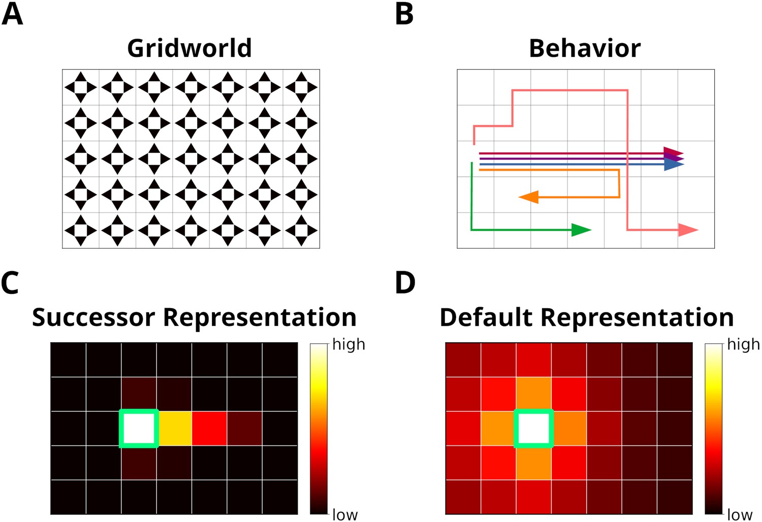
The grid world.

(A) An example of a simple grid world environment. An agent can transition between the different states, that is, squares in the grid, by moving in the four cardinal directions depicted by arrowheads. (B) Example trajectories of an agent moving in the grid world. (C) The successor representation (SR) for one state (green frame). Note that the SR depends on the agent’s actual behavior. (D) The default representation (DR) for the same state as in C. In contrast to the SR, the DR does not depend on the agent’s actual behavior and is equivalent to the SR given random behavior.

Here, we introduce a model of hippocampal replay which is driven by experience and environmental structure, and therefore does not require computing the hypothetical update that a stored experience would lead to, if it were reactivated. Especially during early learning, the sequences generated by our proposed mechanism are often the optimal ones according to Mattar and Daw, and our replay mechanism facilitates learning in a series of spatial navigation tasks that comes close to the performance of Mattar and Daw’s model. Furthermore, we show that a variety of hippocampal replay statistics emerges from the variables that drive our model. Hence, our model could be seen as an approximation of Mattar and Daw’s model that avoids the computation of hypothetical updates at a small cost to learning performance.

Results

Using structural knowledge and the statistics of experience to prioritize replay

We propose a model for the prioritization of experiences, which we call Spatial structure and Frequency-weighted Memory Access, or SFMA for short. The model was conceived with simplified grid world environments in mind (Figure 1A). Each node in the grid corresponds to an environmental state. During behavior a reinforcement learning agent transitions between nodes and stores these transitions as experience tuples $e_{t} = (s_{t}, a_{t}, r_{t}, s_{t + 1})$ . Here, s_t is the current state, a_t is the action executed by the agent, r_t is the reward or punishment received after transitioning, and $s_{t + 1}$ is the next state.

Reactivating stored experiences is viewed as analogous to the reactivation of place cells during replay events in the hippocampus. Assuming an experience e_t has just been reactivated, each stored experience $e$ is assigned a priority rating $R (e | e_{t})$ based on its strength $C (e)$ , its similarity $D (e | e_{t})$ to e_t and inhibition $I (e)$ applied to it (Figure 2A):

R (e | e_{t}) = C (e) D (e | e_{t}) [1 - I (e)]

Figure 2 with 3 supplements see all

Download asset Open asset

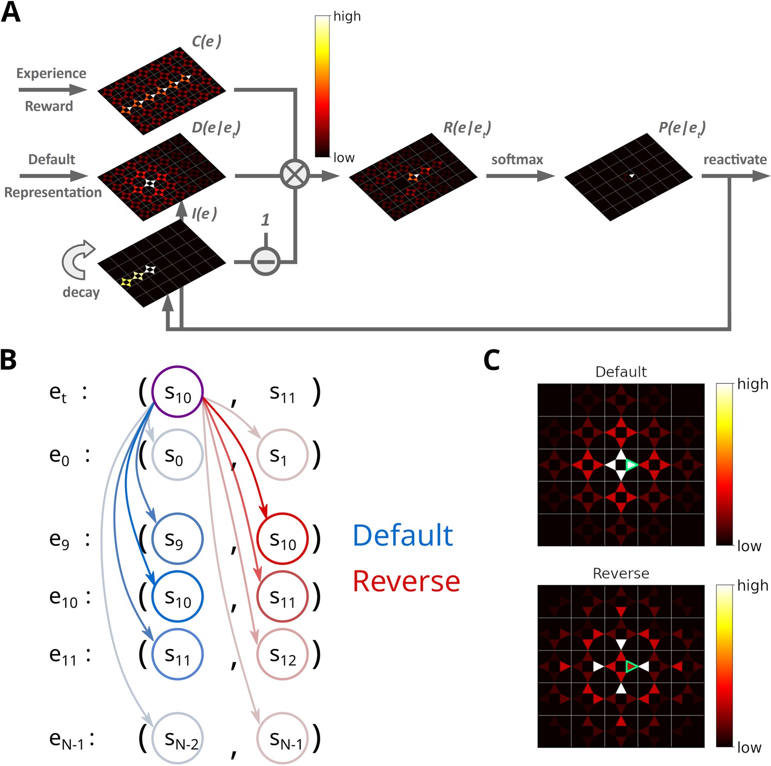
Illustration of the Spatial structure and Frequency-weighted Memory Access (SFMA) replay model.

(A) The interaction between the variables in our replay mechanism. Experience strength $C (e)$ , experience similarity $D (e | e_{t})$ and inhibition of return $I (e)$ are combined to form reactivation prioritization ratings. Reactivation probabilities are then derived from these ratings. (B) Experience tuples contain two states: the current state and next state. In the default mode, the current state of the currently reactivated experience (violet circle) is compared to the current states of all stored experiences (blue arrows) to compute the experience similarity $D (e | e_{t})$ . In the reverse mode, the current state of the currently reactivated experience is compared to the next state of all stored experiences (red arrows). (C) Example of the similarity of experiences to the currently reactivated experience (green arrow) in an open field for the default and reverse modes. Experience similarity is indicated by the colorbar. In the default mode, the most similar experiences are the current state or those nearby. In the reverse mode, the most similar experiences are those that lead to the current state.

The experience strength $C (e)$ is modulated by the frequency of experience and reward.

The similarity $D (e | e_{t})$ between e and e_t reflects the spatial distance between states, taking into account structural elements of the environment, such as walls and other obstacles. This rules out the use of Euclidean distances. A possible candidate would be the successor representation (SR) (Dayan, 1993). Given the current state state s_j, the SR represents as a vector the likelihood of visiting the other states s_i in the near future (Figure 1C). This likelihood is commonly referred to as the discounted future occupancy. Since states separated by a barrier are temporally more distant to each other than to those without a barrier, their expected occupancy is reduced more by discounting. However, the SR suffers from two disadvantages. First, the SR depends on the agent’s current behavior, i.e., the agent’s policy, which will distort the distance relationships between states unless that agent behaves randomly. Second, if the structure of the environment changes, the SR has to be relearned completely, and this may be complicated further by the first problem. These problems were recently addressed by Piray and Daw, 2021 in the form of the default representation (DR) (Figure 1D). Unlike the SR, the DR does not depend on the agent’s policy, but rather on a default policy, which is a uniform action policy, that is, random behavior, and the DR was shown to reflect the distance relationships between states even in the presence of barriers. Importantly, Piray and Daw, 2021 demonstrated that the DR can be efficiently updated if the environmental structure changes using a low-rank update matrix. We chose to base experience similarity on the DR due to its advantageous features.

Since experience tuples contain two states – the current state s_t and the next state $s_{t + 1}$ – we consider two ways of measuring the similarity between experiences. In the default mode, we compare the current states of two experiences (Figure 2B). In the reverse mode, the current state of the most recently reactivated experience is compared to the next states of the other experiences. We found that default and reverse modes tend to generate different kinds of sequences. Two more replay modes could be defined in our model, which we will not consider in this study. We explain this choice in the Discussion.

After an experience $e$ has been reactivated, inhibition $I (e)$ is applied to prevent the repeated reactivation of the same experience. Inhibition is applied to all experiences sharing the same starting state s_t, i.e., inhibition is set to $I (e) = 1$ , and decays in each time step by a factor of $0 < λ < 1$ . Inhibition values are maintained for one replay epoch and are reset when a new replay epoch is initiated.

The next experience to be reactivated is randomly chosen according to the activation probabilities $P (e | e_{t})$ , which are computed by applying a customized softmax function on $R (e | e_{t})$ (see Materials and methods). If the priority ratings for all experiences falls below a threshold $θ = 10^{- 6}$ replay is stopped. The definition of one replay epoch is summarized in Algorithm 1. Sequences of replay are produced by iteratively activating and inhibiting individual experiences. Together, experience strengths and experience similarities guide replay while inhibition promotes the propagation of sequences (Figure 2—figure supplement 1).

To initiate replay, we consider two cases: replay during awake resting states (online replay) is initiated at the agent’s current position, whereas replay during sleep (offline replay) is initiated with an experience randomly selected from memory based on the relative experience strengths. We chose different initialization schemes since awake replay has been reported to start predominantly at the animal’s current position (Davidson et al., 2009). However, there are also non-local sequences in awake replay (Karlsson and Frank, 2009; Gupta et al., 2010; Ólafsdóttir et al., 2017). Non-local replays are generated by our model in offline replay, albeit with a weaker bias for the current position (Figure 2—figure supplement 2A, B). To model awake replay, we could increase the bias in the random initialization by raising the experience strength for experiences associated with the current position (Figure 2—figure supplement 2C–F), while preserving some non-local replays. However, for simplicity we opted to simply initiate awake replay at the current location.

Algorithm 1. Spatial structure and Frequency-weighted Memory Access (SFMA)
Require: e_t (Replay initiated) 1: for t=1:N do 2: for experience $e$ do 3: Compute priority rating $R (e \| e_{t}) = C (e) D (e \| e_{t}) [1 - I (e)]$ . 4: end for 5: if $max R < θ$ then 6: Stop replay 7: end if : Compute reactivation probabilities $P (e \| e_{t})$ . 9: Choose next experience $e_{t + 1}$ to reactivate. 10: Reduce/decay inhibition for all stored experiences. 11: Inhibit experience $e_{t + 1}$ . 12: end for

Algorithm 1. Spatial structure and Frequency-weighted Memory Access (SFMA)

Require: e_t (Replay initiated)
1: for t=1:N do
2: for experience

e

do
3: Compute priority rating

R (e | e_{t}) = C (e) D (e | e_{t}) [1 - I (e)]

.
4: end for
5: if

max R < θ

then
6: Stop replay
7: end if
: Compute reactivation probabilities

P (e | e_{t})

.
9: Choose next experience

e_{t + 1}

to reactivate.
10: Reduce/decay inhibition for all stored experiences.
11: Inhibit experience

e_{t + 1}

.
12: end for

SFMA facilitates spatial learning

We begin by asking what benefit a replay mechanism such as implemented in SFMA might have for spatial learning. To do so, we set up three goal-directed navigation tasks of increasing difficulty: a linear track, a square open field, and a labyrinth maze (Figure 3A). Simulations were run for the default and reverse replay modes and compared to an agent trained without experience replay, an agent trained with random experience replay, and the state-of-the-art Prioritized Memory Access model (PMA) by Mattar and Daw, 2018.

Figure 3 with 4 supplements see all

Download asset Open asset

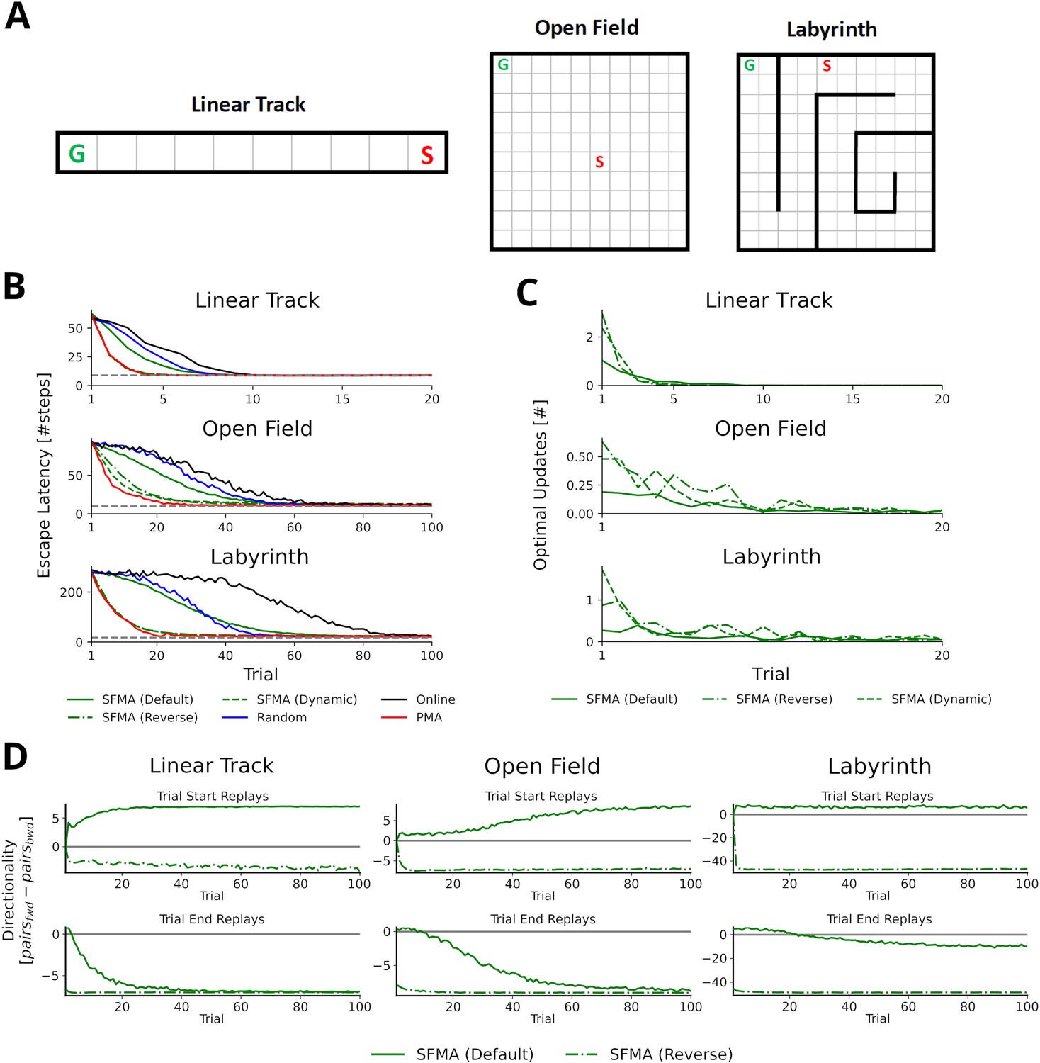
Statistics of replay has large impact on spatial learning.

(A) The three goal-directed navigation tasks that were used to test the effect of replay on learning: linear track, open field and maze. In each trial, the agent starts at a fixed starting location S and has to reach the fixed goal location G. (B) Performance for different agents measured as the escape latency over trials. Shown is the performance for an online agent without replay (black), an agent that was trained with random replay (blue), our SFMA model (green), and the Prioritized Memory Access model (PMA) by Mattar and Daw, 2018 (red). The results of our SFMA model are further subdivided by the replay modes: default (solid), reverse (dash-dotted), and dynamic (dashed). Where the dashed and dash-dotted green lines are not visible they are overlapped by the red solid line. (C) Reverse and dynamic replay modes produce more optimal replays while the default replay mode yields pessimistic replays. Shown is the number of optimal updates in the replays generated on each trial for different replay modes: default (solid), reverse (dash-dotted), and dynamic (dashed). Note, that in later trials there is a lack of optimal updates because the learned policy is close to the optimal one and any further updates have little utility. (D) Directionality of replay produced by the default (solid) and reverse (dash-dotted) modes in the three environments. The reverse replay mode produces replays with strong reverse directionality irrespective of when replay was initiated. In contrast, the default mode produces replays with a small preference for forward directionality. After sufficient experience with the environment the directionality of replays is predominantly forward for replays initiated at the start and predominantly reverse for replays initiated at the end of a trial.

Using the reverse mode, our model clearly outperformed the agents trained without replay and with random replay (Figure 3B). Importantly, performance was close to, even if slightly below, that of PMA. Learning performance of SFMA critically depends on the replay mode. The default mode yielded a performance that was much lower than the reverse mode and only slightly better than random replay. Considering its low performance, the default mode may appear undesirable, however, it is important for two reasons. First, it generates different types of sequences from the reverse mode (Figure 3D and Figure 3—figure supplement 1) and these sequences are more consistent with some experimental observations. While the reverse mode mostly generates reverse sequences in all situations, the default mode generates forward replay sequences at the beginning of trials and reverse sequences at the end of trials. This pattern of changing replay directions has been observed in experiments in familiar environments (Diba and Buzsáki, 2007). Also, as we will show below the default mode generates shortcut replays like those found by Gupta et al., 2010, whereas the reverse mode does not. Second, the recent discovery of so-called pessimistic replay, that is, replay of experiences which are not optimal from a reinforcement learning perspective, show that suboptimal replay sequences occur in human brains (Eldar et al., 2020) for a good reason (Antonov et al., 2022). Such suboptimal replays are better supported by the default mode (Figure 3C).

We therefore suggest that the reverse and default modes play distinct roles during the learning progress. Early in the learning session or following reward changes, when the environment is novel and TD errors are high, the reverse mode is preferentially used to acquire a successful behavior quickly (Figure 3—figure supplement 3). Indeed, in our simulations the reverse mode produces more updates that were optimal, that is, they improved the agent’s policy the most, than did the default mode (Figure 3C). The preponderance of reverse replay sequences during early learning is consistent with experimental observations in novel environments (Foster and Wilson, 2006) or after reward changes (Ambrose et al., 2016). Later in the learning session, when the environment has become familiar and TD errors are low, the default mode is preferentially used to make the learned behavior more robust. The default mode then accounts for interspersed reverse and forward replay sequences in familiar environments. We provide a more detailed rationale for the default mode in the Discussion. We call this strategy of switching between the reverse and default modes the dynamic mode of SFMA. Put simply, in the dynamic mode the probability of generating replay using the reverse mode increases with the TD errors accumulated since the last trial (for more details see Materials and methods). It yields a learning performance (Figure 3B) and number of optimal updates (Figure 3C) that are similar to the reverse mode.

In the following, we focus on the statistics of replay that SFMA generates in a range of different experimental settings.

Near-homogeneous exploration of an open environment explains random walk replays

We first investigated the replay statistics that our model produces in a simple environment without navigational goals similar to the experiment of Stella et al., 2019. To this end, we created a virtual square grid world environment of size 100 × 100 without rewards. For simplicity, we first set experience strengths to the same value, $C (e) = 1$ , to reflect homogeneous exploration of the environment. All replays were generated using the default mode since the environment was familiar to the animal in the experiments, but using the reverse mode did not affect the results (Figure 4—figure supplement 1).

With this setup the trajectories represented by the replayed experiences of the agent are visually similar to random walks (Figure 4A). The displacement distribution of replayed locations indicates that replay slowly diffuses from its starting location (Figure 4B and Figure 4—figure supplement 2). To analyze the trajectories more systematically, we used the Brownian Diffusion Analysis also used by Stella et al., 2019. In this analysis, a random walk is described by a power law relationship between the average distance between two replayed positions $Δ x$ and the time interval $Δ t$ , i.e., $Δ x = G Δ t^{α}$ with $α = 0.5$ . Indeed, the simulated replays exhibit a linear relationship in the log-log-plot indicating a power law between the two variables (Figure 4C) and the slope is close to the theoretical value for a random walk $α = 0.5$ . This result is robust across a large range of model parameters, the most relevant are the DR’s discount factor $γ_{D R}$ and inhibition decay $λ$ , and the range of values in our simulations, $α \in [0.467, 0.574]$ (Figure 4D), is a good match to the values reported by Stella et al., 2019. ( $α \in [0.45, 0.53]$ ). The values for the diffusion coefficient (Figure 4E), which relate to the reactivation speed, are similarly robust and only affected when the decay factor is close to zero. Hence, our model robustly reproduces the experimental findings.

Figure 4 with 5 supplements see all

Download asset Open asset

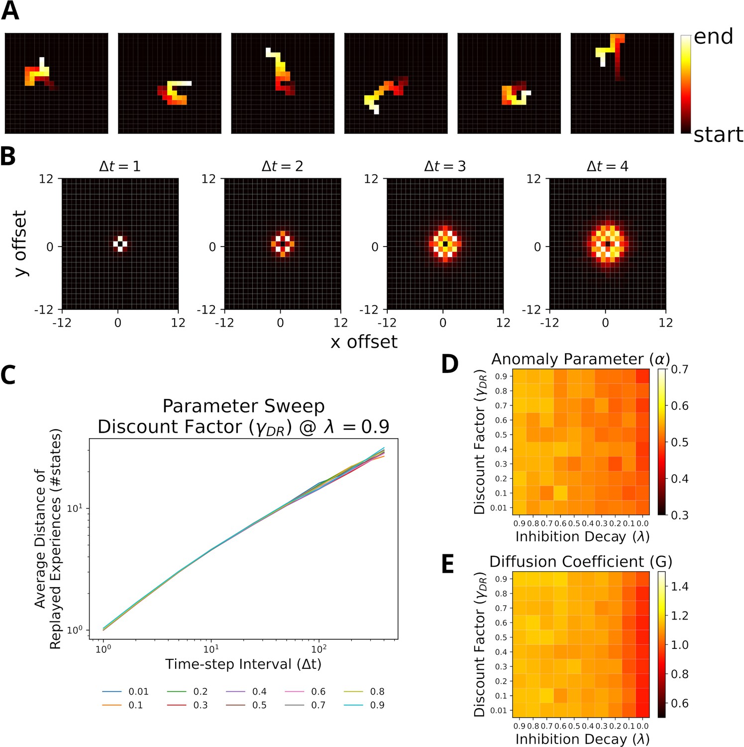
Replays resemble random walks across different parameter values for Default Representation (DR) discount factor and inhibition decay.

(A) Example replay sequences produced by our model. Reactivated locations are colored according to recency. (B) Displacement distributions for four time steps (generated with $β_{M} = 5$ ). (C) A linear relationship in the log-log plot between average distance of replayed experiences and time-step interval indicates a power-law. Lines correspond to different values of the DR’s discount factor $γ_{D R}$ as indicated by the legend. (D) The anomaly parameters (exponent $α$ of power law) for different parameter values of DR and inhibition decay. Faster decay of inhibition, which allows replay to return to the same location more quickly, yields anomaly parameters that more closely resemble a Brownian diffusion process, that is, closer to 0.5. (E) The diffusion coefficients for different parameter values of DR and inhibition decay. Slower decay of inhibition yields higher diffusion coefficients.

Since the results above were obtained assuming homogeneous exploration of the environment, we repeated our simulations with heterogeneous experience strengths (Figure 4—figure supplement 3B). While the relationships in the log-log-plot seems to slightly deviate from linear for very large time-step intervals, the statistics still largely resemble a random walk (Figure 4—figure supplement 3C). The range of values for $α \in [0.410, 0.539]$ still covers the experimental observations, albeit shifted toward smaller values.

Stella et al. further reported that the starting locations of replay were randomly distributed across the environment and replay exhibited no preferred direction. Our model reproduces similar results in the case of homogeneous experience strengths (Figure 4—figure supplement 4A, B) and heterogeneous experience strengths (Figure 4—figure supplement 4C, D). The results of our simulations suggest that replay resembling random walks can be accounted for given near-homogeneous exploration of an open-field environment. If exploration is non-homogeneous, the statistics of a random walk hold only for short to medium time-step intervals.

Stochasticity results in shortcut replays following stereotypical behavior

Gupta et al., 2010 provided further evidence that replay does not simply reactivate previously experienced sequences, by showing that replay sequences sometimes represent trajectories that animals were prevented from taking. These so-called shortcut sequences were synthesized from previously experienced trajectories. We constructed a simplified virtual version of the Gupta et al. experiment (Figure 5A) to test whether, and under which conditions, our proposed mechanism can produce shortcut replays. In the experiment, animals exhibited very stereotypical behavior, that is, they ran laps in one direction and were prevented from running back. Therefore, in our model the agent was forced to run one of three predefined patterns: right laps, alternating laps, and left laps (Figure 5B). This allowed us to focus on the effect of different specific behavioral statistics on replay. The virtual agent was made to run 20 trials in one session and replays were simulated after each trial.

Figure 5 with 3 supplements see all

Download asset Open asset

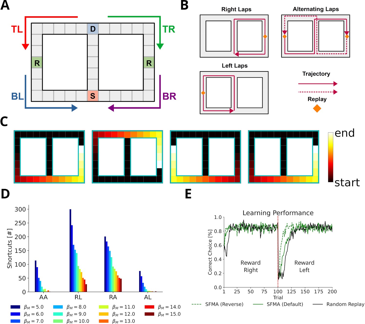
Replay of shortcuts results from stochastic selection of experiences and the difference in relative experience strengths.

(A) Simplified virtual version of the maze used by Gupta et al., 2010. The agent was provided with reward at specific locations on each lap (marked with an R). Trials started at bottom of the center corridor (marked with an S). At the decision point (marked with a D), the agent had to choose to turn left or right in our simulations. (B) Running patterns for the agent used to model different experimental conditions: left laps, right laps and alternating laps. Replays were recorded at the reward locations. (C) Examples of shortcut replays produced by our model. Reactivated locations are colored according to recency. (D) The number of shortcut replays pooled over trials for different running conditions and values of the inverse temperature $β_{M}$ . Conditions: alternating-alternating (AA), right-left (RL), right-alternating (RA), and alternating-left (AL). (E) Learning performance for different replay modes compared to random replay. The agent’s choice depended on the Q-values at the decision point. The agent was rewarded for turning right during the first 100 trials after which reward shifted to the left (red line marks the shift).

In the first 10 trials, the agents ran in one pattern, and in the next 10 trials, the agents used the same or a different pattern. To model Gupta et al.’s study, we ran simulations with the combinations right-left, right-alternating, and alternating-left. In addition, the combination alternating-alternating served as a baseline condition in which the left and right laps had roughly the same amount of experience throughout the simulation.

In this case, only the default mode could reproduce the experimental findings, while the reverse mode could not. The main cause lay within the large dissimilarity between the experiences at the decision point (D in Figure 5A) and the experiences to the left and right of it, which in turn drove prioritization values to zero.

We found that our model produces shortcut-like replays for each run pattern combination (Figure 5C and D). Shortcuts occurred in higher numbers for right-left and right-alternating combinations, and mainly in the last 10 trials, in trials when the agent was running a left lap, that is, every trial for right-left and every other trial for right-alternating (Figure 5—figure supplement 1). Across the whole running session, for alternating-alternating and alternating-left combinations a lower number of shortcuts occurred. This difference between combinations results from the balance of experience strengths associated with either of the laps and with the center piece. For right-alternating and right-left combinations the experience strengths associated with right lap and center piece were similar and therefore replay, when initiated at the left lap’s reward location, was not biased to reactivate experiences along the center piece. The number of shortcut replays then decreased as the experience strengths associated with the center piece increased relative to those associated with either of the laps. Since for alternating-left and alternating-alternating combinations the experience strengths associated with the center piece already were higher relative to those associated with the laps an overall low but constant number of shortcut replays was produced.

Across all conditions the number of shortcut replays decreased with increasing inverse temperature $β_{M}$ , which transforms priority ratings to reactivation probabilities. The larger $β_{M}$ , the more deterministic replay becomes. This result therefore suggests that shortcut replay is driven by stochasticity in the prioritization process (Figure 5D and Figure 5—figure supplement 1) and differences in relative experience strengths (Figure 5—figure supplement 2) of the maze’s center piece and arms. These differences are in turn induced by the specific behavioral statistics.

Finally, we wanted to know if replay facilitates learning in this task. Since the agent cannot remember, which lap it ran in a previous trial, it would not be able to learn with alternating rewarded locations. Therefore, we chose the right-left condition as the learning task. To deal with problematic behavior of the simple RL agents mentioned above we adjusted our simulation to only consider the action selected at the decision point and let the agent run straight otherwise. We ran simulations in default and reverse mode. An agent trained with random experience replay was used as the baseline. All agents solved the task and successfully learned the new goal location after the rewarded locations changed from right to left (Figure 5E). Both default and reverse mode yielded faster learning than random experience replay. However, there was no large difference between the replay modes during the first half. These small differences in learning performance suggest that replaying strictly in reverse mode may not be necessary in tasks with stereotypical behavior since the resulting experience strengths would naturally guide replays in forward or reverse depending on where replay started (Figure 5—figure supplement 3).

Dynamic structural modulation allows replay to adapt to environmental changes

Recently, Widloski and Foster, 2022 reported that hippocampal replay dynamically adapts to daily changes in the structure of the environment. We argue that this type of replay can be accounted for by representing the environmental structure dynamically with the default representation (DR) (Piray and Daw, 2021). While the SR (Dayan, 1993) could also be used to represent the environment’s structure, it cannot be updated efficiently in the face of structural changes and depends on the agent’s policy. The DR does not suffer from these problems. Specifically, we employed the DR by separating the spatial representation into open 2D space and information about environmental barriers. Barrier information was provided when the environment changed (see Methods).

To test whether our proposed replay mechanism can adapt to changes of the environment’s structure, we simulated replays in three distinct consecutive environments (Figure 6A) and evaluated the occurrence of replay crossing environmental barriers. All replays were generated using the default mode, but using the reverse mode did not affect these results (Figure 6—figure supplement 1). Our proposed replay mechanism successfully adapts to changes in the environment’s structure as illustrated by replays diffusing along barriers in the reactivation maps (Figure 6A) and shown by the absence of invalid transitions (Figure 6C). In contrast, when experience similarity is based on the Euclidean distance between locations, replay does not conform or adapt to the changing environmental structure (Figure 6B and C).

Figure 6 with 1 supplement see all

Download asset Open asset

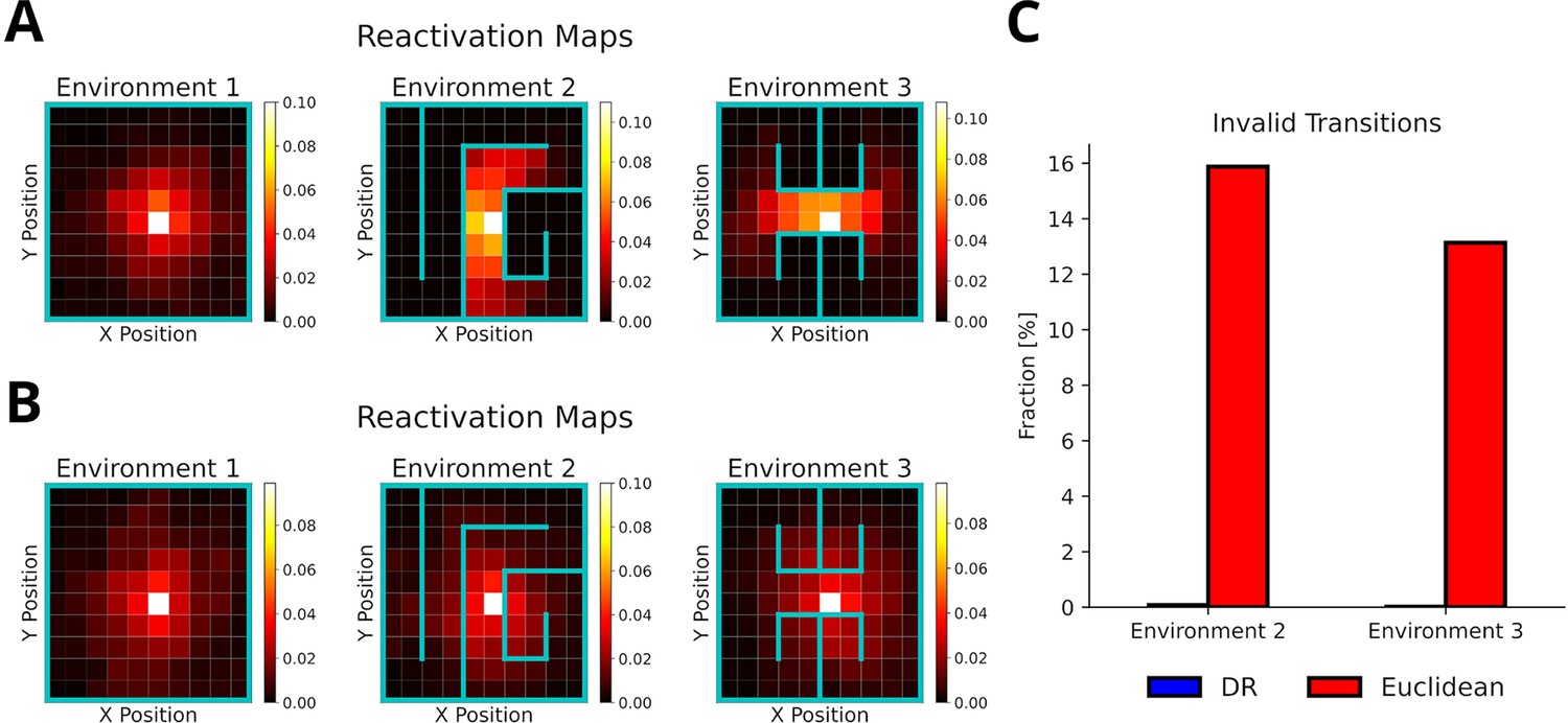
The default representation (DR) allows replay to adapt to environmental changes.

(A) Reactivation maps, that is, the fraction of state reactivations, for all replays recorded in three environments while the agent is located at the white square. Experience similarity is based on the DR with a discount factor $γ_{D R} = 0.1$ . The colorbar indicates the fraction of reactivations. Note that replay obeys the current environmental boundaries. (B) Same as in A, but experience similarity is based on the Euclidean distance between states. Note that replay ignores the boundaries. (C) The fraction of invalid transitions during replay in different environments for the DR (blue) and Euclidean distance (red). While replay can adapt to environmental changes when using the DR, it does not when experience similarity is based on the Euclidean distance.

Preplay of unvisited locations requires structural modulation and visual exploration

Ólafsdóttir et al., 2015 reported the preplay of trajectories through a part of a T-maze that the animal could see, but not physically explore, and that contained a visible reward. Our model can provide an intuitive explanation for the reported phenomenon. First, the use of DR explains, in principle, why the preplay of unvisited locations is possible. The DR allows for the representation of the environment’s structure provided it is observable. Still, these experiences would have zero experience strength in our model and therefore would not be reactivated. However, during the reward cueing phase, the animals were reported to have paid attention to the reward cue. We view this as a form of visual exploration that increases the strength of experiences along the attended arm and updates the reward information related to the experiences.

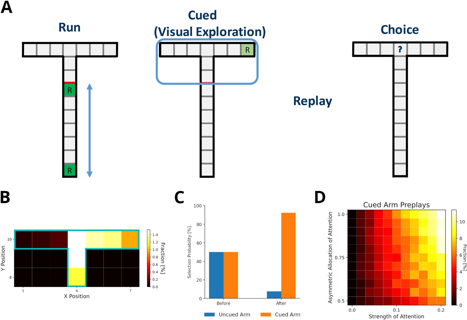
We set up a virtual version of the Ólafsdóttir et al., 2017 task (Figure 7A) in which the agent first runs up and down the maze stem ten times with rewards provided at each end of the stem (run phase). In the cued phase, we increased experience strengths of the blocked arms by a small amount relative to actual exploration (attention strength), which was larger for the cued than the uncued arm (asymmetric allocation of attention). Then experiences were preplayed. Template matching was used to detect the preplay of cued and uncued arms, and replay of the stem. All preplays were generated using the default mode, but results were similar when using the reverse mode (Figure 7—figure supplement 1). We found that our model indeed produces preplays of the cued arm and only rarely of the uncued arm (Figure 7B). As expected, the attention strength as well as the asymmetric allocation of attention are key to produce preplays (Figure 7D). The higher the value of these two parameters, the more often the cued arm is preplayed.

Figure 7 with 1 supplement see all

Download asset Open asset

Preplay of cued, but unvisited, locations can be explained by visual exploration.

(A) Schematic of the simplified virtual maze and task design used to model study by Ólafsdóttir et al., 2015. First, in an initial run phase, the agent ran up and down the stem of the maze. Second, in the following visual exploration phase, the agent visually explores a cued part of the maze and increases the strength of the associated experiences. Third, experiences are reactivated according to their priority scores. Fourth, agents are given access to the entire T-maze. The fraction of choosing the two arms in the test phase are compared. (B) Fractions of reactivated arm locations. Experiences associated with the cued arm (right) are preferentially reactivated. (C) The fractions of choosing either arm before and after training the agent with preplay. Before preplay the agent shows no preference for one arm over the other. After preplay, the agent preferentially selects the cued arm over the uncued arm. (D) The percentage of cued-arm preplay (out of all arm preplays and stem replays) for different amounts of attention paid to the cued arm vs. the uncued arm (asymmetric allocation of attention) and experience strength increase relative to actual exploration (attention strength).

Furthermore, Ólafsdóttir et al., 2017 reported that animals preferred the cued arm when the barrier blocking the arms was removed and they were given physical access to the maze. Our model shows the same preference for the cued arm after training an agent with simulated replays and testing it in the T-maze (Figure 7C).

Reward modulation of experience strength leads to over-representation of rewarded locations

Replay is known to over-represent rewarded locations (Singer and Frank, 2009; Pfeiffer and Foster, 2013). This might be accounted for in our model, since the experience strength $C (e)$ is modulated not only by the frequency of experience but also by the frequency of reward. However, it is not intuitively clear how their relative contribution affect the statistics of replay. We therefore tested different values for reward modulation, that is, the increase of experience strength due to reward, in goal-directed navigation tasks in open field and T-maze environments. The default value used in other simulations was one. These simuluations were compared to those with a reward modulation of ten. Note, in our model changing the reward modulation is equivalent to changing the magnitude of reward.

Training lasted for 100 trials. Online replays were generated at the beginning and end of each trial. Additionally, offline replays were also generated after each trial. However, only online replays generated at the end of a trial were used to train the agent. All replays were generated using the default mode.

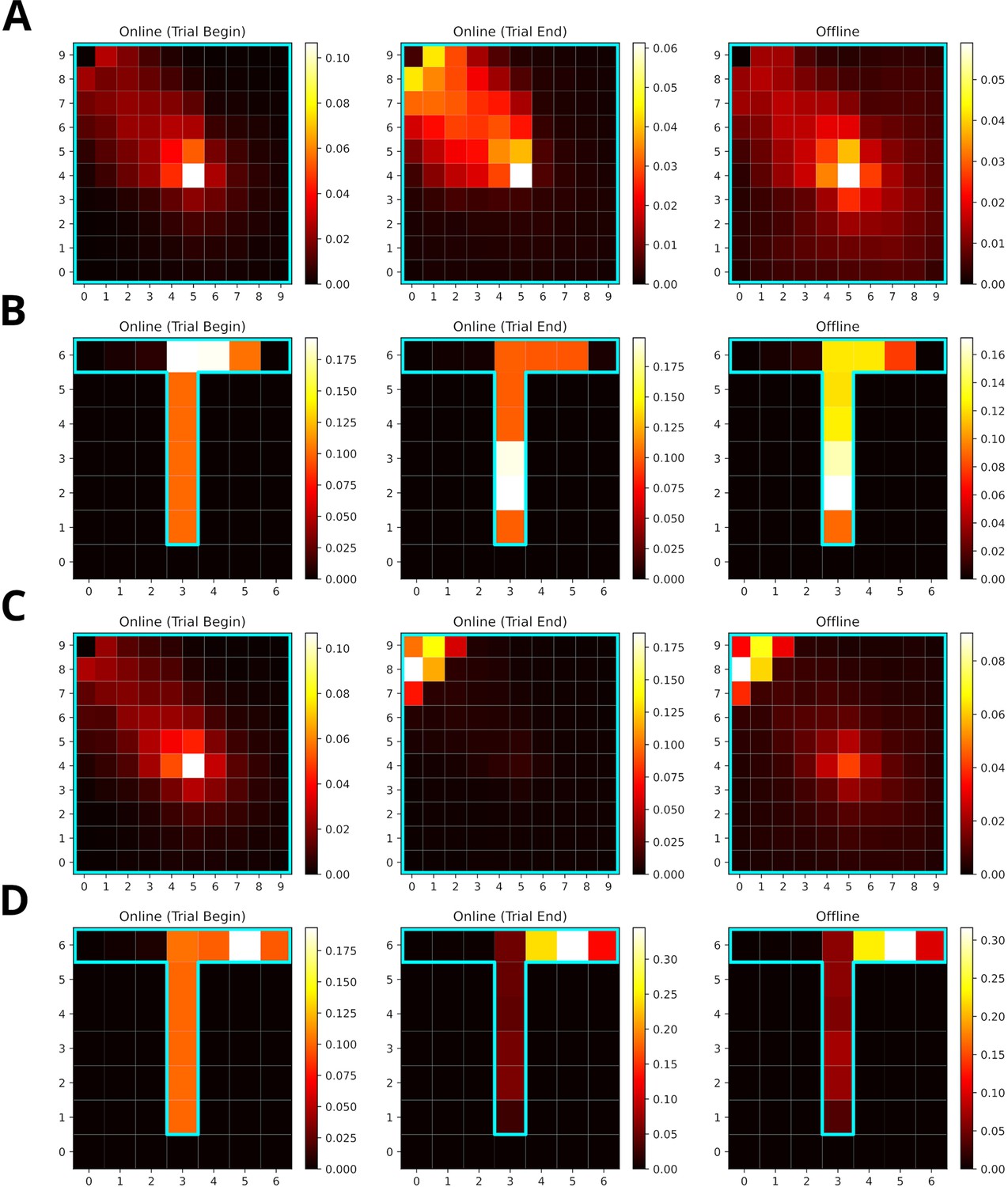
When the frequency of experience and reward modulate experience strength equally, replays mainly represent locations along the path leading to the rewarded location (Figure 8A and B). Replays in the open-field environment over-represent the starting location. The rewarded location shows stronger over-representation for online replays occurring at the end of trials partly due to initialization bias at the goal location. In the T-maze, these effects are less pronounced due to replay being constrained by the maze’s structure. Increasing the reward modulation to ten, drives replays to over-represent the rewarded location (Figure 8C and D). For online replays at the beginning of trials, this effect is not apparent due to the initialization bias at the starting location. For online replays at the end of trials and offline replay, the representation of the path leading to the rewarded location is heavily reduced and that of the goal location is enhanced.

Figure 8

Download asset Open asset

Increasing the reward modulation of experience strengths leads to an over-representation of rewarded locations in replays.

(A) Reactivation maps for online replays generated in an open field environment at trial begin (left) and end (middle) as well as for offline replays (right). Reward modulation was one. Replay tends to over-represent the path leading to the reward location. The starting location is strongly over-represented for all replay conditions, while the the reward location is mainly over-represented for trial end replays. (B) Same as A, but in a T-maze. (C) Same as A, but due to a higher reward modulation of ten the rewarded location is strongly over-represented in replay. (D) Same as C, but in a T-maze.

To summarize, SFMA can account for the over-representation of rewarded locations reported in the literature and this over-representation depends on the balance of modulation due to experience and reward.

Replay enters aversive locations given previous experience, driving the learning of avoidance

Replay was found to not only form reward-directed sequences, but also, rather counter-intuitively, to enter locations associated with aversive experiences (Wu et al., 2017). The specific location and amount of replay reported by Wu et al., 2017 is not within the scope of our model. Nonetheless, SFMA can give a simple account for why replay would enter aversive locations. In their study, the animals had substantial experience with the whole environment, which consisted of a dark and light zone, over three phases (Run 1, Run 2, and Pre) before shock was introduced in the dark zone. Importantly, the animals initially displayed a strong bias for the dark zone.

For our simulation, we used a 20-states-long linear track where the left and right half represented dark and light zones, respectively. The left most two states represented the shock zone. We modeled the initial three phases by having an agent run 30 laps on the linear track environment and multiplied the experience strengths associated with the dark and light zones with the occupancy reported by Wu et al., 2017. The remainder of the simulation consisted of a single shock trial in which the agent entered the shock zone and received shock of magnitude one, and nine trials in which the agent ran laps in the light zone. Twenty replays of length ten were generated after receiving the shock. While running laps in the light zone, replays were generated when the agent stopped in front of the dark zone. The generated replays preferentially entered the dark zone and reached the shock zone (Figure 9A). This is due to the agent’s previous experience in the dark zone, which was over-represented relative to the light zone.

Figure 9

Download asset Open asset

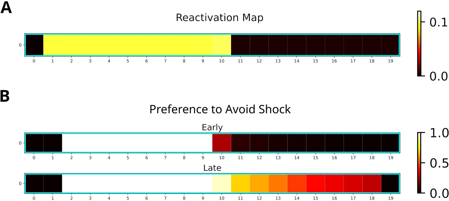
Replay will enter aversive zones given previous experience.

(A) The reactivation map indicates that the dark zone (left half), which contains the shock zone, was preferentially replayed even after the shock administered and the agent stopped in the middle. (B) Probability of the Q-function pointing away from the shock zone for each state. After the first five trials (Early), avoidance is apparent only for states in the dark zone (excluding the shock zone itself). In the following five trials (Late), the preference for avoidance is propagated to the light zone (right half).

Additionally, we investigated the effect of the generated replays on behavior by training the agent and analyzing the policy. The learned policy preferentially points away from the shock zone (Figure 9B), indicating that the agent learned to avoid the shock zone. Avoidance is stronger following more replay and spreads to the light zone (Figure 9B, bottom map). Our simulations suggest that previous experience is sufficient for replay to produce sequences that extend to aversive locations and that these sequences could further facilitate the learning of avoidance behavior.

Discussion

We introduced a replay mechanism (SFMA) that accounts for a variety of different replay statistics reported in the literature. The core aspect of SFMA is the prioritization of experiences according to the frequency at which they occur, the likelihood with which they are rewarded, and the structure of the environment. Furthermore, reactivated experiences are inhibited in the prioritization process to drive the generation of sequential activations. The statistics of these sequences depend on whether SFMA operates in the default or reverse mode. Surprisingly, despite these differences both modes are consistent with diverse experimental results – with the notable exception of shortcut replays, which arise only in the default mode. However, the two modes have very different impact on spatial learning, which is much faster when using the reverse mode. In the following we discuss some details of our modeling assumptions and results.

The components of the spatial structure and frequency-weighted memory access (SFMA) model

The prioritization of experiences during replay is well supported by experimental evidence. Behavioral data suggests that animals use spatial representations to quickly adapt to changes in the environment (de Cothi et al., 2020). Structural modulation of hippocampal replay is reported in the literature (Wu and Foster, 2014; Ólafsdóttir et al., 2015; Widloski and Foster, 2022). The hippocampus and related structures, for example, entorhinal cortex (EC), are commonly known for containing cells that selectively fire for spatial features (O’Keefe and Dostrovsky, 1971; Hafting et al., 2005; O’Keefe and Burgess, 1996). We chose to represent the environment’s structure with the default representation (DR) (Piray and Daw, 2021), which is a special case of the successor representation (Dayan, 1993). The latter has been proposed to explain firing properties of place and grid cells (Stachenfeld et al., 2017), and the DR gives an account for boundary cells in EC (Piray and Daw, 2021). Furthermore, we separated the representation of space into a general representation of 2D space and information about environmental barriers. It has been proposed that the hippocampal place cell code is formed by combining a learned representation of the task structure (e.g. space) with sensory information (Whittington et al., 2020). We propose that SFMA’s similarity term is likely implemented through spatial representations found in the hippocampus and EC. Namely, place cell activity could provide the hippocampus access to the experience similarities or at least an estimate of them without the need for taxing computation.

The frequency of experience (Kudrimoti et al., 1999; O’Neill et al., 2008; Gillespie et al., 2021) as well as reward Pfeiffer and Foster, 2013 have been shown to influence the content of replay. The experience strength term of SFMA is consistent with these experimental findings. Experience has also been incorporated in other models. For instance, the Mattar and Daw, 2018 model uses the Successor Representation which depends on the agent’s previous behavior. However, integrating the frequency of an experience $f_{E} (e)$ and the frequency/size of reward $f_{R} (e)$ into one variable, the experience strength, as SFMA does, renders replay less flexible and could negatively affect learning. For instance, extreme over-representation of the rewarded locations may slow down the propagation of reward information to locations far away from them. More flexibility could be introduced by separating the two parameters more clearly and computing experience strength as a weighted average $C (e) = w_{E} f_{E} (e) + w_{R} f_{R} (e)$ . The weighting could then be flexibly adjusted depending on the situation. A potential way for a biological network to implement experience strength could be to increase the overall excitability of place cells after experience (Pavlides and Winson, 1989) and especially when reward was encountered (Singer and Frank, 2009).

Inhibition of return could easily be implemented via local inhibitory recurrent connections and experience strength through strengthening of connections between cell assemblies. While the main purpose of inhibition is that it enables the generation of sequences, it can be also viewed as a way of shifting priorities from experiences that were already used during learning to other experiences and, hence, ensuring the propagation of reward information. An interesting question pertains to whether a similar inhibition mechanism is utilized in the hippocampus. It was shown in modeling studies that the generation of sequences in a network does not strictly require inhibition (Bayati et al., 2015). However, forms of inhibition have been used to account for replay as well as preplay sequences in biologically plausible models (Chenkov et al., 2017; Azizi et al., 2013). We propose that the existence of inhibition implemented in our model could be tested by measuring the excitability of place cells following their reactivation during replay events.

In summary, the variables that SFMA uses for prioritization could be realized in an efficient manner by the hippocampus.

The role of different replay modes in our model

While the default mode accounts for all varieties of replay statistics considered, it performs considerably worse during learning than the reverse mode since it does not produce reverse sequences as reliably. Reverse sequences are important for learning because they can propagate rewards information back to preceding actions that led to the reward (Foster and Wilson, 2006).

To benefit from the advantages of both replay modes, we propose that they could play different roles during learning. There is support in the literature for this view. Foster and Wilson, 2006 found that reverse replay can occur after even a single experience, which is predominantly generated by the reverse mode. Furthermore, the frequency of reverse replay has been observed to increase in response to positive reward changes (Ambrose et al., 2016). Hence, the reverse mode might be used preferentially when the situation requires learning and the switch to the reverse mode may be triggered by neurons encoding reward prediction error (Schultz et al., 1997). By contrast, Wikenheiser and Redish, 2013 reported both forward and reverse replay sequences during awake resting phases occurring in roughly equal proportions (for a whole session). In a familiar environment, Diba and Buzsáki, 2007 found that replay sequences in forward order at the beginning of a trial prior to running on a linear track and in reverse order at the end of a trial after running. These results are more consistent with the default mode and more balanced replay direction in familiar environments.

What could the function of the default mode be, if it does not speed up learning much compared to random replay? A possibility could be a supportive function in the RL process. For instance, in the context of deep RL it is well known that multi-layer networks trained with sequences suffer from learning instabilities (Mnih et al., 2015). These instabilities are addressed by randomly replaying experiences to break the strong temporal correlations between sequential experiences. While not completely random, the default mode is more likely to break proper reverse and forward sequences. Another possible function that could be implemented by the default mode is the reactivation of experiences which otherwise would not (or only rarely) be reactivated in the reverse mode. Recent findings of pessimistic replay, i.e., the replay of sub-optimal experiences, in humans (Eldar et al., 2020) supports this view. Interestingly, follow-up modeling work (Antonov et al., 2022) suggests that optimal replay occurs predominantly during initial trials and then switches to pessimistic replay. However, this switch is dependent on the utility of experiences (Mattar and Daw, 2018). The default mode could be viewed as enabling these pessimistic replays, and the switch from optimal to pessimistic replay corresponds to the dynamic mode in our model.

Alternatively, the default mode might not be directly related to RL, but serve a different function altogether. For instance, the sequences generated in the default mode might be important for maintaining synaptic connections which otherwise would not be maintained due to the specific distribution of reverse replays (Hebb, 1949; Caporale and Dan, 2008). Another function often attributed to hippocampal replay is that of planning (Diba and Buzsáki, 2007; Buckner, 2010; Buhry et al., 2011) by simulating possible future trajectories to inform subsequent behavior. The default mode could, in principle, support this function. In contrast, since the reverse mode almost exclusively produces reverse sequences, it could not support the prospective sequences needed for planning.

Two further replay modes can be defined in our model, which we did not consider in our study. An attractor mode, which compares the next state of experience e_t with the next state of all stored experiences e. Hence, this mode looks for experiences that end in the same state, so that neighboring experiences are activated in a ring-like fashion (Figure 2—figure supplement 3). Since we are not aware of any experimental studies reporting such ring-like replay, we did not consider this mode in our study. Another possible replay mode, is the forward mode, which compares the next state of experience e_t with the current state of all stored experiences e. The forward mode exclusively produces forward replays, which are not efficient for learning, but could very well efficiently support planning. The latter is, however, outside the scope of the current study. Furthermore, the forward mode is not as flexible as the default mode in generating transitions between states that were never (or rarely) experienced, and replaying such transitions could be useful for discovering novel solutions.

How might default and reverse modes be implemented by a biological network? The default mode could be implemented as an attractor network where each experience’s current state is stored as an attractor. The currently reactivated experience/state would be represented by a bump of activity in the network. Due to self-inhibition the bump would be driven to leave the current attractor state and move to a close-by, i.e., similar, one.

The reverse mode requires two attractor networks, net0 and net1, to store the current and subsequent states of each experience, respectively. They are assumed to use the identical representations. In addition, the state transitions $(s_{t}, s_{t + 1})$ are encoded in the weight matrix w₁₀ between net1 and net0. An experienced transition is stored by learning a connection from $s_{t + 1}$ in net1 to s_t in net0. When an experience is replayed in the reverse mode, the pattern representing $s_{t + 1}$ is activated in net1, which in turn excites the state s_t in net0. The weights w₀₁ from net0 to net1 are assumed to be one-to-one connections, so that the activity pattern in net0 activates the most similar pattern in net1, equivalent to our algorithm finding, in all experiences, the next state that is closest to the current state of the reactivated experience. And the process of reactivating experiences iterates from here, thereby resulting in reverse replay.

Since the reverse replay has to perform one more computational step than the default mode, that is, the transition from $s_{t + 1}$ to s_t, this would suggest that generating sequences in the reverse mode is slower, which is consistent with experimental observations (Liu et al., 2021).

Current limitations of SFMA

SFMA accounts for the statistics of replay sequences and generates sequences that drive learning efficiently. However, in its current version, it addresses neither when replay events should occur nor the overall amount of replay. This limitation also extends to other similar models that implement a fixed number of update steps (Mattar and Daw, 2018) or initiate replay at predefined points in time (Khamassi and Girard, 2020). This limitation leaves certain aspects of a variety of experimental findings outside of the scope of our model. For instance, Cheng and Frank, 2008 reported that replay decreases across sessions as the animals became more familiar with their environment, and Ambrose et al., 2016 found that the number of SWRs and replay increases or decreases with changing reward magnitude. Nonetheless, Mattar and Daw, 2018 argue that their model accounts for both these findings by focusing on the number of ‘significant’ replays produced by their model, which decreases with familiarity with the environment and when reward decreases, and increases when reward increases. For SFMA, a similar effect w.r.t to the familiarity occurs in the default mode: As familiarity with the environment increases and the agent’s policy stabilizes, longer forward and reverse sequences are produced at the start and end of trials (Figure 3—figure supplement 4). Given the fixed number of replay steps, this results in a lower number sequences.

In PMA, the amount of reverse replay is driven by the gain term of the prioritization scheme. This is because gain is the main driver of reverse sequences and gain increases for positive reward changes. However, if gain is low, replay is dominated by the need term instead thereby resulting in the absence of reverse replays. While SFMA cannot account for the overall change in amount of replay due to changes in reward it can explain the shift in the statistics of occurring replay with the dynamic mode. The dynamic mode determines whether to produce replay using the reverse mode, which predominantly generates reverse sequences, given the recent history of prediction errors. Indeed, in open field and T-maze environments, we find that reward changes results in replays being generated in the reverse mode more often (Figure 3—figure supplement 3). However, this does not match the experimental findings which show a decrease of reverse replay for negative reward changes (Ambrose et al., 2016). Unlike PMA, SFMA therefore cannot account for the differential effects of reward change in its current form.

Recent findings show that replay can be influenced by motivational shifts (Carey et al., 2019). SFMA and other similar models may not be suitable to account for these findings, since they do not differentiate between different types of reward and do not consider different behavioral states like hunger or thirst. Changes in behavior due to motivational shifts could be explained by the learning of separate Q-functions for different sources of reward and then choosing the Q-function which corresponds to the current motivation. In Carey et al., 2019 two reward sources, that is, food and water, were available to the animals. When one was restricted behavior shifted towards it, but replay shifted toward the unrestricted one. While SFMA may produce replays representing the unrestricted reward source, it would not be able to account for the observed shifts in replay content due to shifts in motivation. SFMA could potentially account for the shift in replay content by including the recency of experience during prioritization. If more remote experiences have their priority increased, the content of replay could shift in a similar way to the one reported. Another account for the content of replay shifting to represent the unrestricted reward source is given by the model by Antonov et al., 2022. In their model, which is partly based on PMA, the agent’s Q-function is subjected to forgetting, which eventually leads the utility of transitions not updated recently to increase. Since during behavior the restricted reward source is preferentially visited, the unrestricted reward source would be more affected by forgetting. This would lead to replay representing the unrestricted reward source more often. Both potential mechanisms would produce the shift of replay content as a result of the behavioral history rather than due to motivational shift directly.

Gillespie et al., 2021 reported that awake replay preferentially represented previously rewarded goal locations rather than the current one. Since experience strength is modulated by both reward and previous behavior this finding could potentially be accounted for by our model. However, the experiment also found that locations that have not been visited recently are represented more often. This effect of behavioral recency can currently not be accounted for by SFMA. The two potential mechanisms discussed in the above paragraph could enable SFMA to also account for the effect of behavioral recency.

Related work

The work closest to ours is the state-of-the-art PMA model by Mattar and Daw, 2018. It proposes that replay prioritizes experiences according to their utility, which in turn is defined as the product of gain and need. Gain represents the policy improvement that would result hypothetically if an experience were reactivated and need represents the expected future occupancy of the experience’s current state. As mentioned in the introduction, it is not clear how a biological neural network could compute the utilities for stored experiences. Our model circumvents this problem by basing the probability of reactivation on behavioral and environmental variables and offers a potential account for how the utility of experiences could be approximated.

Furthermore, the implementation of PMA contains a few oddities. Because utility is defined as a product of gain and need, the gain must have a nonzero value to prevent all-zero utility values. This is achieved by applying a (small) minimum gain value. A problem arises for the special $n$ -step update, which updates the Q-function for all n states along the replay trajectory, considered by their model for which gain is summed over $n$ steps and which is the main driver of forward sequences (especially, for offline replay). The minimum gain value is applied before summation, so that the gain artificially increases with sequence length. Furthermore, Mattar & Daw state that ‘EVB ties are broken in favor of shorter sequences’, where EVB stands for ‘expected value of backup’, that is, the utility. By contrast, due to their implementation, longer sequences are always favored in the case when gain is zero for all experiences, which can occur when the environment does not contain reward or the environment is highly familiar. This artifact could be avoided by applying the minimum value only once after the summation of gain values. In our hands, this reduces the model’s ability to produce sequences during offline replay, because the utility is dominated by the gain term (Figure 4—figure supplement 5).

A different view of hippocampal replay was presented by Khamassi and Girard, 2020. They argue that replay can be viewed as a form of bidirectional search in which learning is facilitated by alternating between phases of prioritized sweeping (Moore and Atkeson, 1993), which prioritizes experiences according to how their reactivation affects behavior, and trajectory sampling (Sutton and Barto, 2018), which explores potential routes by simulating trajectories through the environment. In simulations, they show that bidirectional search performs better than prioritized sweeping and trajectory sampling alone. Importantly, they also were able to reproduce the occurrence of shortcut replays. Their model is, in principle, able to generate random walk replays due to the fact that, in the absence of reward, replay would be dominated by the trajectory sampling phase under a uniform action policy. However, their model does not give an account for how replay could adapt to environmental changes.

McNamee et al., 2021 proposed a generative model of replay which adapts replay statistics depending on the cognitive function that it supports. Unlike the models discussed above, this model focuses on states, that is, locations, reactivated and ignores the combination of state and action. Their model produces random walks and they show that these replay statistics facilitate the learning of a successor representation of the environment. However, this model lacks a proper account for why replay should be able to quickly adapt to changes in the environment, and assumes a generator for (random) sequences which is handcrafted for each simulation. Furthermore, their model does not seem to allow for differentiating forward from reverse sequences.

Conclusion

Our model gives a biologically plausible account of how the hippocampus could prioritize replay and produce a variety of different replay statistics, and fits well with contemporary views on replay. Furthermore and most importantly, the replay mechanism facilitates learning in goal-directed tasks, and performs close to the current state-of-the-art model without relying on computations of hypothetical network updates.

Materials and methods

Reinforcement learning

Request a detailed protocol

For our computational study we relied on reinforcement learning (RL) (Sutton and Barto, 2018) which makes it possible to learn optimized sequences of choices based on sparse rewards. In RL, an agent interacts with an environment and tries to maximize the expected cumulative reward (Sutton and Barto, 2018):

R = E [\sum_{t} γ^{t} r_{t}],

where $γ$ is the so-called discount factor that weighs the importance of rewards that will be received in the future relative to immediate ones, and r_t is a real-valued reward received at time $t$ . The RL agent must learn to choose those actions that maximize the expected cumulative reward, the so-called optimal policy, through interactions with its environment. These interactions are generally formalized as experience tuples $e_{t} = (s_{t}, a_{t}, r_{t}, s_{t + 1})$ , where s_t and $s_{t + 1}$ denote the current state and next state, respectively. The action taken by the agent in state s_t is represented by a_t and the scalar reward received is represented by r_t. The critical problem in RL is crediting the right choices leading to a reward that was received only (much) later.

A popular algorithm that solves this learning problem is Q-learning (Watkins, 1989) which uses a state-action value function $Q (s, a)$ , also called the Q-function, to represent the cumulative future reward expected for taking action $a$ in state $s$ . The Q-function is updated from experiences in each time step $t$ by:

Q (s_{t}, a_{t}) \leftarrow Q (s_{t}, a_{t}) + η [r_{t} + γ \max_{a} Q (s_{t + 1}, a) - Q (s_{t}, a_{t})]

Here, $η$ denotes the learning rate. For all simulations the learning rate was set to $η = 0.9$ . The term in brackets is known as the temporal difference error, and represents by how much the last action and potentially collected reward has changed the expected discounted future reward associated with the state. RL generally requires many interactions with the environment, which results in slow learning. To address this problem Lin, 1992 introduced experience replay, where interactions with the environment are stored as experiences e_t and reactivated for updating the Q-function later. In its simplest form, experience replay samples stored experiences uniformly at random. Learning from replay can be further improved by prioritizing experiences to be replayed (Sutton and Barto, 2018; Schaul et al., 2016).

Spatial structure and frequency-weighted memory access (SFMA)

Request a detailed protocol

For our simulations, we employed the Dyna-Q architecture in combination with grid world environments in a similar fashion to Mattar and Daw, 2018. We view the reactivation of specific experiences as analogous to the reactivation of place cells in the hippocampus during awake and sleeping resting states. Like the original Dyna-Q architecture, our model stored experiences for all environmental transitions in a memory module. However, we stored additional variables for later prioritization of experiences during replay: The experience strength $C (e_{i})$ , the experience similarity $D (e_{i} | e_{j})$ and inhibition of return $I (e_{i})$ . The experience strength is a count of how often a certain environmental transition was experienced. Following an experienced transition e_i the experience strength was updated as follows:

C (e_{i}) \leftarrow C (e_{i}) + 1

Additionally, experience strength was modulated by rewards experienced during behavior. If reward was encountered, the strength of experiences e_i was increased weighted by their similarity to e_r according to the following update rule:

C (e_{i}) \leftarrow C (e_{i}) + r D (e_{i} | e_{r})

where $r$ is the scalar reward encountered and e_r is the corresponding experience. The similarity between two experiences e_i and e_j was encoded by $D (e_{i} | e_{j})$ and was based on the Default Representation (DR) (Piray and Daw, 2021). Specifically, we used the DR to represent open space and barrier information separately. The DR representing open space was computed directly from the state-state transition model $T$ which represents the default policy:

D = {(X - γ_{D R} T)}^{- 1}

Here, $X$ is the identity matrix and $γ_{D R}$ is the DR’s discount factor. The DR’s discount factor was set to $γ_{D R} = 0.1$ unless otherwise stated. Barrier information was provided during initialization as a list of invalid transitions and could be updated in case of environmental changes. The low rank matrix update of the DR was computed for these invalid transitions. Inhibition $I (e_{i})$ was used to prevent the repeated reactivation of the same experience and applied following reactivation of an experience to all experiences e_i that share the same starting state s_t:

I (e_{i}) \leftarrow 1

Inhibition terms decayed in each time step with a factor $λ$ :

I (e_{i}) \leftarrow λ I (e_{i})

Inhibition was reset between replay epochs and the decay factor was set to $λ = 0.9$ unless otherwise stated.

Replays were initiated in two different ways depending on whether they were simulated for awake resting states or sleep. Awake replay was initiated at the agent’s current state, sleep replay was initiated in a randomly chosen state based on the relative experience strengths:

p (e) = \frac{C (e)}{\sum_{t} C (e_{i})}

Given the most recently reactivated experience e_t, an experience $e$ was stochastically reactivated based on the priority ratings $R (e | e_{t})$ :

R (e | e_{t}) = C (e) D (e | e_{t}) [1 - I (e)]

The activation probabilities $P (e | e_{t})$ were computed by applying a customized softmax function to the normalized priority ratings:

P (R_{i}) = \frac{e^{β_{M} R_{i}} - 1}{\sum_{t} (e^{β_{M} R_{j}} - 1)}

where $β_{M}$ is the inverse temperature with $β_{M} = 9$ , unless otherwise stated. Since in the usual softmax function priority ratings of zero would yield non-zero reactivation probabilities, we subtracted one from each exponential in our customized softmax function. The replay epoch ended, that is, replay stopped, when either a maximum number $N$ of replayed experiences was reached or the priority ratings for all experiences were below a threshold of $θ = 10^{- 6}$ .

Since each experience tuple contains two states, that is, the current and next state, that could be compared to one another to determine similarity of experiences $D (e | e_{t})$ , we explored two different replay modes. The default mode, which computes similarity based on the two current states, and the reverse mode, which compares the next state of experience $e$ to the current state of experience e_t (Figure 2B). Additionally, we explored the possibility for the agent to dynamically decide which replay mode to use based on the cumulative temporal difference errors experienced since the last trial - we call this the dynamic mode. The dynamic mode defines the probability of generating replay in the reverse mode as:

P (r e v e r s e) = \frac{1}{1 + e^{- 5 Δ - 2}}

where $Δ$ is sum of absolute temporal difference errors that were encountered since the last trial.

Model implementation

Request a detailed protocol

We implemented our model as well as all of our simulations and analysis code in Python 3 using the CoBeL-RL framework (Walther et al., 2021; Diekmann et al., 2022) (https://doi.org/10.5281/zenodo.5741291). The code for all simulations has been made available on Github: https://github.com/sencheng/-Mechanisms-and-Functions-of-Hippocampal-Replay (copy archived at Diekmann, 2023).

Simulation: Navigation tasks

Request a detailed protocol

Spatial learning performance was tested in three grid world environments: a linear track of size 10 × 1 states, an open field of size 10 × 10 states and a labyrinth of size 10 × 10 states. Each environment had one specific goal, which yielded a reward of 1, and one starting state. We trained agents which use SFMA in default, reverse, and dynamic modes. The discount factor used for learning was $γ = 0.99$ . Simulations were repeated with different discount factors $γ_{D R} = {0.1, 0.2, \dots, 0.9}$ for the DR and their performance was averaged. In the last mode, the agent dynamically chose either the default or reverse mode based on the cumulative temporal-difference error experienced in the current trial. The higher the cumulative temporal-difference error was, the higher was the probability of choosing the reverse replay mode. For comparison, we also trained agents that learned from online experience only, with random replay, and Prioritized Memory Access (Mattar and Daw, 2018) (PMA). To account for the different sizes and structure of the environments, the number of steps per trial as well as the length of replays were different for each environment (Table 1). Since the model by Mattar and Daw, 2018 uses additional replay at the start of each trial, we split the replay length in half. Furthermore, during action selection we masked actions which would lead the agent to same state. Reasons for this were twofold: First, by masking action we sped up learning for all agents by removing pointless actions. Second, it mitigated the unfair advantage of PMA which in its prioritization ignores experiences that lead into the same state. To test the optimality of SFMA’s different replay modes we computed for each step in each replay whether the reactivated experience was optimal, that is, it had the highest utility as defined by Mattar and Daw, 2018. For simplicity we assumed uniform need as in Antonov et al., 2022.

Table 1

Training settings for each task.

Environment	Trials	Steps per Trial	Replay Length
Linear Track	20	100	10
Open Field	100	100	10
Labyrinth	100	300	50

We further analyzed the directionality of replay in the default and reverse modes depending on when, in a trial, it was initiated, that is, at the start and end of a trial. Simulations were repeated with the same training settings listed above except that the number of trials for the linear track was extended to 100. Furthermore, additional replays were generated at the start and end of each trial but they did not contribute to learning. The directionality of these additional replays was measured by the difference between the number of forward and reverse pairs of consecutively reactivated experiences $e_{t - 1}$ and e_t. A pair $e_{t - 1}$ and e_t was considered to be forward when the next state of $e_{t - 1}$ was the current state of e_t, reverse when the current state of $e_{t - 1}$ was the next state of e_t and unordered otherwise.

Simulation: Random walk replay

Request a detailed protocol

To replicate the experiment by Stella et al., 2019 we chose an open-field grid world with 100 × 100 states. The large size of this environment allowed us to simulate replays of different lengths. We considered two cases: Homogeneous experience strengths and heterogeneous experience strengths, which were highest at the center of the environment and decreased with distance to half the maximum value at the borders. In each simulation a total of 50 replays of length 500 were generated. At such a large length, replays can easily reach the environment’s borders if initialized near the borders. We therefore initialized replays exclusively at the environment’s center. Simulations were repeated for different values of DR discount factor $γ_{D R}$ and inhibition decay $λ$ :

γ_{D R} \in {0.01, 0.1, 0.2, 0.3, 0.4, 0.5, 0.6, 0.7, 0.8, 0.9}

λ \in {0.00, 0.1, 0.2, 0.3, 0.4, 0.5, 0.6, 0.7, 0.8, 0.9}

We applied the Brownian Diffusion Analysis used by Stella et al., 2019 to the output of our simulations. Furthermore, we tested the randomness of replay starting positions as well as their directions. We did so by initializing 1000 replays and restricted replay length to five. Values for the DR discount factor and inhibition decay were fixed at $γ_{D R} = 0.9$ and $λ = 0.9$ , respectively. The distribution of starting positions was computed by counting how often a given state occurred as the current state of initially replayed experiences. For the distribution of initial replay directions we first divided the environment into spatial bins of size 20 by 20 states. Direction was divided into 90° bins, i.e., bins centered at 0°, 90°, 180° and 270°. For each spatial bin we then counted how often replay direction fell into respective direction bins. Lastly, we computed displacement distributions at different time steps, $Δ t = 1, 2, 3, 4$ , relative to initially replayed positions in a 25 × 25 states window. This was done by averaging the replayed position relative to the start of replay.

Simulation: Shortcut replay

Request a detailed protocol

For this simulation, we simplified the maze used by Gupta et al., 2010 as an 11 × 7 states figure-eight-maze-like grid world. Reward locations on either side were reduced from two to one location. Since our main interest lay in the effect of specific stereotypical running behavior expressed by the animals on replay, basic running patterns were predefined:

From starting position to left side’s reward location.
From starting position to right side’s reward location.
From left side’s reward location to left side’s reward location.
From right side’s reward location to right side’s reward location.
From left side’s reward location to right side’s reward location.
From right side’s reward location to left side’s reward location.

From these running patterns, we created sessions consisting of 20 trials. Each session was characterized by one pattern during the first 10 trials, which could change to a different pattern for the remaining 10 trials, for example, 10 right laps followed by 10 left laps. Running patterns 1 and 2 were only used in the initial trial of a session. Patterns 3 and 4 were used when the agent was supposed to run laps on the same side, and patterns 5 and 6 were used when the agent was supposed to alternate between the two reward locations. We considered the following pattern combinations (used patterns are listed in parenthesis ordered numerically):

Right-Left (from patterns 2, 3, 4, and 6).
Right-Alternating (from patterns 2, 4, 5, and 6).
Alternating-Left (from patterns 2, 3, 5, and 6).
Alternating-Alternating (Control Condition; from patterns 2, 4, 5, and 6).

After each trial, 200 replays were generated and stored for later analysis. Since reactivation probabilities are controlled by the softmax function’s inverse temperature parameter $β_{M}$ , we also repeated each simulation for a range of values $β_{M} \in {5, 6, \dots, 15}$ . To detect shortcut replays, we first generated state sequence templates for each corner of the maze (i.e. TL, TR, BL and BR) in forward and backward direction. A template was considered a match if the number of mismatches was at most two. If two corners that together would form a shortcut (e.g. TL in backward direction and TR in forward direction) were detected in a replay and were separated by $8 \pm 2$ states they were considered to form a shortcut. The different possible shortcuts were:

From TL (backward) to TR (forward).
From TR (backward) to TL (forward).
From BL (forward) to BR (backward).
From BR (forward) to BL (backward).

For our additional learning simulations, an RL agent was trained in the environment. Since a simple RL agent, like the one employed, is not capable of expressing the same stereotypical running behavior, we restricted selectable actions such that the agent can only run forward. The only relevant choice was therefore limited to the maze’s decision point. If the agent picked the correct choice it received a reward of 1 for that trial. Furthermore, since the agent is not capable of learning in conditions with alternating reward arms for lack of working memory, we restricted simulations to the Right-Left condition. Simulations were repeated for agents trained with SFMA in default and reverse mode as well as random replay. To better differentiate the effect of replay type, we allowed but one replay after each trial and increased the number of trials per session to 200. The discount factor used for learning was $γ = 0.99$ .

Simulation: Adaptive replay

Request a detailed protocol

To evaluate our model’s ability to adapt to structural changes in an environment we set up three structurally different environments and presented them successively to our model. Replays were simulated in each environment and analyzed by computing the fraction of invalid transitions. Invalid transitions were defined as two consecutively replayed experiences whose current states were separated by a barrier. To evaluate the importance of the representation chosen for experience similarity, we performed all simulations using the Euclidean distance for the experience similarity, that is,

D (e_{i} | e_{j}) = \exp (- ∥ s_{i} - s_{j} ∥)

Simulation: Preplay

Request a detailed protocol

We simplified the experimental setup from Ólafsdóttir et al., 2015 to a 5 × 7 T-maze-like grid world. A barrier was inserted to separate stem from arms. The simulation was divided into three phases. First, in the run phase the agent was made to run up and down the stem, and rewards were provided at the two ends of the stem. Second, in the cue phase we replicated the attention paid to the arms by the animals as an increase of experience strengths at the arms. Visual exploration was associated with a lower increase in experience strengths than physical exploration by a factor we call attention strength. The values focused on for the strength of attention was:

{0.0, 0.02, 0.04, 0.06, 0.08, 0.1, 0.12, 0.14, 0.16, 0.18, 0.2}

The right arm was chosen arbitrarily as the cued arm that contained a reward and therefore was allocated more attention than the other, uncued arm (asymmetric allocation of attention). For the asymmetric allocation of attention, we focused on values greater than 0.5 as they best reflect the attention reported:

{0.5, 0.55, 0.6, 0.65, 0.7, 0.75, 0.8, 0.85, 0.9, 1.0}

The increase of experience strengths for cued was computed by multiplying attention strength and asymmetry with the increase that would be expected if the agent actually traversed the cued arm. The increase of experience strengths for the uncued arm was computed similarly by using inverse symmetry, i.e., $1 - s y m m e t r y$ . For each combination of values for attention strength and asymmetric allocation of attention we simulated 5000 preplays of length six. Preplay sequences were identified with template matching. Templates were prepared for stem, cued, and uncued arms for forward and reverse sequences. In a final choice phase, the value combination (0.75 and 0.14 for asymmetric allocation of attention and attention strength, respectively) which yielded a preplay fraction closest to the one reported by Ólafsdóttir et al., 2015, i.e., 7.37, was used to train the agent’s Q-function. The discount factor used for learning was $γ = 0.99$ . The choice at the decision point was compared between before and after training assuming a softmax action selection policy with an inverse temperature parameter of $β = 20$ . The action that leads into a wall and the action that leads back into the stem were ignored since we wanted to focus on the agent’s preference for the cued vs the uncued arm.

Simulation: Reward modulation

Request a detailed protocol

Simulations were run in an open field environment of size 10 × 10 states, and a T-maze environment with a stem length of five states and an arm length three states. Reward of magnitude one was located in the left upper corner in the open field environment and the right arm in the T-maze environment. Agents were trained for 100 trials each of which lasted at most 100 steps. Online replays of length 10 were generated at the begin and end of trials. Additionally, offline replays with same length were also generated. However, only replays generated at the end of trials were used to train the agent. The reward modulation of experience strength, that is, the increase in experience strength due to reward, had a value of either 1 or 10. Simulations were repeated 100 times for each combination of replay mode (i.e. default, reverse, and dynamic) and value for reward modulation. The representation of replay locations was analyzed by computing their reactivation probability across all replays separately for trial begin, trial end, and offline replays.

Simulation: Aversive shock zone

Request a detailed protocol

To replicate the findings from Wu et al., 2017 we used a linear track gridworld environment with a length of 20 states. The first two states from the left represented the shock zone. Dark and light zones of the environment were represented by the left and right halves, respectively. Experience with the environment preceding shock (i.e. during Run 1, Run 2 and Pre) was simulated by making the agent run 30 laps on the linear track and then multiplying the experience strengths of dark and light zones with their reported occupancy (i.e. 74% and 26%). Finally, ten trials were dedicated to Shock and Post phases. For the initial shock trial (Shock), the agent was made to run until the shock zone where it received a shock of magnitude 1. For the remaining nine trials (Post) the agent was running laps in the light zone of the environment. Twenty replays of length ten were generated for each trial in Shock and Post phases. For the shock phase, replays were generated following shock while for the Post phase replays were generated when the agent stopped in front of the dark zone. Simulations were repeated 100 times and the reactivation probability for each state was computed. Additionally, we analyzed how the generated replays could result in shock zone avoiding behavior by inspecting the agent’s Q-function. More precisely, for each state we computed the probability of the action pointing away from the shock zone being the better option (i.e. the action is associated with less shock). The learned Q-functions were analyzed separately for the first and second half of the Post phase. To account for the fact that the Q-learning update cannot propagate information about worse rewards due to the max operator we repurposed the Q-function to represent the (positive-valued) discounted cumulative punishment instead of reward. The Q-function was not updated during behavior to focus on the replays’ effect on behavior.

Data availability

The current manuscript is a computational study, so no data have been generated for this manuscript. Modelling code has been made publicly available at https://github.com/sencheng/-Mechanisms-and-Functions-of-Hippocampal-Replay (copy archived at Diekmann, 2023).

References

(2016) Reverse replay of hippocampal place cells is uniquely modulated by changing reward
Neuron 91:1124–1136.
https://doi.org/10.1016/j.neuron.2016.07.047
- PubMed
- Google Scholar
1. Antonov G
2. Gagne C
3. Eldar E
4. Dayan P
(2022) Optimism and pessimism in optimised replay
PLOS Computational Biology 18:e1009634.
https://doi.org/10.1371/journal.pcbi.1009634
- PubMed
- Google Scholar
(2013) A computational model for preplay in the hippocampus
Frontiers in Computational Neuroscience 7:161.
https://doi.org/10.3389/fncom.2013.00161
- PubMed
- Google Scholar
1. Bathellier B
2. Tee SP
3. Hrovat C
4. Rumpel S
(2013) A multiplicative reinforcement learning model capturing learning dynamics and interindividual variability in mice
PNAS 110:19950–19955.
https://doi.org/10.1073/pnas.1312125110
- PubMed
- Google Scholar
(2015) Self-Organization of synchronous activity propagation in neuronal networks driven by local excitation
Frontiers in Computational Neuroscience 9:69.
https://doi.org/10.3389/fncom.2015.00069
- PubMed
- Google Scholar
1. Buckner RL
(2010) The role of the hippocampus in prediction and imagination
Annual Review of Psychology 61:27–48.
https://doi.org/10.1146/annurev.psych.60.110707.163508
- PubMed
- Google Scholar
1. Buhry L
2. Azizi AH
3. Cheng S
(2011) Reactivation, replay, and preplay: how it might all fit together
Neural Plasticity 2011:203462.
https://doi.org/10.1155/2011/203462
- PubMed
- Google Scholar
1. Buzsáki G
(1989) Two-Stage model of memory trace formation: a role for noisy brain states
Neuroscience 31:551–570.
https://doi.org/10.1016/0306-4522(89)90423-5
- PubMed
- Google Scholar
1. Caporale N
2. Dan Y
(2008) Spike timing-dependent plasticity: a Hebbian learning rule
Annual Review of Neuroscience 31:25–46.
https://doi.org/10.1146/annurev.neuro.31.060407.125639
- PubMed
- Google Scholar
(2019) Reward revaluation biases hippocampal replay content away from the preferred outcome
Nature Neuroscience 22:1450–1459.
https://doi.org/10.1038/s41593-019-0464-6
- PubMed
- Google Scholar
1. Cheng S
2. Frank LM
(2008) New experiences enhance coordinated neural activity in the hippocampus
Neuron 57:303–313.
https://doi.org/10.1016/j.neuron.2007.11.035
- PubMed
- Google Scholar
(2017) Memory replay in balanced recurrent networks
PLOS Computational Biology 13:e1005359.
https://doi.org/10.1371/journal.pcbi.1005359
- PubMed
- Google Scholar
(1997) H. M.’s medial temporal lobe lesion: findings from magnetic resonance imaging
The Journal of Neuroscience 17:3964–3979.
https://doi.org/10.1523/JNEUROSCI.17-10-03964.1997
- PubMed
- Google Scholar
(2009) Hippocampal replay of extended experience
Neuron 63:497–507.
https://doi.org/10.1016/j.neuron.2009.07.027
- PubMed
- Google Scholar
1. Dayan P
(1993) Improving generalization for temporal difference learning: the successor representation
Neural Computation 5:613–624.
https://doi.org/10.1162/neco.1993.5.4.613
- Google Scholar
(2002) Effects of cytotoxic hippocampal lesions in mice on a cognitive test battery
Behavioural Brain Research 133:57–68.
https://doi.org/10.1016/s0166-4328(01)00451-x
- PubMed
- Google Scholar
Preprint
1. de Cothi W
2. Nyberg N
3. Griesbauer E-M
4. Ghanamé C
5. Zisch F
6. Lefort JM
7. Fletcher L
8. Newton C
9. Renaudineau S
10. Bendor D
11. Grieves R
12. Duvelle É
13. Barry C
14. Spiers HJ
(2020) Predictive Maps in Rats and Humans for Spatial Navigation
bioRxiv.
https://doi.org/10.1101/2020.09.26.314815
- Google Scholar
1. Diba K
2. Buzsáki G
(2007) Forward and reverse hippocampal place-cell sequences during ripples
Nature Neuroscience 10:1241–1242.
https://doi.org/10.1038/nn1961
- PubMed
- Google Scholar
Preprint
(2022) CoBeL-RL: A Neuroscience-Oriented Simulation Framework for Complex Behavior and Learning
bioRxiv.
https://doi.org/10.1101/2022.12.27.521997
- Google Scholar
Software
1. Diekmann N
(2023) Sencheng/-mechanisms-and-functions-of-hippocampal-replay, version swh:1:rev:aec14396ab710d4a34424c2ae3f5e20edb911743
Software Heritage.

https://archive.softwareheritage.org/swh:1:dir:9e200494844aed0e48d65cacc7bac32a166b8f39;origin=https://github.com/sencheng/-Mechanisms-and-Functions-of-Hippocampal-Replay;visit=swh:1:snp:e68556a294b60163fbbaaf629cbcdd369c1ff29a;anchor=swh:1:rev:aec14396ab710d4a34424c2ae3f5e20edb911743
1. Eldar E
2. Lièvre G
3. Dayan P
4. Dolan RJ
(2020) The roles of online and offline replay in planning
eLife 9:e56911.
https://doi.org/10.7554/eLife.56911
- PubMed
- Google Scholar
1. Foster DJ
2. Wilson MA
(2006) Reverse replay of behavioural sequences in hippocampal place cells during the awake state
Nature 440:680–683.
https://doi.org/10.1038/nature04587
- PubMed
- Google Scholar
(2021) Hippocampal replay reflects specific past experiences rather than a plan for subsequent choice
Neuron 109:3149–3163.
https://doi.org/10.1016/j.neuron.2021.07.029
- PubMed
- Google Scholar
(2010) Hippocampal replay is not a simple function of experience
Neuron 65:695–705.
https://doi.org/10.1016/j.neuron.2010.01.034
- PubMed
- Google Scholar
1. Hafting T
2. Fyhn M
3. Molden S
4. Moser MB
5. Moser EI
(2005) Microstructure of a spatial map in the entorhinal cortex
Nature 436:801–806.
https://doi.org/10.1038/nature03721
- PubMed
- Google Scholar
Book
1. Hebb DO
(1949)
The Organization of Behavior: A Neuropsychological Theory

Wiley.
- Google Scholar
1. Johnson A
2. Redish AD
(2005) Hippocampal replay contributes to within session learning in a temporal difference reinforcement learning model
Neural Networks 18:1163–1171.
https://doi.org/10.1016/j.neunet.2005.08.009
- PubMed
- Google Scholar
1. Karlsson MP
2. Frank LM
(2009) Awake replay of remote experiences in the hippocampus
Nature Neuroscience 12:913–918.
https://doi.org/10.1038/nn.2344
- PubMed
- Google Scholar
1. Khamassi M
2. Girard B
(2020) Modeling awake hippocampal reactivations with model-based bidirectional search
Biological Cybernetics 114:231–248.
https://doi.org/10.1007/s00422-020-00817-x
- PubMed
- Google Scholar
(1999) Reactivation of hippocampal cell assemblies: effects of behavioral state, experience, and EEG dynamics
The Journal of Neuroscience 19:4090–4101.
https://doi.org/10.1523/JNEUROSCI.19-10-04090.1999
- PubMed
- Google Scholar
1. Lin LJ
(1992) Self-improving reactive agents based on reinforcement learning, planning and teaching
Machine Learning 8:293–321.
https://doi.org/10.1007/BF00992699
- Google Scholar
1. Liu Y
2. Mattar MG
3. Behrens TEJ
4. Daw ND
5. Dolan RJ
(2021) Experience replay is associated with efficient nonlocal learning
Science 372:eabf1357.
https://doi.org/10.1126/science.abf1357
- PubMed
- Google Scholar
1. Mattar MG
2. Daw ND
(2018) Prioritized memory access explains planning and hippocampal replay
Nature Neuroscience 21:1609–1617.
https://doi.org/10.1038/s41593-018-0232-z
- PubMed
- Google Scholar
(2021) Flexible modulation of sequence generation in the entorhinal-hippocampal system
Nature Neuroscience 24:851–862.
https://doi.org/10.1038/s41593-021-00831-7
- PubMed
- Google Scholar
1. Mnih V
2. Kavukcuoglu K
3. Silver D
4. Rusu AA
5. Veness J
6. Bellemare MG
7. Graves A
8. Riedmiller M
9. Fidjeland AK
10. Ostrovski G
11. Petersen S
12. Beattie C
13. Sadik A
14. Antonoglou I
15. King H
16. Kumaran D
17. Wierstra D
18. Legg S
19. Hassabis D
(2015) Human-level control through deep reinforcement learning
Nature 518:529–533.
https://doi.org/10.1038/nature14236
- PubMed
- Google Scholar
1. Moore AW
2. Atkeson CG
(1993) Prioritized sweeping: reinforcement learning with less data and less time
Machine Learning 13:103–130.
https://doi.org/10.1007/BF00993104
- Google Scholar
(1982) Place navigation impaired in rats with hippocampal lesions
Nature 297:681–683.
https://doi.org/10.1038/297681a0
- PubMed
- Google Scholar
1. O’Keefe J
2. Dostrovsky J
(1971) The hippocampus as a spatial map. Preliminary evidence from unit activity in the freely-moving rat
Brain Research 34:171–175.
https://doi.org/10.1016/0006-8993(71)90358-1
- PubMed
- Google Scholar
1. O’Keefe J
2. Burgess N
(1996) Geometric determinants of the place fields of hippocampal neurons
Nature 381:425–428.
https://doi.org/10.1038/381425a0
- PubMed
- Google Scholar
(2015) Hippocampal place cells construct reward related sequences through unexplored space
eLife 4:e06063.
https://doi.org/10.7554/eLife.06063
- PubMed
- Google Scholar
(2017) Task demands predict a dynamic switch in the content of awake hippocampal replay
Neuron 96:925–935.
https://doi.org/10.1016/j.neuron.2017.09.035
- PubMed
- Google Scholar
(2008) Reactivation of experience-dependent cell assembly patterns in the hippocampus
Nature Neuroscience 11:209–215.
https://doi.org/10.1038/nn2037
- PubMed
- Google Scholar
1. Pavlides C
2. Winson J
(1989) Influences of hippocampal place cell firing in the awake state on the activity of these cells during subsequent sleep episodes
The Journal of Neuroscience 9:2907–2918.
https://doi.org/10.1523/JNEUROSCI.09-08-02907.1989
- PubMed
- Google Scholar
1. Pfeiffer BE
2. Foster DJ
(2013) Hippocampal place-cell sequences depict future paths to remembered goals
Nature 497:74–79.
https://doi.org/10.1038/nature12112
- PubMed
- Google Scholar
1. Piray P
2. Daw ND
(2021) Linear reinforcement learning in planning, grid fields, and cognitive control
Nature Communications 12:4942.
https://doi.org/10.1038/s41467-021-25123-3
- PubMed
- Google Scholar
(2007) Reconciling reinforcement learning models with behavioral extinction and renewal: implications for addiction, relapse, and problem gambling
Psychological Review 114:784–805.
https://doi.org/10.1037/0033-295X.114.3.784
- PubMed
- Google Scholar
(2004) Visual imagery deficits, impaired strategic retrieval, or memory loss: disentangling the nature of an amnesic person’s autobiographical memory deficit
Neuropsychologia 42:1619–1635.
https://doi.org/10.1016/j.neuropsychologia.2004.04.010
- PubMed
- Google Scholar
Preprint
1. Schaul T
2. Quan J
3. Antonoglou I
4. Silver D
(2016) Prioritized Experience Replay
arXiv.

https://arxiv.org/abs/1511.05952
- Google Scholar
(1997) A neural substrate of prediction and reward
Science 275:1593–1599.
https://doi.org/10.1126/science.275.5306.1593
- PubMed
- Google Scholar
1. Singer AC
2. Frank LM
(2009) Rewarded outcomes enhance reactivation of experience in the hippocampus
Neuron 64:910–921.
https://doi.org/10.1016/j.neuron.2009.11.016
- PubMed
- Google Scholar
(2017) The hippocampus as a predictive map
Nature Neuroscience 20:1643–1653.
https://doi.org/10.1038/nn.4650
- PubMed
- Google Scholar
(2019) Hippocampal reactivation of random trajectories resembling brownian diffusion
Neuron 102:450–461.
https://doi.org/10.1016/j.neuron.2019.01.052
- PubMed
- Google Scholar
Book
1. Sutton RS
2. Barto AG
(2018)
Reinforcement Learning: An Introduction. Adaptive Computation and Machine Learning Series

Cambridge, Massachusetts: The MIT Press.
- Google Scholar
(2021) Context-Dependent extinction learning emerging from raw sensory inputs: a reinforcement learning approach
Scientific Reports 11:2713.
https://doi.org/10.1038/s41598-021-81157-z
- PubMed
- Google Scholar
Thesis
1. Watkins C
(1989)
Learning from delayed rewards PhD Thesis

King’s College.
- Google Scholar
1. Whittington JCR
2. Muller TH
3. Mark S
4. Chen G
5. Barry C
6. Burgess N
7. Behrens TEJ
(2020) The Tolman-Eichenbaum Machine: Unifying Space and Relational Memory through Generalization in the Hippocampal Formation
Cell 183:1249–1263.
https://doi.org/10.1016/j.cell.2020.10.024
- PubMed
- Google Scholar
1. Widloski J
2. Foster DJ
(2022) Flexible rerouting of hippocampal replay sequences around changing barriers in the absence of global place field remapping
Neuron 110:1547–1558.
https://doi.org/10.1016/j.neuron.2022.02.002
- PubMed
- Google Scholar
1. Wikenheiser AM
2. Redish AD
(2013) The balance of forward and backward hippocampal sequences shifts across behavioral states
Hippocampus 23:22–29.
https://doi.org/10.1002/hipo.22049
- PubMed
- Google Scholar
(1995) Dense amnesia in a professional musician following herpes simplex virus encephalitis
Journal of Clinical and Experimental Neuropsychology 17:668–681.
https://doi.org/10.1080/01688639508405157
- PubMed
- Google Scholar
1. Wu X
2. Foster DJ
(2014) Hippocampal replay captures the unique topological structure of a novel environment
The Journal of Neuroscience 34:6459–6469.
https://doi.org/10.1523/JNEUROSCI.3414-13.2014
- PubMed
- Google Scholar
1. Wu CT
2. Haggerty D
3. Kemere C
4. Ji D
(2017) Hippocampal awake replay in fear memory retrieval
Nature Neuroscience 20:571–580.
https://doi.org/10.1038/nn.4507
- PubMed
- Google Scholar
1. Zhang R
2. Zhang S
3. Tong MH
4. Cui Y
5. Rothkopf CA
6. Ballard DH
7. Hayhoe MM
(2018) Modeling sensory-motor decisions in natural behavior
PLOS Computational Biology 14:e1006518.
https://doi.org/10.1371/journal.pcbi.1006518
- PubMed
- Google Scholar

Decision letter

Payam Piray

Reviewing Editor; University of Southern California, United States
Laura L Colgin

Senior Editor; University of Texas at Austin, United States
H Freyja Ólafsdóttir

Reviewer; Donders Institute for Brain, Cognition and Behaviour, Netherlands

Our editorial process produces two outputs: (i) public reviews designed to be posted alongside the preprint for the benefit of readers; (ii) feedback on the manuscript for the authors, including requests for revisions, shown below. We also include an acceptance summary that explains what the editors found interesting or important about the work.

Decision letter after peer review:

Thank you for submitting your article "A Model of Hippocampal Replay Driven by Experience and Environmental Structure Facilitates Spatial Learning" for consideration by eLife. Your article has been reviewed by 3 peer reviewers, and the evaluation has been overseen by a Guest Reviewing Editor and Laura Colgin as the Senior Editor. The following individual involved in review of your submission has agreed to reveal their identity: H Freyja Ólafsdóttir (Reviewer #2).

The reviewers have discussed their reviews with one another, and the Reviewing Editor has drafted this to help you prepare a revised submission.

Essential revisions:

Reviewers agreed that this is an important study with relevance for a broad audience in neuroscience. Reviewers specifically commended the simplicity and elegance of the proposed computational model and the clarity of the manuscript. There were, however, also several concerns that we would ask you to address in a revision.

1) All reviewers agreed that there should be further simulation analyses to address several seminal empirical data in the field of replay. Of particular importance are those studies that are simulated in Mattar and Daw 2018 paper. Is the model able to recapitulate reward over-representation in the open field and T-maze (Mattar and Daw's Figure 4). Another crucial experiment (also simulated in the Mattar and Daw 2018) is the phenomenon of non-local replay. Reviewers agree that it's important that computational models of replay capture these characteristic aspects of replay.

2) Reviewers also agreed that it is important that authors perform further simulation analyses to address other experiments simulated in Mattar and Daw 2018. These include responsiveness of reverse replay to reward change, replay counterintuitively entering an aversive zone, and the effect of experience on replay frequency. Even if the proposed model cannot account for all of these findings, it is important that authors transparently report them (maybe with supplementary figures) and discuss them extensively.

3) The fact that the model has two modes (default and reverse) to account for empirical findings is also a major issue. Reviewers agree that the underlying mechanism regarding these two modes is not clear. Do they work in parallel? or is there a dynamic switch between the two? How does the dynamic switch work computationally? And how is this aspect of the model related to experimental data? Please see specific comments by Reviewers 2 and 3 about this issue.

4) In addition, individual reviewers made a number of suggestions to improve the manuscript. Please carefully consider these additional points when preparing the revised manuscript.

Reviewer #1 (Recommendations for the authors):

My point is especially important in relation to the model by MandD. For example, does the current model explain evidence that replay over-represents reward locations (e.g. Figure 4 in MandD)? I suggest conducting additional simulation analysis, particularly for the experimental data explicitly presented in MandD and discussing any of those experiments that cannot be explained by the current model (if any).

Reviewer #2 (Recommendations for the authors):

In their paper, Diekmann and Cheng describe a model for replay generation that is able to replicate multiple seminal findings in the field. Specifically, in their model experiences get selected for replay depending on their strength (which is in turn determined by their frequency of occurrence and reward), their similarity to other experiences and inhibition that prohibits experiences that match the current one too much from being reactivated (which leads to the generation of replay sequences). Further, they adopt two different methods for computing similarity which they show produces complementary results. With this rather simple and intuitive model Diekmann and Cheng are able to re-produce important, but divergent, findings in the field. For example, why replay switches directionality at different time points on a maze, how it can generate synthetic experiences, respects boundaries, etc. Being able to account for these different findings with a single mechanism is an important goal and no small feat.

However, I still have some reservations about how much the current model differentiates itself – and represents an improvement – of a recently published model (the so-called prioritized memory access (PMA) model for replay Mattar and Daw, 2018). Further, although their model provides a relatively comprehensive account of multiple replay findings, it doesn't address many studies that show awake replay is non-local (even depicting experiences in remote environments). Finally, I would like the authors to elaborate on how their 'default' and 'reverse' policy could be implemented biologically and how these two modes relates to current thinking in the replay field. I elaborate on my points below:

– Benefit over PMA model: The authors maintain that their model represents a significant improvement from the PMA model as the latter is not biologically feasible. In the PMA model, replay gets selected based on the utility of a possible experience reactivation which is partly derived from its "gain" term. Here, the authors' critique is that if the calculation of gain requires access to all stored experiences, this becomes very computationally laborious and biologically unfeasible. Yet, it's not clear to me in the current model's implementation that it represents a clear advantage in this way. Namely, to compute similarity – which influences replay prioritization – the current experience state needs to be compared with all other experience states (or tuples). Thus, does their model not also require access to all stored experiences? If not, I think the authors need to spell out a bit more about how this still makes their model more efficient and biologically implementable than the PMA model. This is a particularly important point as one of the main 'selling points' of the paper is that it achieves what the PMA model achieves but in a physiologically realistic way.

– The authors show the model does well in replicating multiple replay findings in the field. However, they focus primarily on awake replay findings that show some relationship to current behaviour- e.g. depicting short cuts to goal locations, activating paths just taken, etc. However, many replay studies show that replay is very often non-local (e.g. Karlsson and Frank (2009); Olafsdottir et al. (2017)). How can their model accommodate these findings?

– In the current model there are two modes (policies) for computing experience similarity described; the default and reverse mode. The authors show you need both to effectively account for different replay phenomena (e.g. you need reverse for reward learning, particularly in environments where an animal's path is not prescribed). But what determines which policy is used? How would switching between the two be implemented in neural networks? Or do they propose they work in parallel?

– The default and reverse mode resonate with some contemporary theories of replay. Namely, a commonly held view is that awake replay may support planning/memory retrieval etc. whereas replay during rest periods supports memory consolidation. Perhaps the authors can elaborate on how their different modes, which resemble somewhat the planning vs consolidation mode, relate to these theories. Could it be that the default mode may be a sort of a planning mode – supporting on-going behaviour – whereas the reverse mode is more about learning?

Reviewer #3 (Recommendations for the authors):

In multiple instances the authors refer to the biological plausibility of their model, and the lack thereof in the model by Mattar and Daw. Intuitively, I agree with the authors. However, to my knowledge we don't know what is biologically plausible and what is not. I suggest some rewording to emphasize that their model is simpler and less computationally taxing compared to Mattar and Daw. Further, I would appreciate a more explicit discussion of the biological plausibility of their model. They get into this to some degree in the discussion, particularly with regards to the return of inhibition term (i.e., line 401). However, the description of how experience strength or distance could be computed could certainly be expanded beyond just referencing other studies. Importantly, the model occurs in two modes. How might the hippocampus gate these two modes?

In general I found the methods to be exquisitely articulated and comprehensive. However, the description of how replay is generated in their model could be expanded/clarified in the main text:

– I understood that an experience consists of a transition between two states (in addition to reward/action)- and that the entire experience (including both states) is reactivated during replay. However I think a supplementary figure showing how exactly one gets from the last panel of figure 2A to an ordered set of reactivated states as in Figure 5c could be helpful.

– Most importantly- I think it would be very useful for the authors to show more examples of replay events generated by their model, particularly with respect to Figure 3. For example, they report the directionality of replays in the open field/labyrinth, but I would like to know where the replays actually started/ended, and how this changed over trials. This would help clarify how the replays are behaviorally useful to the agent.

– The authors could better describe the logic/motivation of the default and reverse states. Initially I assumed that the default mode simply drives forward replay, and the reverse mode reverse replay- but this is not entirely the case. Why did the authors use just 2 modes (the first comparing the similarity between experience 1-state 1 and experience 2 state-1, and the second comparing the similarity between experience 1-state 1 and experience 2 state-2)- why not, for example, have other modes comparing experience 1-state 2 and experience 2 state-1, or experience 1-state 2 and experience 2 state-2? Many readers would benefit from a bit more intuition in terms of linking these modes to biological phenomenon.

– Can a single replay consist of both forward and reverse transitions? As mentioned above, a panel of example replays upfront could be very useful.

– Please confirm that only one map was constructed for linear environments. What was the reason for this choice, and would it impact the results to use two maps (one for each running direction, as in Mattar and Daw, and consistent with hippocampal fields on a linear track)?

– A description of how the default versus reverse modes are selected in the dynamic mode is provided in the methods, but should also be described in the main text.

– The definition of a replay epoch is in the methods but might be moved to the main text.

Can this model account for a broader scope of replay phenomena including: the sensitivity of reverse replay to reward magnitude or reward prediction error, over-representation of reward locations, or the tendency of forward replays to counter-intuitively lead towards an aversive (negatively rewarding) locations? As Mattar and Daw demonstrated that their model produces patterns of replay that match these arguably fundamental empirical findings, examining the fully overlapping set of scenarios would allow the models to be compared head-to-head. It is unclear whether either model can account for the recent observations that replay is enriched for locations not visited recently (Gillespie et al., 2021) or trajectories directed away from the animal's preferred goal location (Carey et al., 2019). I do not mean to suggest that the authors needs to perform all of the above tests. However, it would be of interest to at least include discussion about which empirical findings the current model could likely not account for.

Line 160: 'in our simulations the reverse mode produces more updates that were optimal than did the default mode'. Please define an optimal (policy?) update.

Line 165: I'm not sure what the authors mean by 'mixed' replays. Are they describing replays that traverse in one direction and then switch to the other (i.e., reverse to forward), as in Wu and Foster 2014?. If not, a better word choice might be 'interspersed'.

Line 188: Are there any statistical tests to accompany the statement that these log-log plots are linear?

Line 223: It is not clear to me what the alternating-alternating condition controls for.

Line 234: The explanation about the observed differences in short-cut replays under the different behavioral paradigms was somewhat confusing. A figure showing the relative amount of experience in each segment of the maze in each paradigm could help clarify.

Line 248: While it is interesting to ask whether the replay generated by your model facilitates learning in the task, I think it would be of broader interest and more informative to show specifically which replays are useful. For example, what was the distribution of replays that the default and reverse mode yielded on that task? How does task performance change if you limit replay to a subset, such as only reverse replays starting at the goal, or, most relevant here- only-short cut replays?

Figure 6A: What are reactivation maps? I.e., is this a summary or average of all reactivations, or an example of an individual replay epoch (I assume it's the former, but that should be specified). Individual replay examples would also useful.

Line 329: 'General representations of task structure in EC have been proposed to be forming hippocampal place cell code together with sensory information'- I suspect there was a typo in this sentence; I was unable to decipher its meaning.

Line 409: 'We argue that the minimum value should be applied after the summation of gain values" – what is the argument for applying the minimum value after summation? In general I wonder if the description of PMA's flaws (starting at line 404) should be moved to the related Supplemental Figure legend. I think more detail would be needed for most readers to understand the apparent error (for example, what is the 'special n-step update', what does it mean to apply before summation or after summation, and what makes one version better than the other)?

Figure 5e: Please state in the figure legend what happened at trial 100. Also, as noted elsewhere, I think it would be useful to compare performance with the dynamic mode (and possibly the PMA model).

Figure 5/Supplementary Figure 7: I'm confused as to why in Figure 5 there is little difference between the forward and reverse modes in the initial learning of the task, but a difference after the reward location switch, whereas in Supplementary Figure 7 the exact opposite pattern is shown on the T-Maze. In general, what explains the differences in the initial learning rate and the learning rate after the reward switch, especially on the T-maze? I don't see what information the agent learned in the initial phase that remained useful after the switch. Perhaps showing examples of the agents behavioral trajectory/decisions at different stages of the task would help.

Supplementary Figure 3: what is the take-home message of showing the displacement distributions with different inverse temperature parameters? Is the point that the results hold when using different temperatures? If so, why not provide a more quantitative metric, like the log-log plots using different inverse temperature parameters?

Supplementary Figure 8: The main text indicates that this figure was generated using the reverse mode, but the legend doesn't say so.

Methods line 463: 'The term in brackets is known as the temporal difference error'. This could perhaps be explained a bit more.

https://doi.org/10.7554/eLife.82301.sa1

Author response

Essential revisions:

Reviewers agreed that this is an important study with relevance for a broad audience in neuroscience. Reviewers specifically commended the simplicity and elegance of the proposed computational model and the clarity of the manuscript. There were, however, also several concerns that we would ask you to address in a revision.

1) All reviewers agreed that there should be further simulation analyses to address several seminal empirical data in the field of replay. Of particular importance are those studies that are simulated in Mattar and Daw 2018 paper. Is the model able to recapitulate reward over-representation in the open field and T-maze (Mattar and Daw's Figure 4).

We agree that the over-representation of rewarded locations is an important feature of replay that we did not sufficiently address in our previous simulations and manuscript. In fact, reward always was an important factor in our model in that it modulates the experience strength variable. To demonstrate the effect of reward explicitly, we performed simulations in open field and T-maze environments and analyzed the representation of environmental states during replay. A corresponding section detailing the simulation and discussing the results was included along with a new figure (Figure 8, “Reward Modulation of Experience Strength Leads to Over-Representation of Rewarded Locations”).

To summarize our results, replay produced by our model can account for the over-representation of rewarded locations in both environments. Over-representation depends on the relative influence of reward and experience as well as where and how replay is initiated. If experience strengths are more strongly modulated by reward and replay occurs at the end of a trial or in an offline manner, rewarded locations are strongly over-represented (Figure 8C, D).

Another crucial experiment (also simulated in the Mattar and Daw 2018) is the phenomenon of non-local replay. Reviewers agree that it's important that computational models of replay capture these characteristic aspects of replay.

In our previous simulations of awake replay we initialized replay at the agent’s current location as a very simple way of modeling the bias of replay to start at an animal’s current location (Davidson et al., 2009). This is, of course, rather artificial and also does not allow for non-local awake replay, as the reviewers rightly pointed out. By contrast, since offline replay during sleep appears to be less biased by the animal’s current location, we stochastically initialized sleep replay in our model. By applying the same stochastic initialization to online replay, our model also produces non-local replays. We tested the occurrence of non-local awake replays in our simulation of Gupta et al. (2010) in the figure-8 maze as well as in an open field environment with uniform experience strengths (Figure 2—figure supplement 2A, B). Replay exhibited non-local replays with a preference for rewarded and often visited locations in both environments, but a bias for the current location only emerged in the figure-8 maze (Figure 2—figure supplement 2A, B). That bias can be reintroduced by increasing priority ratings at the current location (Figure 2—figure supplement 2CF). We expanded the section of the main text which introduces the initialization of replay and added a supplementary figure (Figure 2—figure supplement 2) demonstrating how our model can also account for non-local awake replays.

2) Reviewers also agreed that it is important that authors perform further simulation analyses to address other experiments simulated in Mattar and Daw 2018. These include responsiveness of reverse replay to reward change, replay counterintuitively entering an aversive zone, and the effect of experience on replay frequency. Even if the proposed model cannot account for all of these findings, it is important that authors transparently report them (maybe with supplementary figures) and discuss them extensively.

Our model focuses on the statistics of replayed locations when replay occurs and does not have a mechanism for determining the frequency and duration of replay events. Hence, our model produces replay at fixed times and with a fixed number of replay steps. This places some aspects of the studies mentioned by the reviewers out of the scope of our model. In principle, this also holds for other similar models, including the one by Mattar and Daw (2018). Nonetheless, our model may still account for some aspects of the findings. We added a new section in the discussion which addresses the current limitations of our model in more detail (“Current Limitations of SFMA”).

The responsiveness of reverse replay to reward change (Ambrose et al., 2016) can in part be accounted for by SFMA’s dynamic mode. We ran simulations in open field and T-maze environments and induced positive and negative reward changes during learning (Figure 3—figure supplement 3). The dynamic mode determines the probability of activating the reverse mode based on the recent history of temporal difference errors. Therefore, our model produces more reverse replays whenever there are prediction errors regardless whether the reward changes are positive and negative. Ambrose et al. indeed find the increase in reverse replay when rewards are increased, but, in contrast to our modeling results, reverse replay decreases when rewards are decreased. Ambrose et al. find very few SWRs. Neither our model nor the one by Mattar and Daw can explain this result, since both use a fixed number of replay steps in their model. However, they analyze the number of “significant” replays and that number decreases with reduced reward due to the resulting absence of gain, and gain is the sole driver of reverse sequences in their model.

Our model can account for replays representing paths into an aversive zone. The only requirement is some previous exposure to the environment. We included an additional simulation of the experiments by Wu et al. (2017) in the main text demonstrating that the (biased) experience is sufficient to explain replay entering the aversive zone (Figure 9A). We further show that the generated replays can support the learning of shock-avoiding behavior (Figure 9B).

We consider the decrease in the amount of replay across sessions (Cheng and Frank, 2008) to be outside the scope of our model (see above). Mattar and Daw also use a fixed number of replay steps in their model. However, they analyze the number of “significant” replays and that number decreases with familiarity. We actually find a similar effect for replay generated with the default mode. During early learning stages our model produces multiple short sequences. With growing experience this number decreases but the sequence length increases (Figure 3—figure supplement 1, Figure 3—figure supplement 2, Figure 3—figure supplement 4).

3) The fact that the model has two modes (default and reverse) to account for empirical findings is also a major issue. Reviewers agree that the underlying mechanism regarding these two modes is not clear. Do they work in parallel? or is there a dynamic switch between the two? How does the dynamic switch work computationally? And how is this aspect of the model related to experimental data? Please see specific comments by Reviewers 2 and 3 about this issue.

We acknowledge that the need for and the implementation of the two modes of our model were not made clear enough in the manuscript. In SFMA’s dynamic mode, replay is generated in either default or reverse mode depending on the recent history of temporal difference errors. To be more precise, the more temporal difference errors were encountered, the higher the probability is for activating the reverse mode. This will be the case during learning, when the an environment is novel (Figure 3) or when the reward changes (Figure 3—figure supplement 3). This error-signal-induced switch is consistent with the increase in reverse replay due to positive reward changes (Ambrose et al., 2016). We clarified the description of the dynamic mode and its connection to experimental findings in the manuscript.

The reverse mode requires two attractor networks, net0 and net1, to store the current and subsequent states of each experience, respectively. They are assumed to use the identical representations. In addition, the state transitions (s_t, s_t+1) are encoded in the weight matrix w₁₀ between net1 and net0. An experienced transition is stored by learning a connection from s_t+1 in net1 to s_t in net0. When an experience is replayed in the reverse mode, the pattern representing s_t+1 is activated in net1, which in turn excites the state s_t in net0. The weights w₀₁ from net0 to net1 are assumed to be one-to-one connections, so that the activity pattern in net0 activates the most similar pattern in net1, equivalent to our algorithm finding, in all experiences, the next state that is closest to the current state of the reactivated experience. And the process of reactivating experiences iterates from here, thereby resulting in reverse replay.

Since the reverse replay has to perform one more computational step than the default mode, i.e., the transition from s_t+1 to s_t, this would suggest that generating sequence in the reverse mode is slower, which is consistent with experimental observations (Liu et al., 2021).

We have added these clarifications to the manuscript.

4) In addition, individual reviewers made a number of suggestions to improve the manuscript. Please carefully consider these additional points when preparing the revised manuscript.

Further Manuscript Changes

We added a link to the Github repository with the simulation code in the Methods section:

“The code for all simulations has been made available on Github:

https://github.com/sencheng/-Mechanisms-and-Functions-of-Hippocampal-Replay."

We added details missing in the subsection “Simulation: Navigation Task”:

“Simulations were repeated with different discount factors = {0.1, 0.2, …, 0.9} for the DR and their performance was averaged.”

It was pointed out that our critique of Mattar and Daw (2018) could be interpreted as overtly aggressive/negative. This was not our intention. We therefore rephrased our points of critique in a more neutral manner. Furthermore, rather than opposing the Mattar and Daw model we position SFMA as a complementary model, which gives an account for how the utility-based prioritization could be approximated by hippocampus.

We shortened the legend text of Figure 3 since it was rather lengthy and the same information is conveyed in both the main text as well as legend text of Figure 3—figure supplement 1.

We added the author contributions.

The enumeration of supplementary figures changed because new ones were added:

Supplementary Figure 1 → Figure 2—figure supplement 1
Supplementary Figure 2 → Figure 2—figure supplement 2
Supplementary Figure 3 → Figure 3—figure supplement 1
Supplementary Figure 4 → Figure 3—figure supplement 2
Supplementary Figure 5 → Figure 3—figure supplement 3
Supplementary Figure 6 → Figure 4—figure supplement 1
Supplementary Figure 7 → Figure 4—figure supplement 2
Supplementary Figure 8 → Figure 4—figure supplement 3
Supplementary Figure 9 → Figure 4—figure supplement 4
Supplementary Figure 10 → Figure 4—figure supplement 5

Reviewer #1 (Recommendations for the authors):

My point is especially important in relation to the model by MandD. For example, does the current model explain evidence that replay over-represents reward locations (e.g. Figure 4 in MandD)? I suggest conducting additional simulation analysis, particularly for the experimental data explicitly presented in MandD and discussing any of those experiments that cannot be explained by the current model (if any).

The suggested simulations and analyses were added along with an additional section addressing our model’s current limitations in the discussion. We address the reviewer’s recommendation in more detail in our reply to the essential revisions 1 and 2.

Reviewer #2 (Recommendations for the authors):

In their paper, Diekmann and Cheng describe a model for replay generation that is able to replicate multiple seminal findings in the field. Specifically, in their model experiences get selected for replay depending on their strength (which is in turn determined by their frequency of occurrence and reward), their similarity to other experiences and inhibition that prohibits experiences that match the current one too much from being reactivated (which leads to the generation of replay sequences). Further, they adopt two different methods for computing similarity which they show produces complementary results. With this rather simple and intuitive model Diekmann and Cheng are able to re-produce important, but divergent, findings in the field. For example, why replay switches directionality at different time points on a maze, how it can generate synthetic experiences, respects boundaries, etc. Being able to account for these different findings with a single mechanism is an important goal and no small feat.

However, I still have some reservations about how much the current model differentiates itself – and represents an improvement – of a recently published model (the so-called prioritized memory access (PMA) model for replay Mattar and Daw (2018)). Further, although their model provides a relatively comprehensive account of multiple replay findings, it doesn't address many studies that show awake replay is non-local (even depicting experiences in remote environments). Finally, I would like the authors to elaborate on how their 'default' and 'reverse' policy could be implemented biologically and how these two modes relates to current thinking in the replay field. I elaborate on my points below:

– Benefit over PMA model: The authors maintain that their model represents a significant improvement from the PMA model as the latter is not biologically feasible. In the PMA model, replay gets selected based on the utility of a possible experience reactivation which is partly derived from its "gain" term. Here, the authors' critique is that if the calculation of gain requires access to all stored experiences, this becomes very computationally laborious and biologically unfeasible. Yet, it's not clear to me in the current model's implementation that it represents a clear advantage in this way. Namely, to compute similarity – which influences replay prioritization – the current experience state needs to be compared with all other experience states (or tuples). Thus, does their model not also require access to all stored experiences? If not, I think the authors need to spell out a bit more about how this still makes their model more efficient and biologically implementable than the PMA model. This is a particularly important point as one of the main 'selling points' of the paper is that it achieves what the PMA model achieves but in a physiologically realistic way.

The reviewer is correct in stating that our model requires access to all experiences stored in memory – just like PMA does. To us, this is a reasonable assumption. The issue we are concerned about is the computation of the gain in PMA, which requires computing the change in the Q-function that would result, if a particular experience were reactivated. So, the brain would have to perform hypothetical updates to its network for each experience in memory, compute and store the gain for each experience, and then reactivate the experience with the highest gain. Since biological learning rules operate on synapses based on neural activity, we believe that it is unlikely that hypothetical updates can be computed and their outcome stored without altering the network. We clarified this point in the manuscript.

We added to the main text:

“Their model accounts for multiple observed replay phenomena. However, it is unclear how brains could compute or even approximate the computations required by Mattar and Daw's model. The brain would have to perform hypothetical updates to its network for each experience stored in memory, compute and store the utility for each experience, and then reactivate the experience with the highest utility. Since biological learning rules operate on synapses based on neural activity, it appears unlikely that hypothetical updates”.

– The authors show the model does well in replicating multiple replay findings in the field. However, they focus primarily on awake replay findings that show some relationship to current behaviour- e.g. depicting short cuts to goal locations, activating paths just taken, etc. However, many replay studies show that replay is very often non-local (e.g. Karlsson and Frank (2009); Olafsdottir et al. (2017)). How can their model accommodate these findings?

Our model can produce non-local awake replays if online replays are initialized in the same way as offline replays. We demonstrate this in additional simulation analysis in a new supplementary figure (Figure 2—figure supplement 2). We address the reviewer’s recommendation in more detail as part of our reply to the essential revision 1.

– In the current model there are two modes (policies) for computing experience similarity described; the default and reverse mode. The authors show you need both to effectively account for different replay phenomena (e.g. you need reverse for reward learning, particularly in environments where an animal's path is not prescribed). But what determines which policy is used? How would switching between the two be implemented in neural networks? Or do they propose they work in parallel?

Our model decides which of the modes should be used based on the recent (i.e., since that last trial) temporal difference errors. The probability of replay being generated using the reverse mode increases with the amount of temporal difference errors encountered. Neurons encoding reward prediction error have been known for (Schultz et al., 1997) and could be a trigger for the “switch” between replay modes. We address the reviewer’s recommendation in more detail as part of our reply to the essential revision 3.

– The default and reverse mode resonate with some contemporary theories of replay. Namely, a commonly held view is that awake replay may support planning/memory retrieval etc. whereas replay during rest periods supports memory consolidation. Perhaps the authors can elaborate on how their different modes, which resemble somewhat the planning vs consolidation mode, relate to these theories. Could it be that the default mode may be a sort of a planning mode – supporting on-going behaviour – whereas the reverse mode is more about learning?

We agree with reviewer and already discussed the different potential functions (including planning) of both replay modes in the discussion (“The Role of the Reverse and Default Modes”). However, we acknowledge that our phrasing might not have been clear enough. Hence, we rephrased parts of the discussion.

“Another function often attributed to hippocampal replay is that of planning (Diba and Buzsáki, 2007; Buckner, 2010; Buhry et al., 2011) by simulating possible future trajectories to inform subsequent behavior. The default mode could, in principle, support this function.”

Reviewer #3 (Recommendations for the authors):

In multiple instances the authors refer to the biological plausibility of their model, and the lack thereof in the model by Mattar and Daw. Intuitively, I agree with the authors. However, to my knowledge we don't know what is biologically plausible and what is not. I suggest some rewording to emphasize that their model is simpler and less computationally taxing compared to Mattar and Daw. Further, I would appreciate a more explicit discussion of the biological plausibility of their model. They get into this to some degree in the discussion, particularly with regards to the return of inhibition term (i.e., line 401). However, the description of how experience strength or distance could be computed could certainly be expanded beyond just referencing other studies. Importantly, the model occurs in two modes. How might the hippocampus gate these two modes?

We agree with the reviewer that it is not exactly known what qualifies as biological plausible. Nonetheless, we would argue that the specific computations of PMA are unrealistic under the consideration of biological learning rules which operate on synapses based on neural activity. Namely, to compute the gain, the brain would have to perform hypothetical updates to its network for each experience in memory, compute and store the gain for each experience, and reactivate the experience with the highest gain. We find it unlikely that these computations can be performed without altering the network. We clarified this point in the manuscript and rephrased our criticism.

We extended the discussion of the biological plausibility of our model. Specifically, we more strongly relate experience similarity/distance to the activity of place cells which are theorized to encode just such a metric (Stachenfeld et al., 2017; Piray and Daw, 2021). Experience strength could be realized by place cell assemblies increasing their excitability in response to experience and reward. The replay mode switch could be triggered by neuron encoding reward prediction error (Schultz et al., 1997) and this is in part consistent with the increase of reverse replay following positive reward change (Ambrose et al., 2016, see our answer to Essential Revision 2). We address the reviewer’s recommendation in more detail as part of our reply to the essential revision 3.

In general I found the methods to be exquisitely articulated and comprehensive. However, the description of how replay is generated in their model could be expanded/clarified in the main text:

– I understood that an experience consists of a transition between two states (in addition to reward/action)- and that the entire experience (including both states) is reactivated during replay. However I think a supplementary figure showing how exactly one gets from the last panel of figure 2A to an ordered set of reactivated states as in Figure 5c could be helpful.

We acknowledge that the generation of replay sequences might not be very intuitive. We added Figure 2—figure supplement 1 to show how a replay sequence is generated step-by-step.

– Most importantly- I think it would be very useful for the authors to show more examples of replay events generated by their model, particularly with respect to Figure 3. For example, they report the directionality of replays in the open field/labyrinth, but I would like to know where the replays actually started/ended, and how this changed over trials. This would help clarify how the replays are behaviorally useful to the agent.

We added Figure 3—figure supplement 2 with example replays from the replays that were used to produce Figure 3.

– The authors could better describe the logic/motivation of the default and reverse states. Initially I assumed that the default mode simply drives forward replay, and the reverse mode reverse replay- but this is not entirely the case. Why did the authors use just 2 modes (the first comparing the similarity between experience 1-state 1 and experience 2 state-1, and the second comparing the similarity between experience 1-state 1 and experience 2 state-2)- why not, for example, have other modes comparing experience 1-state 2 and experience 2 state-1, or experience 1-state 2 and experience 2 state-2? Many readers would benefit from a bit more intuition in terms of linking these modes to biological phenomenon.

The reviewer is correct that technically we could have simply stored sequences of experiences and replayed them in forward or reverse order. However, we wanted to develop and study a model for a simple mechanism that generates replay sequences. The reviewer is also correct that formally two more replay modes could be defined in our model. Let us call the other two cases “forward” mode (comparing experience 1-state 2 and experience 2 state-1) and “attractor” mode (comparing experience 1-state 2 and experience 2 state-2). These were not consistent with the goals of our study. In our paper, we wanted to study replay in our model that 1. generate sequences similar to the ones observed during SWR in the rodent hippocampus and 2. contribute in a specific way to learning. The attractor mode, and only this one mode, violates condition 1. since it looks for experiences that end in the same state, so that neighboring experiences are activated in a ring-like fashion (Figure 2—figure supplement 3). A number of previous studies have shown that reverse sequences are particularly efficient at propagation reward information backwards to decision points. So, condition 2 favors those modes (default and reverse) that consistently generate reverse sequences. The forward mode predominantly produces forward replays, which are not efficient for learning, but could very efficiently support planning – which is outside the scope of the current study. Note, that even though the default mode generally produces fewer reverse sequences than the reverse mode, in some situations it might predominantly generate reverse sequences. In addition, the default mode is more flexible in generating transitions between states that were never experienced, something that could be useful for discovering novel solutions.

In addition to adding Figure 2—figure supplement 3, we added a the above explanation to the results near l. 160.

– Can a single replay consist of both forward and reverse transitions? As mentioned above, a panel of example replays upfront could be very useful.

Indeed, this can happen, but this is limited to the default mode. Figure 3—figure supplement 2 shows some replays (during early learning phases) that exhibit this.

– Please confirm that only one map was constructed for linear environments. What was the reason for this choice, and would it impact the results to use two maps (one for each running direction, as in Mattar and Daw, and consistent with hippocampal fields on a linear track)?

We used only one map. If two maps were used and they were independent, the results would not be affected. If one-way transitions between the maps (current and next map) were allowed, then replay produced with the default mode at the end of a trial (end of the current map) could either be reverse (in the current map) or forward (in the next map). This would change the proportion of forward and reverse replay. However, this does not change any of the claims in this paper. That is why we used only one map for simplicity.

– A description of how the default versus reverse modes are selected in the dynamic mode is provided in the methods, but should also be described in the main text.

We added the description to the main text:

“Put simply, in the dynamic mode the probability of generating replay using the reverse mode increases with the TD errors accumulated since the last trial (for more details see Methods).”

– The definition of a replay epoch is in the methods but might be moved to the main text.

We moved the pseudo code summary of the replay epoch to the main text.

Can this model account for a broader scope of replay phenomena including: the sensitivity of reverse replay to reward magnitude or reward prediction error, over-representation of reward locations, or the tendency of forward replays to counter-intuitively lead towards an aversive (negatively rewarding) locations? As Mattar and Daw demonstrated that their model produces patterns of replay that match these arguably fundamental empirical findings, examining the fully overlapping set of scenarios would allow the models to be compared head-to-head. It is unclear whether either model can account for the recent observations that replay is enriched for locations not visited recently (Gillespie et al., 2021) or trajectories directed away from the animal's preferred goal location (Carey et al., 2019). I do not mean to suggest that the authors needs to perform all of the above tests. However, it would be of interest to at least include discussion about which empirical findings the current model could likely not account for.

We address the reviewer’s recommendation regarding the listed replay phenomena in our reply to the essential revision 2. The two recent studies mentioned by the reviewer (Carey et al., 2019. Gillespie et al., 2021) are indeed intriguing. We would agree with the reviewer that neither our model nor Mattar and Daw’s in their current form could account for these findings. A recent model presented by Antonov et al. (2022) which is based partly on PMA and includes “forgetting” in their learning process might account for both of them. We added a discussion on the studies by Carey et al. (2019) and Gillespie et al. (2021) as part of the section “Current Limitations of SFMA”. Furthermore, we also discuss how SFMA could be extended with a sort of recency prioritization to account for these two studies.

Line 160: 'in our simulations the reverse mode produces more updates that were optimal than did the default mode'. Please define an optimal (policy?) update.

The optimal update was defined here as the update with the highest “gain”. We rephrased the sentence to clarify what is meant by optimal:

“in our simulations the reverse mode produces more updates that were optimal, i.e., they had the highest utility according to Mattar and Daw (2018)’s model, than the default mode did”.

Line 165: I'm not sure what the authors mean by 'mixed' replays. Are they describing replays that traverse in one direction and then switch to the other (i.e., reverse to forward), as in Wu and Foster 2014?. If not, a better word choice might be 'interspersed'.

We changed the wording to ‘interspersed’ as suggested.

Line 188: Are there any statistical tests to accompany the statement that these log-log plots are linear?

At the current stage of this field, we are still focusing on qualitatively accounting for experimental observations, therefore quantitative comparisons between model and experimental data, as well as quantitative analyses of model data, are currently not constructive. Thus, we did not perform statistical tests to check for the linearity in the log-log plots.

Line 223: It is not clear to me what the alternating-alternating condition controls for.

We considered the alternating-alternating condition a kind of baseline in which the experience strengths of both maze sides is roughly balanced throughout the simulation. We changed the wording from ‘control’ to ‘baseline’.

Line 234: The explanation about the observed differences in short-cut replays under the different behavioral paradigms was somewhat confusing. A figure showing the relative amount of experience in each segment of the maze in each paradigm could help clarify.

This is a very good suggestion that we gladly followed (Figure 5—figure supplement 2).

Line 248: While it is interesting to ask whether the replay generated by your model facilitates learning in the task, I think it would be of broader interest and more informative to show specifically which replays are useful. For example, what was the distribution of replays that the default and reverse mode yielded on that task? How does task performance change if you limit replay to a subset, such as only reverse replays starting at the goal, or, most relevant here- only-short cut replays?

We fully agree with the reviewer that these questions are very interesting and important to answer. Some of these aspects, we had already address in the manuscript, e.g., the distribution of replays in default and reverse mode (Figure 3—figure supplement 1). However, we feel that further analysis of which subtypes of replay might drive learning differentially opens new questions that need to be addressed comprehensively in a separate manuscript.

Figure 6A: What are reactivation maps? I.e., is this a summary or average of all reactivations, or an example of an individual replay epoch (I assume it's the former, but that should be specified). Individual replay examples would also useful.

Indeed, the reactivation map is the average of all reactivations. We made the figure description clearer. We have also included more examples of individual replay events in Figure 2—figure supplement 1 and Figure 3—figure supplement 2.

Line 329: 'General representations of task structure in EC have been proposed to be forming hippocampal place cell code together with sensory information'- I suspect there was a typo in this sentence; I was unable to decipher its meaning.

We rephrased the sentence as:

“Hippocampal place cell code has been proposed to be formed by combining a learned representation of the task structure (e.g., space) with sensory information (Whittington et al., 2020).”.

Line 409: 'We argue that the minimum value should be applied after the summation of gain values" – what is the argument for applying the minimum value after summation? In general I wonder if the description of PMA's flaws (starting at line 404) should be moved to the related Supplemental Figure legend. I think more detail would be needed for most readers to understand the apparent error (for example, what is the 'special n-step update', what does it mean to apply before summation or after summation, and what makes one version better than the other)?

Our main criticism regarding the gain computation is that applying the minimum value artificially inflates the gain of sequences. We clarified the text regarding the n-step update and included parts of the text in the supplementary figure’s description (Figure 4—figure supplement 5).

Figure 5e: Please state in the figure legend what happened at trial 100. Also, as noted elsewhere, I think it would be useful to compare performance with the dynamic mode (and possibly the PMA model).

The reward shifted from left to right. We added clarification in the figure.

Figure 5/Supplementary Figure 7: I'm confused as to why in Figure 5 there is little difference between the forward and reverse modes in the initial learning of the task, but a difference after the reward location switch, whereas in Supplementary Figure 7 the exact opposite pattern is shown on the T-Maze. In general, what explains the differences in the initial learning rate and the learning rate after the reward switch, especially on the T-maze? I don't see what information the agent learned in the initial phase that remained useful after the switch. Perhaps showing examples of the agents behavioral trajectory/decisions at different stages of the task would help.

According to our modeling results two principles account for the difference pointed out by the reviewer: Reverse replay drives learning much more efficiently than random or forward replays and the default mode generates different fractions of forward and reverse replays depending on the statistics of the experiences. In Figure 5, choice was restricted to the decision point after which the agent would run straight forward until the next trial (running forward was imposed by the experimenter in Gupta et al. 2010). Hence, the task was quite simple and both replay modes lead to fast learning in the beginning. After the reward shift at trial 100 the agent has to unlearn the previously rewarded behavior. At the reward location, replay generated in the default mode can propagate either forward or in reverse order, whereas in the reverse mode sequences propagate only back towards the decision point. This makes the reverse mode perform better in unlearning the previously rewarded behavior in this specific task. For the simulations in the T maze shown in Figure S7 (now Figure 5—figure supplement 3), the agent can move freely and hence there is a difference in initial learning speeds between default and reverse mode, since the latter generates reverse sequences more reliably. However, when the rewarded side switches and the agent initially turns incorrectly, replay propagates backward in both replay modes because the agent is located at the end of the arm. So, the new reward information propagates with the same efficiency in both modes. Note, that in the open field (Figure 5—figure supplement 3, bottom) the default mode leads to lower learning speeds both during initial learning and after the reward is relocated, because behavior is less constraint and the default always generates fewer reverse sequences.

Supplementary Figure 3: what is the take-home message of showing the displacement distributions with different inverse temperature parameters? Is the point that the results hold when using different temperatures? If so, why not provide a more quantitative metric, like the log-log plots using different inverse temperature parameters?

The reviewer is partially correct in their assumption. The second motivation is to show that higher inverse temperature leads to less stochastic “diffusion” of replay sequences (Figure 4—figure supplement 2 B and D, as compared to A and C, respectively). The displacement distributions more intuitively demonstrates this than log-log plots would. We have clarified our motivation in the figure caption of Figure 4—figure supplement 2.

Supplementary Figure 8: The main text indicates that this figure was generated using the reverse mode, but the legend doesn't say so.

We changed the figure (Figure 6—figure supplement 1) to indicate that the reverse mode was used.

Methods line 463: 'The term in brackets is known as the temporal difference error'. This could perhaps be explained a bit more.

We added further explanation regarding the temporal difference error:

“The term in brackets is known as the temporal difference error, and represents by how much the last action and potentially collected reward has changed the expected discounted future reward associated with the state.”

https://doi.org/10.7554/eLife.82301.sa2

Article and author information

Author details

Nicolas Diekmann
1. Institute for Neural Computation, Faculty of Computer Science, Ruhr University Bochum, Bochum, Germany
2. International Graduate School of Neuroscience, Ruhr University Bochum, Bochum, Germany
Contribution
Software, Formal analysis, Investigation, Visualization, Methodology, Writing – original draft, Writing – review and editing

Competing interests
No competing interests declared

"This ORCID iD identifies the author of this article:" 0000-0003-3638-7617
Sen Cheng
1. Institute for Neural Computation, Faculty of Computer Science, Ruhr University Bochum, Bochum, Germany
2. International Graduate School of Neuroscience, Ruhr University Bochum, Bochum, Germany
Contribution
Conceptualization, Supervision, Funding acquisition, Writing – original draft, Project administration, Writing – review and editing

For correspondence
sen.cheng@rub.de

Competing interests
No competing interests declared

"This ORCID iD identifies the author of this article:" 0000-0002-6719-8029

Funding

Deutsche Forschungsgemeinschaft (419037518 - FOR 2812 P2)

Sen Cheng

The funders had no role in study design, data collection and interpretation, or the decision to submit the work for publication.

Senior Editor

Laura L Colgin, University of Texas at Austin, United States

Reviewing Editor

Payam Piray, University of Southern California, United States

Reviewer

H Freyja Ólafsdóttir, Donders Institute for Brain, Cognition and Behaviour, Netherlands

Version history

Preprint posted: July 28, 2022 (view preprint)
Received: July 29, 2022
Accepted: March 13, 2023
Accepted Manuscript published: March 14, 2023 (version 1)
Version of Record published: April 5, 2023 (version 2)

Copyright

This article is distributed under the terms of the Creative Commons Attribution License, which permits unrestricted use and redistribution provided that the original author and source are credited.

Metrics

1,700

Page views
207

Downloads
2

Citations

Article citation count generated by polling the highest count across the following sources: PubMed Central, Crossref, Scopus.

Download links

A two-part list of links to download the article, or parts of the article, in various formats.

Downloads (link to download the article as PDF)

Open citations (links to open the citations from this article in various online reference manager services)

Mendeley

Cite this article (links to download the citations from this article in formats compatible with various reference manager tools)

Nicolas Diekmann
Sen Cheng

(2023)

A model of hippocampal replay driven by experience and environmental structure facilitates spatial learning

eLife 12:e82301.

https://doi.org/10.7554/eLife.82301

Share this article

Cite this article

The grid world.

Illustration of the Spatial structure and Frequency-weighted Memory Access (SFMA) replay model.

Statistics of replay has large impact on spatial learning.

Replays resemble random walks across different parameter values for Default Representation (DR) discount factor and inhibition decay.

Replay of shortcuts results from stochastic selection of experiences and the difference in relative experience strengths.

The default representation (DR) allows replay to adapt to environmental changes.

Preplay of cued, but unvisited, locations can be explained by visual exploration.

Increasing the reward modulation of experience strengths leads to an over-representation of rewarded locations in replays.

Replay will enter aversive zones given previous experience.

Training settings for each task.

Author details

Nicolas Diekmann

Contribution

Competing interests

Sen Cheng

Contribution

For correspondence

Competing interests

Downloads (link to download the article as PDF)

Open citations (links to open the citations from this article in various online reference manager services)

Cite this article (links to download the citations from this article in formats compatible with various reference manager tools)

Categories and tags

Research organism

Further reading