Population rate-coding predicts correctly that human sound localization depends on sound intensity

Abstract
eLife digest
Introduction
Results
Discussion
Materials and methods
Data availability
References
Article and author information
Metrics

Abstract

Human sound localization is an important computation performed by the brain. Models of sound localization commonly assume that sound lateralization from interaural time differences is level invariant. Here we observe that two prevalent theories of sound localization make opposing predictions. The labelled-line model encodes location through tuned representations of spatial location and predicts that perceived direction is level invariant. In contrast, the hemispheric-difference model encodes location through spike-rate and predicts that perceived direction becomes medially biased at low sound levels. Here, behavioral experiments find that softer sounds are perceived closer to midline than louder sounds, favoring rate-coding models of human sound localization. Analogously, visual depth perception, which is based on interocular disparity, depends on the contrast of the target. The similar results in hearing and vision suggest that the brain may use a canonical computation of location: encoding perceived location through population spike rate relative to baseline.

https://doi.org/10.7554/eLife.47027.001

eLife digest

Being able to localize sounds helps us make sense of the world around us. The brain works out sound direction by comparing the times of when sound reaches the left versus the right ear. This cue is known as interaural time difference, or ITD for short. But how exactly the brain decodes this information is still unknown.

The brain contains nerve cells that each show maximum activity in response to one particular ITD. One idea is that these nerve cells are arranged in the brain like a map from left to right, and that the brain then uses this map to estimate sound direction. This is known as the Jeffress model, after the scientist who first proposed it. There is some evidence that birds and alligators actually use a system like this to localize sounds, but no such map of nerve cells has yet been identified in mammals. An alternative possibility is that the brain compares activity across groups of ITD-sensitive nerve cells. One of the oldest and simplest ways to measure this is to compare nerve activity in the left and right hemispheres of the brain. This readout is known as the hemispheric difference model.

By analyzing data from published studies, Ihlefeld, Alamatsaz, and Shapley discovered that these two models make opposing predictions about the effects of volume. The Jeffress model predicts that the volume of a sound will not affect a person’s ability to localize it. By contrast, the hemispheric difference model predicts that very soft sounds will lead to systematic errors, so that for the same ITD, softer sounds are perceived closer towards the front than louder sounds. To investigate this further, Ihlefeld, Alamatsaz, and Shapley asked healthy volunteers to localize sounds of different volumes. The volunteers tended to mis-localize quieter sounds, believing them to be closer to the body’s midline than they actually were, which is inconsistent with the predictions of the Jeffress model.

These new findings also reveal key parallels to processing in the visual system. Visual areas of the brain estimate how far away an object is by comparing the input that reaches the two eyes. But these estimates are also systematically less accurate for low-contrast stimuli than for high-contrast ones, just as sound localization is less accurate for softer sounds than for louder ones. The idea that the brain uses the same basic strategy to localize both sights and sounds generates a number of predictions for future studies to test.

https://doi.org/10.7554/eLife.47027.002

Introduction

A fundamental question of human perception is how we perceive target locations in space. Through our eyes and skin, the activation patterns of sensory organs provide rich spatial cues. However, for other sensory dimensions, including sound localization and visual depth perception, spatial locations must be computed by the brain. For instance, interaural time differences (ITDs) of the sounds reaching the ears allow listeners to localize sound in the horizontal plane. In the ascending mammalian auditory pathway, the first neural processing stage where ITDs are encoded, on the timescale of microseconds, is the medial superior olive (MSO). Here, temporally precise binaural inputs converge, and their ITDs are converted to neural firing rate (Goldberg and Brown, 1968; Yin and Chan, 1990; Spitzer and Semple, 1995; Pecka et al., 2010; Day and Semple, 2011). The shape of the MSO output firing rate curves as a function of ITD resembles that of a cross-correlation operation on the inputs to each ear (Batra and Yin, 2004). How this information is interpreted downstream of the MSO has led to the development of conflicting theories on the neural mechanisms of sound localization in humans. One prominent neural model for sound localization, originally proposed by Jeffress (1948), consists of a labelled line of coincidence detector neurons that are sensitive to the binaural synchronicity of neural inputs from each ear, with each neuron maximally sensitive to a specific magnitude of ITD (Figure 1A). This labelled-line model is computationally equivalent to a neural place-code based on bandlimited cross-correlations of the sounds reaching both ears (Domnitz and Colburn, 1977). Several studies support the existence of labelled-line neural place-code mechanisms in the avian brain (Carr and Konishi, 1988; Overholt et al., 1992), and versions of it have successfully been applied in many engineering applications predicting human localization performance (e.g. Durlach, 1963; Hafter, 1971; Stern and Trahiotis, 1995; Breebaart et al., 2001; Hartmann et al., 2005).

Figure 1

Download asset Open asset

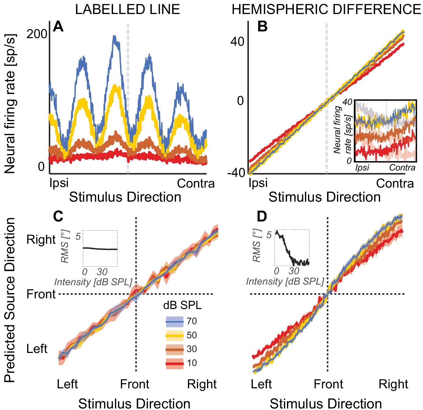
Modeling results.

(A) Firing rate of a simulated *nucleus laminaris* neuron with a preferred ITD of 375 µs, as a function of source ITD. The model predicts source laterality based on the locus of the peak of the firing rate function. (B) Hemispheric differences in firing rates, averaged across all 81 simulated *inferior colliculus* units. Rate models assume that source laterality is proportional to firing rate, causing ambiguities at the lowest sound intensities. Inset: Reconstructed responses of an *inferior colliculus* unit. The unit predominantly responds contralaterally to the direction of sound (high-contrast traces). The hemispheric difference model subtracts this activity from the average rate on the ipsilateral side (example shown with low-contrast traces). (C) Mean population response using labelled-line coding across a range of ITDs and sound intensities. Inset: The root-mean square (RMS) difference relative to estimated angle at 80 dB SPL does not change with sound intensity, predicting that sound laterality is intensity invariant. (D) Mean population response using hemispheric-difference coding. For lower sound intensities, predicted source direction is biased towards midline (compare red and orange versus blue or yellow). For higher sound intensities, predicted source direction is intensity invariant (blue on top of yellow line). Inset: RMS difference relative to estimated angle at 80 dB SPL decreases with increasing sound intensity, predicting that sound laterality is not intensity invariant. Ribbons show one standard error of the mean across 100 simulated responses. Sound intensity is denoted by color (see color key in the figure).

https://doi.org/10.7554/eLife.47027.003

A growing literature proposes an alternative to the labelled-line model to explain mammalian sensitivity to ITD (Lee and Groh, 2014). One reason for an alternative is that two excitatory inputs should suffice to implement the labelled-line model, but evidence from experiments on Mongolian gerbils shows that in addition to bilateral excitatory inputs, sharply tuned bilateral inhibitory inputs to the MSO play a crucial role in processing ITDs (Brand et al., 2002). Moreover, to date no labelled-line type neurons encoding auditory space have been discovered in a mammalian species. Indeed, using a population rate-code, several studies proposed that mammalian sound localization can be modeled based on differences in firing rates across the two populations of neurons that are tuned to opposing hemispheres (Figure 1B; van Bergeijk, 1962; McAlpine and Grothe, 2003; Devore et al., 2009). Rate-based models generally predict that neuronal responses carry most information at the steepest slopes of neural-discharge-rate versus ITD curves, where neural discharge changes most strongly (Stecker et al., 2005), consistent with the observation that the peak ITDs of rate-ITD curves often fall outside the physiologically plausible range (McAlpine and Grothe, 2003; Grothe et al., 2010; but see also Joris et al., 2006). In addition, some authors have suggested that how mammalian sound localization adapts to stimulus history further supports a rate-based neural population code, as assessed behaviorally or via magnetoencephalography (Phillips and Hall, 2005; Stange et al., 2013; Salminen et al., 2010).

It is unknown which of the two competing models, broadly characterized as labelled-line versus rate-code model, describes human sound localization better. Here, we observe that the two different models predict different dependencies of sound localization on sound intensity. By combining behavioral data on sound intensity dependence in normal-hearing listeners with numerical predictions of human sound lateralization from both models, we attempt to disentangle whether human auditory perception is based on a place-code, akin to the labelled-line model, or whether it is instead more closely described by a population rate-code.

An extensive physiology literature characterizes labelled-line versus population-rate type neurons and suggests that, at least from the perspective of evolution, birds and mammals use different neural mechanisms to calculate sound direction (review: Grothe, 2003). Thus, we searched the avian and mammalian physiology literature and identified two studies that characterized labelled-line versus population rate-code neurons at low sound levels and as a function of both sound level and ITD (Peña et al., 1996; Zwiers et al., 2004). Both Peña et al. (1996) and Zwiers et al. (2004) report neural firing rate in response to acoustic noise stimuli and are thus suitable for predicting each model’s sensitivity to the acoustic noises we tested in the current study. Here, we ran a meta-analysis, reconstructing simulated neurons with response characteristics from each of the two studies and using maximum likelihood estimation to predict source laterality from these previous findings.

Results

Model Predictions

To predict how lateralization depends on sound intensity from the responses of labelled-line neurons, we estimated neural firing rates from previous recordings in the nucleus laminaris in barn owl (Peña et al., 1996). To estimate lateralization’s dependence on level based on a population rate-code, we used previous recordings from the inferior colliculus of rhesus macaque monkey and calculated hemispheric differences in firing rate (Zwiers et al., 2004). The labelled-line neurons predicted that, as sound intensity decreases, perceived source laterality would converge towards similar means for low versus high sound intensities, with increased response variability at decreasing sound intensities (Figure 1C). In contrast, the hemispheric-difference model predicted that as sound intensity decreases to near threshold levels, perceived laterality would become increasingly biased toward the midline reference (Figure 1D, for example note the shallower slope and thus compressed laterality percepts for red versus blue curves). At higher overall sound intensities, both models predicted that lateralization would be intensity invariant (see insets in Figure 1C versus D). Therefore, analyzing how sound intensity affects perceived sound direction near sensation threshold offers an opportunity to disentangle whether our human auditory system relies on a place-based or rate-based population code for localizing sound based on ITD.

A listener’s ability to discriminate ITD can vary with sound intensity (Dietz et al., 2013). However, it is difficult to interpret previous findings linking sensitivity to ITD and a listener’s judgement of sound source direction as a function of sound intensity. Some reported decreased perceived source laterality near sensation threshold (Teas, 1962; Sabin et al., 2005), but others reported weak or no level effects on perceived lateralization (Von Békésy and Wever, 1960; Mickunas, 1963; Hartmann and Rakerd, 1993; Macpherson and Middlebrooks, 2000; Inoue, 2001; Vliegen and Van Opstal, 2004; Brungart and Simpson, 2008; Gai et al., 2013). Several factors complicate the interpretation of these previous findings in the context of the current hypothesis. For instance, assuming an approximately 30 dB dynamic range of rate-level function either at the MSO or downstream in the binaural pathway (e.g. medial superior olive: Goldberg and Brown, 1968; inferior colliculus: Zwiers et al., 2004), for stimuli at higher sensation levels (SL) where the rate-level functions saturate, both the labelled-line and the hemispheric difference model predict level invariance. This could explain how studies that tested for the role of sound level over a range of high intensities did not see an effect. Moreover, when presented in the free field, sounds also contain interaural level differences and spectral cues, in addition to ITD. For low-frequency sound, listeners rely dominantly on ITD when judging lateral source angle. However, for broadband sound, listeners integrate across all three types of spatial cue (Wightman and Kistler, 1992; Ihlefeld and Shinn-Cunningham, 2011). Unlike ITDs, interaural level differences and overall sound intensity both decrease with increasing source distance, raising the possibility that for stimuli with high-frequency content, listeners judged softer sounds to be more medial because they interpreted them to be farther away than louder sounds. Further, at low sound intensities, the sound-direction-related notches of the spectral cues at high-frequencies should have been less audible than at higher sound intensities, increasing stimulus ambiguity. A resulting increase in response variability may have obscured the effect of sound intensity on ITD coding. Finally, some historic studies used only two or three listeners, suggesting that they may have been statistically underpowered. Thus, the literature provides insufficient evidence on how ITD-based lateralization varies with sound level near sensation threshold.

Human perception

Here, we contrasted two competing hypotheses toward the goal of disentangling whether ITD-based human sound localization relies on a labelled-line versus a population rate-place neural code. The labelled-line code hypothesis predicted that the mean perceived direction based on ITD would be intensity invariant, even at intensities close to SL. Using a psychophysical paradigm, we studied lateralization based on ITD as a function of sound intensity in a group of ten normally hearing listeners (experiment 1). Stimuli consisted of low-frequency noise tokens that were bandlimited to cover most of the frequency range where humans can discriminate ITD (Brughera et al., 2013; here, corner frequencies from 300 to 1200 Hz, shown in Figure 2A). In each one-interval trial, listeners had to indicate perceived laterality across a range of ITDs from −375 to 375 μs. Lateralization was measured as function of SL. To examine how sound intensity affects perceived ITD coding of source direction, we modelled perceived laterality with a nonlinear mixed effect model (NLME) that included fixed effects of ITD and sound intensity as well as a random effect of listener.

Figure 2

Download asset Open asset

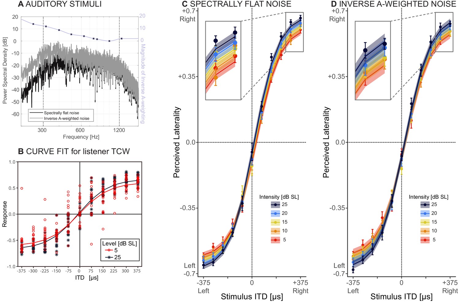
Behavioral results.

(A) Stimuli: spectrally flat noise, used in experiment 1 (dark grey) versus A-weighted noise, tested as a control for audibility in experiment 2 (light grey). The purple line shows the magnitude of the zero-phase inverse A-weighting filter. (B) Responses from one representative listener (TCW) across two sound intensities and the corresponding NLME fits for these data. (**C and D**) Perceived laterality as a function of ITD for C) spectrally flat noise (experiment 1) or D) A-weighted noise (experiment 2). Error bars, where large enough to be visible, show one standard error of the mean across listeners. Colors denote sound intensity. Insets illustrate magnified section of the plots. Circles show raw data, lines and ribbons show NLME fits and one standard of the mean.

https://doi.org/10.7554/eLife.47027.004

Figure 2B depicts lateralization performance with spectrally flat noise at two sound intensities for a representative listener (TCW). Figure 2C shows raw data (circles) and NMLE fits (lines) across all listeners. Error bars show one standard error of the mean across listeners, and shaded ribbons indicate one standard error of the mean fit across listeners. This model predicts 80.6% of the variance in the measured responses and is deemed an appropriate fit of the data. Table 1 lists all NLME parameters. Perceived laterality scores increased with increasing ITD, as expected. With decreasing sound intensity, percepts were increasingly biased towards midline (compare order of colored lines, magnified in the inset of Figure 2C). These trends were supported by the NLME model, which revealed significant effects of ITD (p<0.001; $α_{x 1}$ ) and sound intensity (p<0.001; $α_{y 1}$ ) on the maximal extent of laterality, confirming the predicted trend from the hemispheric difference model and rejecting our null hypothesis. Average pure tone audiometric thresholds affect perceived laterality, albeit mildly (p<0.001; $α_{y 2}$ = 0.01). Sound intensity did not significantly affect the slope of the psychometric functions (p=0.14; $α_{x 2}$ ).

Table 1

Results of Nonlinear Mixed Effects Model for flat-spectrum noise condition.

Note that Laterality:sound intensity refers to the NLME weight attributed to acoustic sound intensity of the auditory target. In contrast, Laterality:audibility captures the NLME weight attributed to pure tone audiometric thresholds based on the listeners’ perceptual abilities (see Materials and methods for details).

https://doi.org/10.7554/eLife.47027.005

Description		Value	Std.error	t-value	p-value
Intercept: ITD	$α_{x 0}$	0.06	0.04	1.58	0.11
Slope: ITD	$α_{x 1}$	2.45	0.05	46.15	<0.001	***
Slope: sound intensity	$α_{x 2}$	0.02	0.01	1.47	0.14
Laterality: sound intensity	$α_{y 1}$	0.05	0.01	7.59	<0.001	***
Laterality: audibility	$α_{y 2}$	0.01	0.002	4.86	<0.001	***

10986 degrees of freedom.

In a second experiment, we examined whether these results were robust to the spectral details of the stimuli. A caveat of testing spectrally flat noise at low sound intensities is that parts of the spectrum may be inaudible, and this may contribute to the slight but significant effect of audibility on laterality ( $α_{y 2}$ ). Therefore, the results of experiment 1 could potentially be confounded by the fact that the bandwidth of the audible portion of the noise tokens decreased with decreasing sound intensity. Alternatively, the effect of absolute pure tone detection thresholds that we observe in our normal-hearing listeners may reflect differences in neural function beyond audibility. As a control for perceived stimulus bandwidth, the same listeners were tested again, using inverse A-weighted noises (experiment 2). Inverse A-weighting boosts sound energy at each frequency in rough proportion to the human threshold. Resulting inverse A-weighted sensitivity thus achieves nearly constant sensation level across frequency. All of the original ten listeners from experiment 1 completed experiment 2. Methods were similar as in the first experiment, except that the stimuli consisted of inversely A-weighted noise (compare magnitude spectra in Figure 2A). The data and NLME model fits for the second experiment are shown in Figure 2D (color key identical to Figure 2C), and coefficients are listed in Table 2. This second model accounts for 80.4% of the variance in the data, closely fitting the measured responses. All NLME coefficients are significant (p<0.001 for $α_{x 1}$ ; $α_{x 2}$ ; $α_{y 1}$ and $α_{y 2}$ ). The intercept coefficient ( $α_{x 0}$ estimate = −0.60, SE = 0.03, p<0.001) revealed a slight leftward response bias, consistent with a slight narrowband interaural level difference in our stimuli due to precision limits of our test system. The fact that $α_{x 2}$ is significant shows that when all noise portions are approximately equally audible, as here, with inverse A-weighted noise, both perceived laterality and the slope linking the change in laterality to ITD decrease with decreasing sound intensity. This is consistent with the interpretation that by controlling for audibility across-frequency, the sensitivity of the task to sound level increases, revealing a medial bias effect not only for the most lateral but also for more medial source angles.

Table 2

Results of Nonlinear Mixed Effects Model for inverse A-weighted noise condition.

https://doi.org/10.7554/eLife.47027.006

NLME weight		Value	Std.error	t-value	p-value
Intercept: ITD	$α_{x 0}$	−0.60	0.03	−19.28	<0.001	***
Slope: ITD	$α_{x 1}$	2.57	0.06	46.26	<0.001	***
Slope: sound intensity	$α_{x 2}$	0.06	0.01	4.98	<0.001	***
Laterality: sound intensity	$α_{y 1}$	0.04	0.01	7.10	<0.001	***
Laterality: audibility	$α_{y 2}$	0.01	0.002	3.30	<0.001	***

10986 degrees of freedom.

Thus, the results confirm the effect of biasing perceived laterality toward midline with decreasing sound intensity. Therefore, for both spectrally flat noise and A-weighted noise, statistical analyses, which partialed out overall differences between listeners, are inconsistent with a labelled-line model of human sound localization.

Discussion

Population rate-coding to compute sensory dimension may not be unique to the auditory system. In analogy to sound localization based on the comparison of signals from the two ears (Figure 3A), visual depth is computed in the cerebral cortex based on signals from the two eyes (Figure 3B; Poggio, 1995; Parker and Cumming, 2001; Parker, 2016). Specifically, in both primary V1 and extrastriate V3a cortex of rhesus macaque monkeys, three types of neurons are thought to encode binocular disparity. ‘Tuned-excitatory’ neurons respond best to zero spatial disparity between the two eyes, whereas ‘near cells’ respond more vigorously when an object approaches, increasing crossed disparity between the eyes (Parker and Cumming, 2001). Finally, ‘far cells’ fire more vigorously as uncrossed disparity increases. In V1, the most frequently encountered type of binocular neurons are of the tuned-excitatory type. However, in V3a the large majority of neurons is stereo-specific (Poggio et al., 1988) and most neurons are either near or far cells. Functional magnetic resonance imaging experiments on human stereoscopic vision found that unlike V1 activity, the activity in cortical area V3a predicts behavioral performance on tasks involving stereoscopic depth (Backus et al., 2001). These observations lead us to propose that in order to compute perceptual space from sensory input, the central nervous system has evolved a canonical computation that is common to different sensory modalities. Specifically, we propose that near and far cells encode visual distance from the fixation plane in a way similar to how inferior colliculus neurons encode auditory azimuthal angle away from midline reference: firing rate increases monotonically with distance from perceptual reference anchor or fixation.

Figure 3

Download asset Open asset

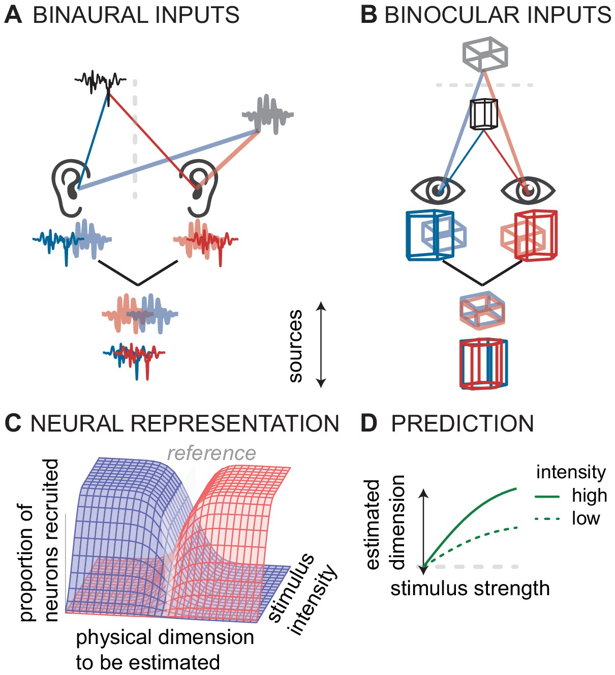
Conceptual model of canonical computation of location.

(A) Computing sound direction requires analysis of the binaural difference between the signals reaching the left and right ear. (B) Estimating visual depth hinges on analysis of the binocular disparity between the signals reaching left and right eye. (C) For both hearing and vision, the proportion of the neural population that is stimulated (in the *inferior colliculus* or V3) depends both on the physical dimension to be estimated (source laterality or source distance) and the intensity of the stimulus (sound intensity or visual contrast). For hearing and vision, ambiguity in this putative neural code predicts D) biased responses at low stimulus intensities (sound intensity or contrast).

https://doi.org/10.7554/eLife.47027.007

We observe that in both the auditory and the visual system, the same cells that are tuned to binaural ITD or binocular disparity also have intensity-response functions. A rate-code based on a population of these cells should cause ambiguities when stimulated below the saturation firing rate, either at low sound intensity or at low contrast (Figure 3C). Thus, based on the analogies between the stereo-depth computation and the azimuth-ITD computation, we hypothesized that low visual contrast might affect the computation of depth in a manner analogous to the effect of low sound levels in sound localization—there might be a bias to lower perceived depth at lower contrast (Figure 3D). Indeed, one study found such an effect, but only in some observers (Cisarik and Harwerth, 2008). A confounding factor in that earlier study is that perceived depth is a complicated neural computation, not only dependent on stereoscopic disparity but also on monocular cues including contrast (Parker, 2016). Several studies on depth perception indicate that low contrast is interpreted by the brain as a cue for distance; lower contrast targets are perceived farther away (e.g. Schor and Howarth, 1986; Rohaly and Wilson, 1999). However, experiments that controlled for low contrast bias demonstrated that low contrast causes perceived depth to shrink, both for near and far deviations from baseline (Chen et al., 2016). Thus, there is a link between population rate-coding and stimulus intensity in perceived visual depth as in perceived auditory azimuth, two perceptual spatial dimensions computed by the brain.

To illustrate how rate-based decoding of target location varies with sound intensity, we here chose a rate-coding model that compares firing rates across two populations of neurons, tuned to opposite hemifields. This read-out is a direct realization of the original canonical rate-based model for ITD decoding (van Bergeijk, 1962). Alternative rate-code readouts exist (for a recent summary of binaural models, see Dietz et al., 2018). Most of these rate-code models rely on subtractive comparisons between populations of neurons that are tuned to opposite hemifields, inherently sharing ambiguous readouts at low suprathreshold sound intensities. In contrast, divisive comparisons between ipsi- and contralaterally tuned neural populations are less likely to predict the observed behavioral bias due to stimulus intensity (Groh, 2001). Future work will need to delineate how specific implementations of rate-based readouts shape the intensity-induced bias of sound localization. Moreover, it has been suggested that depending on perceptual task, the mammalian brain could combine place- and rate-codes (Porter and Groh, 2006; Goodman et al., 2013). For instance, the mammalian auditory pathway may convert place- into rate-codes and vice versa (Groh et al., 2003; Porter and Groh, 2006). However, downstream from the inferior colliculus, rate-coding seems to be maintained, at least in the superior colliculus of rhesus macaque (Werner-Reiss and Groh, 2008; Lee and Groh, 2014). Moreover, our psychophysical and computational results suggest that for sound localization based on ITD at low sound levels, cortical maps do not play a role. However, there is good evidence for spatial map-like signals in higher order auditory cortical fields when interaural level differences are present, at medium to high sound levels (Higgins et al., 2010). How these interaural-level-difference-based cortical maps influence sound localization behavior is yet to be determined.

An additional factor restricting rate-based readouts is that auditory cortex units display nonlinear rate-intensity functions. For instance, excitatory-excitatory (EE) cells in auditory cortex that are tuned to sound locations near midline are also often tuned for sound intensity (Semple and Kitzes, 1993; Pollak et al., 2002; Zhang et al., 2004; Razak and Fuzessery, 2010; Higgins et al., 2010). This intensity tuning may complicate rate-based decoding at higher sound intensities. However, it is not apparent at the very low sound intensities needed to explain the perceptual bias observed here. There are additional fascinating findings in the neurophysiological literature regarding frequency and intensity tuning, and interesting correlations between non-monotonicity in the azimuthal and intensity dimensions (Woods et al., 2006), but a detailed discussion of these points is beyond the scope of the present behavioral-computational study.

In summary, unlike predictions from a rate-code neuronal readout, labelled-line coding predicts that sound localization is intensity invariant. Our experimental results show that for low frequency noise, where ITDs are the dominant localization cue, and at low sound intensities, sound lateralization based on ITD is not intensity invariant; it becomes increasingly medially biased with decreasing SL. The observed localization bias is overall small in magnitude, showing that the brain can robustly localize based on ITD across a large range of sound intensities. However, this bias is of theoretical importance as it confirms the prediction of a subtractive rate-based neuronal readout. Moreover, our auditory finding parallels a phenomenon of visual fixation bias when calculating visual distance from binocular disparity at low contrast. This casts doubt on the idea that the neural mechanism of ITD-based sound localization and binocular disparity-based visual distance estimation are based on place-based coding. Instead, our perceptual data on auditory localization together with previously published data on visual distance perception are parsimonious with the idea that a population rate-code underlies the brain’s computation of location.

Materials and methods

Experimental model and subject details

Request a detailed protocol

Twelve naïve normal-hearing listeners (ages 18–27, five females) were enrolled in this study and paid for their time. Their audiometric thresholds, as assessed via a calibrated GSI 39 Auto Tymp device (Grason-Stadler), were 25 dB hearing level or better at octave frequencies from 250 to 8000 Hz, and did not differ by more than 10 dB across ears at each octave frequency. This study was approved by and all testing was administered according to the guidelines of the Institutional Review Board of the New Jersey Institute of Technology, protocol F217-14. All listeners gave written informed consent both to participate in the study and to publish the results with confidential listener identity.

Method details

Request a detailed protocol

Listeners were seated in a double-walled sound-attenuating booth (Industrial Acoustics Company) with a noise floor of 20.0 dB SPL (wideband LAFeq). Stimuli were digitally generated in Matlab R2016b (The MathWorks, Inc), D/A converted through an external sound card (Emotiva Stealth DC-1) at a sampling frequency of 192 kHz, with a resolution of 24 bits per sample, and presented to the listener through ER-2 insert earphones (Etymotic Research Inc). The equipment was calibrated using an acoustic mannequin (KEMAR model, G.R.A.S. Sound and Vibration) with a precision of less than ±5 μs ITD and less than ±1 dB interaural level difference. Foam eartips were inserted following guidelines provided by Etymotic Research to encourage equal representation of sounds to both ears and minimize interaural leakage. Each session lasted approximately 60 min. Listeners kept the insert earphones placed inside their ears throughout testing. Insert earphones were replaced by the experimenter after each break. Throughout this study, to generate stimuli, tokens of uniformly distributed white noise were generated and bandpassed using a zero-phase Butterworth filter with 36 dB/octave frequency roll-off, and 3 dB down points at 300 and 1200 Hz. Each noise token was 1 s in duration, including 10 ms long squared cosine ramps at the onset and offset.

Sensation level measurements

Request a detailed protocol

At the beginning of each session, and, as a re-test control, mid-way through each session, each individual listener’s SL was measured for the type of sound that was later on used for training and testing, via one run of adaptive tracking. On each one-interval trial of each track, a new noise token was generated and presented diotically. Trials were spaced randomly in time (uniform distribution, inter-token intervals from 3 to 5.5 s). Listeners pressed a button when they heard a sound. No response feedback was given.

On each trial, a response was scored a ‘hit’ if a listener responded with a button push before the onset of the subsequent trial, and a ‘miss’ if the listener did not respond during the interval. If a listener’s response changed from hit to miss or from miss to hit across sequential trials, this was interpreted as a response reversal. Using one-up-one-down adaptive tracking, the noise intensity was increased or decreased after each reversal, with a step size of 5 dB (decreasing) or 2.5 dB (increasing). Each listener completed ten adaptive-track reversals, with SL threshold equaling the median of the final six reversals. Each SL was used as reference intensity for the subsequent 30 min of testing. If detection thresholds changed between initial test and re-test control by more than 5 dB, this indicated that an insert earphone moved, and the experimenter replaced the earphones. Thresholds generally did not change by more than 5 dB.

Training

Request a detailed protocol

To train listeners on consistently reporting their perception of ITD, using adaptive tracking, listeners matched the perceived laterality of a variable-ITD pointer to that of a fixed-ITD target. Target token intensity was set relative to the listener’s own diotic sensation threshold, at 10 or 25 dB SL, and presented with 0 dB interaural level difference. The pointer intensity was fixed at 25 dB SL. Target ITDs spanned the range from −375 to 375 μs, in 75 μs steps. Target ITDs and SLs were randomly interleaved across runs, but held fixed throughout each adaptive run. In each two-interval trial of a run, the pointer token was presented in the first, and the target token in the second interval. The start ITD of the pointer token at the beginning of each run equaled 0 μs. Using a hand-held controller (Xbox 360 wireless controller for Windows, Microsoft Corp.), listeners adjusted the ITD of the pointer token. Specifically, listeners pushed the directional keys (D-pad) either to the left or right in order to move and match the pointer direction with that of the target sound. When a listener indicated a left- or right-ward response, the pointer ITD was decreased or increased. Initial ITD step size equaled 100 μs, then 50 ±5 μs (uniformly distributed) after the first reversal. By the end of the second reversal, ITD step size was reduced to 25 ±5 μs (uniformly distributed) and remained the same for all of the following reversals. Listeners were instructed to ‘home in’ on the target by moving the pointer initially to a position more lateral than the target, then more medial than the target with the goal of centering on the target. No response feedback was provided. A run was completed after a listener had completed a total of five adaptive-tracking reversals. For each target ITD, the matched pointer ITD was estimated by averaging the pointer ITDs of the final two reversals. Each listener performed three sessions of training: In the first session only a subset of target ITDs were presented (−375,–150, 0, 150 and 375 μs), whereas the two following sessions included all of the eleven ITDs. Per training session, each ITD was presented once at 10 and 25 dB SL, for a total of 54 adaptive tracking runs across all training sessions. To familiarize listeners with the experimental task (described below), at the end of second and third sessions of training listeners performed an additional 5 blocks of the experimental testing task, without response feedback. These task training data were not used for statistical analysis.

To assess whether listeners could reliably report their lateralization percepts, training performance was evaluated for each listener by calculating the Pearson correlation coefficient between target ITD and matched pointer ITD in the final training session. Criterion correlation equaled 0.9 (N = 11 ITDs, significance level = 0.01, power = 0.95). Ten listeners reached criterion, suggesting that they were able to consistently report where they perceived the sounds based on ITD. Two of the originally recruited twelve listeners failed to reach training criterion ( $R^{2}$ = <0.84, 0.87>) and were excluded from testing.

Testing

Request a detailed protocol

Using the method of fixed stimuli, we tested lateralization in two experiments. Except for the stimuli, which consisted of spectrally flat noise tokens in experiment 1 and A-weighted noise tokens in experiment 2, the methods were similar across the two experiments. Noise tokens were generated from a statistically similar noise distribution as those presented during both SL measurements and training (see Overall Design). A touchscreen monitor (Dell P2314T) displayed the response interface at about 40 cm distance from the listener. Using a precise touch stylus (MEKO Active Fine Point Stylus 1.5 mm Tip), listeners indicated perceived laterality of noise in a one-interval task. Noise tokens were presented at 5, 10, 15, 20, and 25 dB SL. ITDs varied randomly from trial to trial, in 75 μs steps spanning the range from −375 μs to 375 μs. On each trial, a new token of noise was generated. Each listener performed 20 blocks of 55 trials each (11 ITDs at each of the five sound intensities), with SL measured both before the first and the eleventh block. ITDs and sound intensity were randomly interleaved from trial to trial such that each combination of ITD and sound intensity was presented once before all of them were repeated in a different random order.

Models

Request a detailed protocol

We estimate the combined effects of ITD and sound intensity on predicted source laterality both in avian labelled-line type units and in binaurally sensitive units of a mammalian auditory system. The sound intensities where we expect to see an effect of overall sound level fall below 30 dB SPL, because only in this range would most auditory neurons fire below saturation, allowing us to disambiguate labelled-line versus hemispheric rate-difference coding. However, scant data exist for either type of unit at sound pressure levels below 30 dB SPL. We identified two prior studies that have measured neural discharge rate as a function of ITD at these very low sound intensities. Both studies used noise as acoustic stimuli, and the neural response statistics they report are thus suitable for estimating what type of information would be available to either type of coding mechanism with the type of noise stimuli that human listeners lateralized in the behavioral experiments here.

One study in barn owl shows that the output functions of nucleus laminaris neurons can be modeled through interaural cross-correlation functions, even at very low sound intensities (Peña et al., 1996). That study reports Pearson correlation coefficients between the neural response function of nucleus laminaris units at 50 dB SPL versus all other tested sound levels. To reconstruct the spatial information realistically available from the output of labelled-line neurons, across both a range of −375 to 375 μs ITD in 20 μs steps, we first constructed biologically plausible interaural cross-correlation functions at 50 dB SPL and then added internal noise to the resulting curves to mimic the Pearson correlation coefficients reported by Peña et al. (1996). Our model predictions pertain to sound intensities spanning the range from 10 to 70 dB SPL, similar to previous work (Peña et al., 1996). Due to overall scarcity of available data at low dB SPL, here we use firing rate characteristics for unit # 0123795–530.02 (Peña et al., 1996) with a nominal best frequency of 1 kHz. To generate the acoustic inputs to the labelled-line model, we initially generated a Gaussian noise token, duplicated it and introduced a variable ITD, spanning a range from −375 to 375 μs, with 20 μs step size and 0 dB interaural level difference. To simulate ITD information available after cochlear processing, we then processed both noises with a 1/3-octave wide bandpass filter with 24 dB/octave frequency roll-off, followed by half-wave rectification and low-pass filtering at 1500 Hz. We then simulated internal noise by adding uniformly distributed dichotic noise tokens with mean spontaneous firing rates of 5% of the root mean square value of the signal, resulting in left (L) and right (R) inputs to the binaural cross-correlation neurons, called $x_{L} (t)$ and $x_{R} (t)$ . To establish 50 dB SPL reference functions, at each simulated ITD, we then calculated the binaural cross-correlation function $c c (τ)$ of $x_{L} (t)$ and $x_{R} (t)$ , as follows: $c c (τ) = 300 + (450 - 300) \frac{\int_{- \infty}^{+ \infty} x_{L} (t) x_{R} (t + τ) d t)}{m a x | \int_{- \infty}^{+ \infty} x_{L} (t) x_{R} (t + τ) d t |}$ , with $τ$ signifying the best ITD of each neuron, and extrema scaled such that $c c (τ)$ spans a range from 300 to 450 spikes/sec, approximating nucleus laminaris firing rates at 50 dB SPL (Peña et al., 1996). To simulate non-sound driven neural discharge, we then added uniformly distributed random noise ${\hat{c c}}_{r e f} (τ) = c c (τ) + U (0, μ)$ , with a mean discharge of $μ$ = 5 spikes/sec, (Peña et al., 1996). The resulting signal is our reference cross-correlation function at 50 dB SPL, called $c c_{r e f} (τ)$ , shown in Figure 1A as yellow bold line for a representative simulated neuron.

For each sound level and ITD, we then statistically reconstructed a family of interaural cross-correlation functions that match the originally reported functions (Peña et al., 1996). Specifically, we added scaled dichotic uniformly distributed noise tokens $n_{L} (t) \leftarrow U (0, μ)$ and $n_{R} (t) \leftarrow U (0, μ)$ to the $x_{L} (t)$ and $x_{R} (t)$ , such that the monaural inputs to the binaural cross-correlation functions equal ${\hat{x}}_{L, R} (t) = α x_{L, R} (t) + \sqrt{1 - α^{2}} n_{L, R} (t)$ . The resulting cross-correlation function for each sound level and ITD is then $\hat{c c} (τ) = (x_{L} ⋆ x_{R}) (τ)$ , shown for a representative neuron in Figure 1A as blue, brown and red lines corresponding to 70, 30 and 10 dB SPL. We then searched through the space of scaling coefficients $α$ until the Pearson correlation coefficient between $c c_{r e f} (τ)$ and $\hat{c c} (τ)$ matched the coefficients originally reported by Peña et al. (1996) with a precision error of less than 10%.

To estimate predicted sound laterality as a function of sound intensity for these simulated labelled-line neurons, at each intensity, we then identified the $τ$ where $\hat{c c} (τ) = m a x (\hat{c c} (τ))$ . For each sound level and ITD, we calculated predicted sound laterality in 100 repetitions of these simulations. Figure 1C shows mean estimated laterality across these 100 simulations, with ribbons showing one standard error of the mean across simulations.

To estimate source laterality based on rate-coding, we assayed the mammalian auditory system, where one previous study reports firing statistics for 81 inferior colliculus units in rhesus macaque as a function of ITD and over a wide range of sound intensities, including very low sound intensities (Zwiers et al., 2004). From the previously published linear regression parameters, we initially reconstruct linear regression functions linking ITD, sound intensity and firing rate (Zwiers et al., 2004). However, while linear regression fits afford statisticial convenience, they cannot fully capture the sigmoidally shaped firing rate functions in mammalian inferior colliculus units. Therefore, we multiplied the original linear reconstructions with sigmoid functions. Specifically, consistent with prior literature, each simulated sigmoidal output function saturates over a 30 dB dynamic range, has linear growth over the physiologically plausible range of contralateral ITDs, has a threshold between uniformly distributed between 0 and 10 dB SPL, and a spontaneous non-sound-evoked discharge of between 2 and 10 spikes/second (e.g. Ramachandran et al., 1999).

The inset of Figure 1B shows a representative simulated inferior colliculus unit (color denotes sound intensity, dark shading shows contralateral responses), whereas Figure 1B shows the differences in firing rates for contra minus ipsi-lateral simulated firing rates, averaged across all 81 simulated inferior colliculus units. From these resulting differences in contra versus ipsi firing rates we calculated, collapsed across sound intensities from 0 to 80 dB SPL, the probability density of the firing rate for each inferior colliculus unit as a function of source ITD. Assuming an ideal observer, we then classified the sound azimuth as a function of sound intensity via maximum likelihood estimation. To calculate the mean and variance of predicted ITD as a function of sound intensity, we then ran a bootstrapping analysis, sampling with replacement 100 times. Figure 1D shows the across-simulation average predicted source laterality, with ribbons showing one standard error of the mean across simulations.

Quantification and statistical analysis

Request a detailed protocol

Growth curve analysis was used to analyze perceived laterality scores as a function of ITD and sound intensity. For each of the two noise conditions, the perceived laterality scores were fitted with an NLME model. The model included fixed effects $α$ and random effects $β$ . Equation 1 describes a sigmoidal function linking ITD to perceived laterality, with a score from left (−1) to right (1). The effect of sound intensity on the maximal extent of lateralization is $α_{y 1}$ . To factor out across-listener differences in absolute hearing thresholds, for each listener, we calculated the pure tone average (PTA) detection threshold in quiet, averaged across ears, and across 500 and 1000 Hz. Weight $α_{y 2}$ models the contribution of PTA. The slope terms are $α_{x 1}$ for perceived laterality changes attributed to ITD, and $α_{x 2}$ for laterality-ITD slopes attributed to sound intensity. Our stimuli were initially calibrated to have a broadband interaural level difference of 0 dB. However, because the transfer function of our sound card was not perfectly flat across frequency, fluctuations of ±1 dB interaural level difference occurred across frequency, on the same order of magnitude as the minimal threshold for human interaural level difference discrimination (Francart and Wouters, 2007). Thus, parameter $α_{x 0}$ factors out central response bias from the lateralization scores. Random effects of individual differences across listeners were used to model both the maximal extent of lateralization, $β_{y 0, l i s t e n e r}$ , and the perceived midline, $β_{x 0, l i s t e n e r}$ , centering the sigmoid (Equation 1):

r e s p o n s e \sim \frac{α_{y 2} \times P T A + α_{y 1} \times i n t e n s i t y + β_{y 0, l i s t e n e r}}{1 + e^{- [α_{x 2} \times i n t e n s i t y + α_{x 1} \times (I T D - α_{x 0} - β_{x 0, l i s t e n e r})]}} - 0.5

To better conform with the assumptions of the NLME model, prior to fitting, ITD and sound intensity parameters were scaled by subtracting the mean stimulus value, and dividing by the standard deviation of stimulus parameters, resulting in distributions of stimulus parameters with zero-mean and a variance of one. Laterality scores were then fitted using these normalized parameters, with the nlme package, programmed in RStudio 1.1 for Windows (RStudio Inc, Boston, MA, USA).

Data and software availability

Request a detailed protocol

All data and analysis code are available at Dryad (http://doi.org/10.5061/dryad.t8c381f) .

Data availability

The computational models, coded in Matlab, and all raw data generated or analysed during this study together with the statistical model, coded in R, have been provided via Dryad (http://doi.org/10.5061/dryad.t8c381f).

The following data sets were generated

(2019) Dryad Digital Repository
Data from: Human sound localization depends on sound intensity: implications for sensory coding.

https://doi.org/10.5061/dryad.t8c381f

References

(2001) Human cortical activity correlates with stereoscopic depth perception
Journal of Neurophysiology 86:2054–2068.

https://doi.org/10.1152/jn.2001.86.4.2054
- PubMed
- Google Scholar
1. Batra R
2. Yin TC
(2004) Cross correlation by neurons of the medial superior olive: a reexamination
Journal of the Association for Research in Otolaryngology 5:238–252.

https://doi.org/10.1007/s10162-004-4027-4
- PubMed
- Google Scholar
1. Brand A
2. Behrend O
3. Marquardt T
4. McAlpine D
5. Grothe B
(2002) Precise inhibition is essential for microsecond interaural time difference coding
Nature 417:543–547.

https://doi.org/10.1038/417543a
- PubMed
- Google Scholar
(2001) Binaural processing model based on contralateral inhibition. I. model structure
The Journal of the Acoustical Society of America 110:1074–1088.

https://doi.org/10.1121/1.1383297
- PubMed
- Google Scholar
(2013) Human interaural time difference thresholds for sine tones: the high-frequency limit
The Journal of the Acoustical Society of America 133:2839–2855.

https://doi.org/10.1121/1.4795778
- PubMed
- Google Scholar
Conference
1. Brungart DS
2. Simpson BD
(2008)
Effects of temporal fine structure on the localization of broadband sounds: potential implications for the design of spatial audio displays

Proceedings of the 14 International Conference on Auditory Display.
- Google Scholar
1. Carr CE
2. Konishi M
(1988) Axonal delay lines for time measurement in the owl's brainstem
PNAS 85:8311–8315.

https://doi.org/10.1073/pnas.85.21.8311
- Google Scholar
1. Chen PY
2. Chen CC
3. Tyler CW
(2016) The perceived depth from disparity as function of luminance contrast
Journal of Vision 16:20.

https://doi.org/10.1167/16.11.20
- PubMed
- Google Scholar
1. Cisarik PM
2. Harwerth RS
(2008) The effects of interocular correlation and contrast on stereoscopic depth magnitude estimation
Optometry and Vision Science 85:164–173.

https://doi.org/10.1097/OPX.0b013e3181643e65
- PubMed
- Google Scholar
1. Day ML
2. Semple MN
(2011) Frequency-dependent interaural delays in the medial superior olive: implications for interaural cochlear delays
Journal of Neurophysiology 106:1985–1999.

https://doi.org/10.1152/jn.00131.2011
- Google Scholar
(2009) Accurate sound localization in reverberant environments is mediated by robust encoding of spatial cues in the auditory midbrain
Neuron 62:123–134.

https://doi.org/10.1016/j.neuron.2009.02.018
- PubMed
- Google Scholar
(2013) The effect of overall level on sensitivity to interaural differences of time and level at high frequencies
The Journal of the Acoustical Society of America 134:494–502.

https://doi.org/10.1121/1.4807827
- PubMed
- Google Scholar
1. Dietz M
2. Lestang JH
3. Majdak P
4. Stern RM
5. Marquardt T
6. Ewert SD
7. Hartmann WM
8. Goodman DFM
(2018) A framework for testing and comparing binaural models
Hearing Research 360:92–106.

https://doi.org/10.1016/j.heares.2017.11.010
- PubMed
- Google Scholar
1. Domnitz RH
2. Colburn HS
(1977) Lateral position and interaural discrimination
The Journal of the Acoustical Society of America 61:1586–1598.

https://doi.org/10.1121/1.381472
- PubMed
- Google Scholar
1. Durlach NI
(1963) Equalization and cancellation theory of binaural masking‐level differences
The Journal of the Acoustical Society of America 35:1206–1218.

https://doi.org/10.1121/1.1918675
- Google Scholar
1. Francart T
2. Wouters J
(2007) Perception of across-frequency interaural level differences
The Journal of the Acoustical Society of America 122:2826–2831.

https://doi.org/10.1121/1.2783130
- PubMed
- Google Scholar
1. Gai Y
2. Ruhland JL
3. Yin TCT
4. Tollin DJ
(2013) Behavioral and modeling studies of sound localization in cats: effects of stimulus level and duration
Journal of Neurophysiology 110:607–620.

https://doi.org/10.1152/jn.01019.2012
- Google Scholar
1. Goldberg JM
2. Brown PB
(1968) Functional organization of the dog superior olivary complex: an anatomical and electrophysiological study
Journal of Neurophysiology 31:639–656.

https://doi.org/10.1152/jn.1968.31.4.639
- PubMed
- Google Scholar
(2013) Decoding neural responses to temporal cues for sound localization
eLife 2:e01312.

https://doi.org/10.7554/eLife.01312
- PubMed
- Google Scholar
1. Groh JM
(2001) Converting neural signals from place codes to rate codes
Biological Cybernetics 85:159–165.

https://doi.org/10.1007/s004220100249
- PubMed
- Google Scholar
(2003) A monotonic code for sound azimuth in primate inferior colliculus
Journal of Cognitive Neuroscience 15:1217–1231.

https://doi.org/10.1162/089892903322598166
- PubMed
- Google Scholar
1. Grothe B
(2003) New roles for synaptic inhibition in sound localization
Nature Reviews Neuroscience 4:540–550.

https://doi.org/10.1038/nrn1136
- PubMed
- Google Scholar
(2010) Mechanisms of sound localization in mammals
Physiological Reviews 90:983–1012.

https://doi.org/10.1152/physrev.00026.2009
- PubMed
- Google Scholar
1. Hafter ER
(1971) Quantitative evaluation of a lateralization model of masking‐level differences
The Journal of the Acoustical Society of America 50:1116–1122.

https://doi.org/10.1121/1.1912743
- Google Scholar
(2005)
Binaural coherence in rooms

Acta Acustica United with Acustica 91:451–462.
- Google Scholar
1. Hartmann WM
2. Rakerd B
(1993) Auditory spectral discrimination and the localization of clicks in the sagittal plane
The Journal of the Acoustical Society of America 94:2083–2092.

https://doi.org/10.1121/1.407481
- PubMed
- Google Scholar
(2010) Specialization of binaural responses in ventral auditory cortices
Journal of Neuroscience 30:14522–14532.

https://doi.org/10.1523/JNEUROSCI.2561-10.2010
- PubMed
- Google Scholar
1. Ihlefeld A
2. Shinn-Cunningham BG
(2011) Effect of source spectrum on sound localization in an everyday reverberant room
The Journal of the Acoustical Society of America 130:324–333.

https://doi.org/10.1121/1.3596476
- PubMed
- Google Scholar
1. Inoue J
(2001) Effects of stimulus intensity on sound localization in the horizontal and upper-hemispheric median plane
Journal of UOEH 23:127–138.

https://doi.org/10.7888/juoeh.23.127
- PubMed
- Google Scholar
1. Jeffress LA
(1948) A place theory of sound localization
Journal of Comparative and Physiological Psychology 41:35–39.

https://doi.org/10.1037/h0061495
- PubMed
- Google Scholar
(2006) Binaural and cochlear disparities
PNAS 103:12917–12922.

https://doi.org/10.1073/pnas.0601396103
- PubMed
- Google Scholar
1. Lee J
2. Groh JM
(2014) Different stimuli, different spatial codes: a visual map and an auditory rate code for oculomotor space in the primate superior colliculus
PLOS ONE 9:e85017.

https://doi.org/10.1371/journal.pone.0085017
- PubMed
- Google Scholar
1. Macpherson EA
2. Middlebrooks JC
(2000) Localization of brief sounds: effects of level and background noise
The Journal of the Acoustical Society of America 108:1834–1849.

https://doi.org/10.1121/1.1310196
- PubMed
- Google Scholar
1. McAlpine D
2. Grothe B
(2003) Sound localization and delay lines--do mammals fit the model?
Trends in Neurosciences 26:347–350.

https://doi.org/10.1016/S0166-2236(03)00140-1
- PubMed
- Google Scholar
1. Mickunas J
(1963) Interaural time delay and apparent direction of clicks
The Journal of the Acoustical Society of America 35:788.

https://doi.org/10.1121/1.2142443
- Google Scholar
(1992) A circuit for coding interaural time differences in the chick brainstem
The Journal of Neuroscience 12:1698–1708.

https://doi.org/10.1523/JNEUROSCI.12-05-01698.1992
- PubMed
- Google Scholar
1. Parker AJ
(2016) Vision in our three-dimensional world
Philosophical Transactions of the Royal Society B: Biological Sciences 371:20150251.

https://doi.org/10.1098/rstb.2015.0251
- Google Scholar
1. Parker A
2. Cumming B
(2001)
Progress in Brain Research

205–216, Cortical mechanisms of binocular stereoscopic vision, Progress in Brain Research, 134, Elsevier, 10.1016/S0079-6123(01)34015-3.
- Google Scholar
1. Pecka M
2. Siveke I
3. Grothe B
4. Lesica NA
(2010) Enhancement of ITD coding within the initial stages of the auditory pathway
Journal of Neurophysiology 103:38–46.

https://doi.org/10.1152/jn.00628.2009
- PubMed
- Google Scholar
1. Peña JL
2. Viete S
3. Albeck Y
4. Konishi M
(1996) Tolerance to sound intensity of binaural coincidence detection in the nucleus laminaris of the owl
The Journal of Neuroscience 16:7046–7054.

https://doi.org/10.1523/JNEUROSCI.16-21-07046.1996
- PubMed
- Google Scholar
1. Phillips DP
2. Hall SE
(2005) Psychophysical evidence for adaptation of central auditory processors for interaural differences in time and level
Hearing Research 202:188–199.

https://doi.org/10.1016/j.heares.2004.11.001
- PubMed
- Google Scholar
(1988) Stereoscopic mechanisms in monkey visual cortex: binocular correlation and disparity selectivity
The Journal of Neuroscience 8:4531–4550.

https://doi.org/10.1523/JNEUROSCI.08-12-04531.1988
- PubMed
- Google Scholar
1. Poggio GE
(1995) Mechanisms of Stereopsis in monkey visual cortex
Cerebral Cortex 5:193–204.

https://doi.org/10.1093/cercor/5.3.193
- PubMed
- Google Scholar
1. Pollak GD
2. Burger RM
3. Park TJ
4. Klug A
5. Bauer EE
(2002) Roles of inhibition for transforming binaural properties in the brainstem auditory system
Hearing Research 168:60–78.

https://doi.org/10.1016/S0378-5955(02)00362-3
- PubMed
- Google Scholar
1. Porter KK
2. Groh JM
(2006) The "other" transformation required for visual-auditory integration: representational format
Progress in Brain Research 155:313–323.

https://doi.org/10.1016/S0079-6123(06)55018-6
- PubMed
- Google Scholar
(1999) Single-unit responses in the inferior colliculus of decerebrate cats. I. classification based on frequency response maps
Journal of Neurophysiology 82:152–163.

https://doi.org/10.1152/jn.1999.82.1.152
- PubMed
- Google Scholar
1. Razak KA
2. Fuzessery ZM
(2010) GABA shapes a systematic map of binaural sensitivity in the auditory cortex
Journal of Neurophysiology 104:517–528.

https://doi.org/10.1152/jn.00294.2010
- Google Scholar
1. Rohaly AM
2. Wilson HR
(1999) The effects of contrast on perceived depth and depth discrimination
Vision Research 39:9–18.

https://doi.org/10.1016/S0042-6989(98)00034-0
- PubMed
- Google Scholar
(2005) Human sound localization at near-threshold levels
Hearing Research 199:124–134.

https://doi.org/10.1016/j.heares.2004.08.001
- PubMed
- Google Scholar
(2010) The neural code for interaural time difference in human auditory cortex
The Journal of the Acoustical Society of America 127:EL60–EL65.

https://doi.org/10.1121/1.3290744
- Google Scholar
1. Schor CM
2. Howarth PA
(1986) Suprathreshold stereo-depth matches as a function of contrast and spatial frequency
Perception 15:249–258.

https://doi.org/10.1068/p150249
- PubMed
- Google Scholar
1. Semple MN
2. Kitzes LM
(1993) Focal selectivity for binaural sound pressure level in cat primary auditory cortex: two-way intensity network tuning
Journal of Neurophysiology 69:462–473.

https://doi.org/10.1152/jn.1993.69.2.462
- PubMed
- Google Scholar
1. Spitzer MW
2. Semple MN
(1995) Neurons sensitive to interaural phase disparity in gerbil superior olive: diverse monaural and temporal response properties
Journal of Neurophysiology 73:1668–1690.

https://doi.org/10.1152/jn.1995.73.4.1668
- PubMed
- Google Scholar
1. Stange A
2. Myoga MH
3. Lingner A
4. Ford MC
5. Alexandrova O
6. Felmy F
7. Pecka M
8. Siveke I
9. Grothe B
(2013) Adaptation in sound localization: from GABA(B) receptor-mediated synaptic modulation to perception
Nature Neuroscience 16:1840–1847.

https://doi.org/10.1038/nn.3548
- PubMed
- Google Scholar
(2005) Location coding by opponent neural populations in the auditory cortex
PLOS Biology 3:e78.

https://doi.org/10.1371/journal.pbio.0030078
- PubMed
- Google Scholar
1. Stern RM
2. Trahiotis C
(1995) Models of binaural interaction
Handbook of Perception and Cognition 6:347–386.

https://doi.org/10.1016/B978-012505626-7/50012-1
- Google Scholar
1. Teas DC
(1962) Lateralization of acoustic transients
The Journal of the Acoustical Society of America 34:1460–1465.

https://doi.org/10.1121/1.1918368
- Google Scholar
1. van Bergeijk WA
(1962) Variation on a theme of békésy: a model of binaural interaction
The Journal of the Acoustical Society of America 34:1431–1437.

https://doi.org/10.1121/1.1918364
- Google Scholar
1. Vliegen J
2. Van Opstal AJ
(2004) The influence of duration and level on human sound localization
The Journal of the Acoustical Society of America 115:1705–1713.

https://doi.org/10.1121/1.1687423
- PubMed
- Google Scholar
Book
1. Von Békésy G
2. Wever E
(1960)
Experiments in Hearing

New York: McGraw-Hill.
- Google Scholar
1. Werner-Reiss U
2. Groh JM
(2008) A rate code for sound azimuth in monkey auditory cortex: implications for human neuroimaging studies
Journal of Neuroscience 28:3747–3758.

https://doi.org/10.1523/JNEUROSCI.5044-07.2008
- PubMed
- Google Scholar
1. Wightman FL
2. Kistler DJ
(1992) The dominant role of low-frequency interaural time differences in sound localization
The Journal of the Acoustical Society of America 91:1648–1661.

https://doi.org/10.1121/1.402445
- PubMed
- Google Scholar
1. Woods TM
2. Lopez SE
3. Long JH
4. Rahman JE
5. Recanzone GH
(2006) Effects of stimulus azimuth and intensity on the single-neuron activity in the auditory cortex of the alert macaque monkey
Journal of Neurophysiology 96:3323–3337.

https://doi.org/10.1152/jn.00392.2006
- PubMed
- Google Scholar
1. Yin TC
2. Chan JC
(1990) Interaural time sensitivity in medial superior olive of cat
Journal of Neurophysiology 64:465–488.

https://doi.org/10.1152/jn.1990.64.2.465
- PubMed
- Google Scholar
(2004) Binaural interaction revisited in the cat primary auditory cortex
Journal of Neurophysiology 91:101–117.

https://doi.org/10.1152/jn.00166.2003
- Google Scholar
(2004) Involvement of monkey inferior colliculus in spatial hearing
Journal of Neuroscience 24:4145–4156.

https://doi.org/10.1523/JNEUROSCI.0199-04.2004
- PubMed
- Google Scholar

Article and author information

Author details

Antje Ihlefeld

New Jersey Institute of Technology, Newark, United States

Contribution
Conceptualization, Software, Formal analysis, Supervision, Funding acquisition, Methodology, Writing—original draft, Project administration, Writing—review and editing

For correspondence
antje.ihlefeld@njit.edu

Competing interests
No competing interests declared

"This ORCID iD identifies the author of this article:" 0000-0001-7185-5848
Nima Alamatsaz
1. New Jersey Institute of Technology, Newark, United States
2. Rutgers University, Newark, United States
Contribution
Software, Formal analysis, Investigation, Writing—review and editing

Competing interests
No competing interests declared

"This ORCID iD identifies the author of this article:" 0000-0003-3374-3663
Robert M Shapley

New York University, New York, United States

Contribution
Conceptualization, Methodology, Writing—review and editing

Competing interests
No competing interests declared

Funding

New Jersey Health Foundation (PC 24-18)

Antje Ihlefeld

The funders had no role in study design, data collection and interpretation, or the decision to submit the work for publication.

Ethics

Human subjects: This study was approved by and all testing was administered according to the guidelines of the Institutional Review Board of the New Jersey Institute of Technology, protocol F217-14. All listeners gave written informed consent both to participate in the study and to publish the results with confidential listener identity.

Copyright

This article is distributed under the terms of the Creative Commons Attribution License, which permits unrestricted use and redistribution provided that the original author and source are credited.