Science Forum: Ten common statistical mistakes to watch out for when writing or reviewing a manuscript
- University College London, United Kingdom
- KU Leuven, Belgium
Abstract
Inspired by broader efforts to make the conclusions of scientific research more robust, we have compiled a list of some of the most common statistical mistakes that appear in the scientific literature. The mistakes have their origins in ineffective experimental designs, inappropriate analyses and/or flawed reasoning. We provide advice on how authors, reviewers and readers can identify and resolve these mistakes and, we hope, avoid them in the future.
Main text
Much has been written about the need to improve the reproducibility of research (Bishop, 2019; Munafò et al., 2017; Open Science Collaboration, 2015; Weissgerber et al., 2018), and there have been many calls for improved training in statistical analysis techniques (Schroter et al., 2008). In this article we discuss ten statistical mistakes that are commonly found in the scientific literature. Although many researchers have highlighted the importance of transparency and research ethics (Baker, 2016; Nosek et al., 2015), here we discuss statistical oversights which are out there in plain sight in papers that advance claims that do not follow from the data – papers that are often taken at face value despite being wrong (Harper and Palayew, 2019; Nissen et al., 2016; De Camargo, 2012). In our view, the most appropriate checkpoint to prevent erroneous results from being published is the peer-review process at journals, or the online discussions that can follow the publication of preprints. The primary purpose of this commentary is to provide reviewers with a tool to help identify and manage these common issues.
All of these mistakes are well known and there have been many articles written about them, but they continue to appear in journals. Previous commentaries on this topic have tended to focus on one mistake, or several related mistakes: by discussing ten of the most common mistakes we hope to provide a resource that researchers can use when reviewing manuscripts or commenting on preprints and published papers. These guidelines are also intended to be useful for researchers planning experiments, analysing data and writing manuscripts.
Our list has its origins in the journal club at the London Plasticity Lab, which discusses papers in neuroscience, psychology, clinical and bioengineering journals. It has been further validated by our experiences as readers, reviewers and editors. Although this list has been inspired by papers relating to neuroscience, the relatively simple issues described here are relevant to any scientific discipline that uses statistics to assess findings. For each common mistake in our list we discuss how the mistake can arise, explain how it can be detected by authors and/or referees, and offer a solution.
We note that these mistakes are often interdependent, such that one mistake will likely impact others, which means that many of them cannot be remedied in isolation. Moreover, there is usually more than one way to solve each of these mistakes: for example, we focus on frequentist parametric statistics in our solutions, but there are often Bayesian solutions that we do not discuss (Dienes, 2011; Etz and Vandekerckhove, 2016).
To promote further discussion of these issues, and to consolidate advice on how to best solve them, we encourage readers to offer alternative solutions to ours by annotating the online version of this article (by clicking on the 'annotations' icon). This will allow other readers to benefit from a diversity of ideas and perspectives.
We hope that greater awareness of these common mistakes will help make authors and reviewers more vigilant in the future so that the mistakes become less common.
Absence of an adequate control condition/group
The problem
Measuring an outcome at multiple time points is a pervasive method in science in order to assess the effect of an intervention. For instance, when examining the effect of training, it is common to probe changes in behaviour or a physiological measure. Yet, changes in outcome measures can arise due to other elements of the study that do not directly relate to the manipulation (e.g. training) per se. Repeating the same task in the absence of an intervention might induce a change in the outcomes between pre- and post-intervention measurements, e.g. due to the participant or the experimenter merely becoming accustomed to the experimental setting, or due to other changes relating to the passage of time. Therefore, for any studies looking at the effect of an experimental manipulation on a variable over time, it is crucial to compare the effect of this experimental manipulation with the effect of a control manipulation.
Sometimes a control group or condition is included, but is designed or implemented inadequately, by not including key factors that could impact the tracked variable. For example, the control group often does not receive a 'sham' intervention, or the experimenters are not blinded to the expected outcome of the intervention, contributing to inflated effect sizes (Holman et al., 2015). Other common biases result from running a small control group that is insufficiently powered to detect the tracked change (see below), or a control group with a different baseline measure, potentially driving spurious interactions (Van Breukelen, 2006). It is also important that the control and experimental groups are sampled at the same time and with randomised allocation, to minimise any biases. Ideally, the controlled manipulation should be otherwise identical to the experimental manipulation in terms of design and statistical power and only differ in the specific stimulus dimension or variable under manipulation. In doing so, researchers will ensure that the effect of the manipulation on the tracked variable is larger than variability over time that is not directly driven by the desired manipulation. Therefore, reviewers should always request for controls in situations where a variable is compared over time.
How to detect it
Conclusions are drawn on the basis of data of a single group, with no adequate control conditions. The control condition/group does not account for key features of the task that are inherent to the manipulation.
Solutions for researchers
If the experimental design does not allow for separating the effect of time from the effect of the intervention, then conclusions regarding the impact of the intervention should be presented as tentative.
Further reading
(Knapp, 2016).
Interpreting comparisons between two effects without directly comparing them
The problem
Researchers often base their conclusions regarding the impact of an intervention (such as a pre- vs. post-intervention difference or a correlation between two variables) by noting that the intervention yields a significant effect in the experimental condition or group, whereas the corresponding effect in the control condition or group is not significant. Based on these two separate test outcomes, researchers will sometimes suggest that the effect in the experimental condition or group is larger than the effect in the control condition. This type of erroneous inference is very common but incorrect. For instance, as illustrated in Figure 1A, two variables X and Y, each measured in two different groups of 20 participants, could have different outcomes in terms of statistical significance: a correlation co-efficient for the correlation between the two variables in group A might be statistically significant (ie, have p≤0.05), whereas a similar correlation co-efficient might not be statistically significant for group B. This could happen even if the relationship between the two variables is virtually identical for the two groups (Figure 1A), so one should not infer that one correlation is greater than the other.
Figure 1
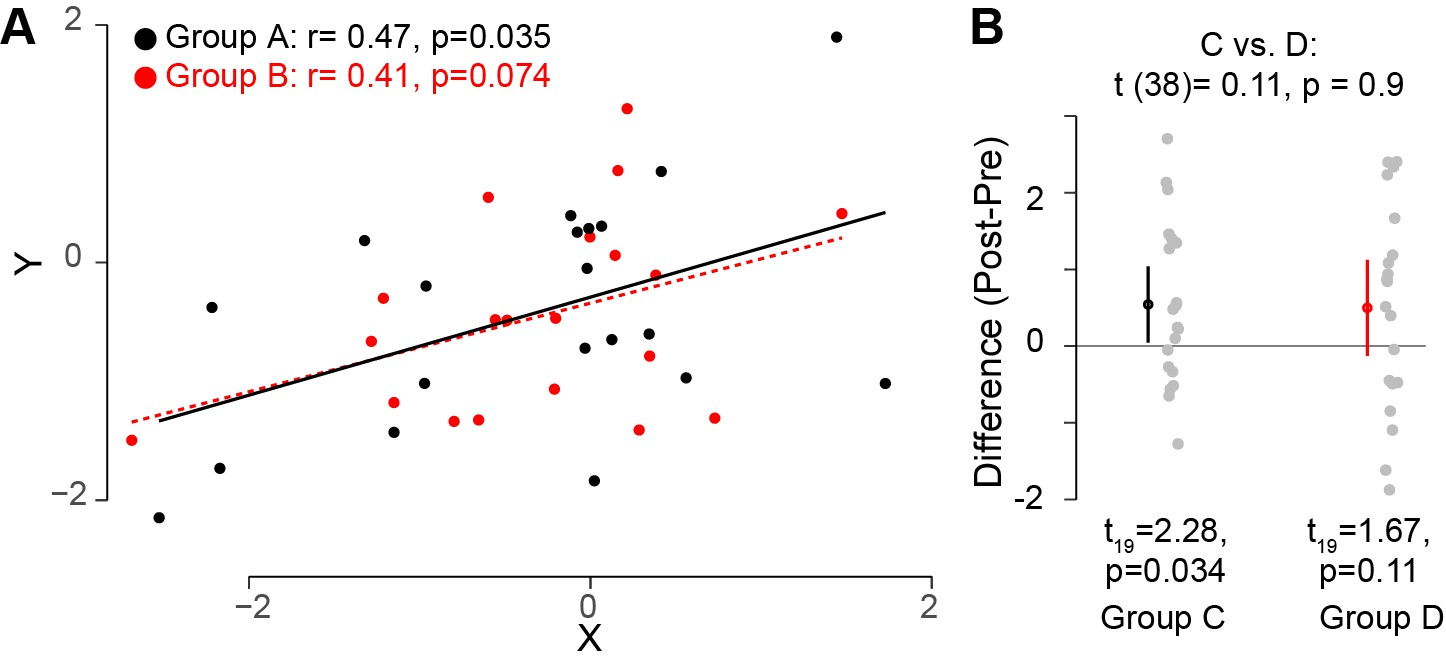
Interpreting comparisons between two effects without directly comparing them.
(A) Two variables, X and Y, were measured for two groups A and B. It looks clear that the correlation between these two variables does not differ across these two groups. However, if one compares both correlation coefficients to zero by calculating the significance of the Pearson's correlation coefficient r, it is possible to find that one group (group A; black circles; n = 20) has a statistically significant correlation (based on a threshold of p≤0.05), whereas the other group (group B, red circles; n = 20) does not. However, this does not indicate that the correlation between the variables X and Y differs between these groups. Monte Carlo simulations can be used to compare the correlations in the two groups (Wilcox and Tian, 2008). (B) In another experimental context, one can look at how a specific outcome measure (e.g. the difference pre- and post-training) differs between two groups. The means for groups C and D are the same, but the variance for group D is higher. If one uses a one-sample t-test to compare this outcome measure to zero for each group separately, it is possible to find that, this variable is significantly different from zero for one group (group C; left; n = 20), but not for the other group (group D, right; n = 20). However, this does not inform us whether this outcome measure is different between the two groups. Instead, one should directly compare the two groups by using an unpaired t-test (top): this shows that this outcome measure is not different for the two groups. Code (including the simulated data) available at github.com/jjodx/InferentialMistakes (Makin and Orban de Xivry, 2019; https://github.com/elifesciences-publications/InferentialMistakes).
A similar issue occurs when estimating the effect of an intervention measured in two different groups: the intervention could yield a significant effect in one group but not in the other (Figure 1B). Again, however, this does not mean that the effect of the intervention is different between the two groups; indeed in this case, the two groups do not significantly differ. One can only conclude that the effect of an intervention is different from the effect of a control intervention through a direct statistical comparison between the two effects. Therefore, rather than running two separate tests, it is essential to use one statistical test to compare the two effects.
How to detect it
This problem arises when a conclusion is drawn regarding a difference between two effects without statistically comparing them. This problem can occur in any situation where researchers make an inference without performing the necessary statistical analysis.
Solutions for researchers
Researchers should compare groups directly when they want to contrast them (and reviewers should point authors to Nieuwenhuis et al., 2011 for a clear explanation of the problem and its impact). The correlations in the two groups can be compared with Monte Carlo simulations (Wilcox and Tian, 2008). For group comparisons, ANOVA might be suitable. Although non-parametric statistics offers some tools (e.g., Leys and Schumann, 2010), these require more thought and customisation.
Further reading
Inflating the units of analysis
The problem
The experimental unit is the smallest observation that can be randomly and independently assigned, i.e. the number of independent values that are free to vary (Parsons et al., 2018). In classical statistics, this unit will reflect the degrees of freedom (df): For example, when inferring group results, the experimental unit is the number of subjects tested, rather than the number of observations made within each subject. But unfortunately, researchers tend to mix up these measures, resulting in both conceptual and practical issues. Conceptually, without clear identification of the appropriate unit to assess variation that sub-serves the phenomenon, the statistical inference is flawed. Practically, this results in a spuriously higher number of experimental units (e.g., the number of observations across all subjects is usually greater than the number of subjects). When df increases, the critical statistical threshold against which statistical significance is judged decreases, making it easier to observe a significant result if there is a genuine effect (increase of statistical power). This is because there is greater confidence in the outcome of the test.
To illustrate this issue, let us consider a simple pre-post longitudinal design for an intervention study in 10 participants where the researchers are interested in evaluating whether there is a correlation between their main measure and a clinical condition using a simple regression analysis. Their unit of analysis should be the number of data points (1 per participant, 10 in total), resulting in 8 df. For df = 8, the critical R value (with an alpha level of. 05) for achieving significance is 0.63. That is, any correlation above the critical value will be significant (p≤0.05). If the researchers combine the pre and post measures across participants, they will end up with df = 18, the critical R value is now 0.44, rendering it easier to observe a statistically significant effect. This is inappropriate because they are mixing within- and between- analysis units, resulting in dependencies between their measures – the pre-score of a given subject cannot be varied without impacting their post-score, meaning they only truly have 8 independent df. This often results in interpretation of the results as significant when in fact the evidence is insufficient to reject the possibility that there is no effect.
How detect it
The reviewer should consider the appropriate unit of analysis. If a study aims to understand group effects, then the unit of analysis should reflect the variance across subjects, not within subjects.
Solutions for researchers
Perhaps the best available solution to this issue is using a mixed-effects linear model, where researchers can define the variability within subjects as a fixed effect, and the between-subject variability as a random effect. This increasingly popular approach (Boisgontier and Cheval, 2016) allows one to put all the data in the model without violating the assumption of independence. However, it can be easily misused (Matuschek et al., 2017) and requires advanced statistical understanding, and as such should be applied and interpreted with some caution. For a simple regression analysis, the researchers have several available solutions to this issue, the easiest of which is to calculate the correlation for each observation separately (e.g. pre, post) and interpret the R values based on the existing df. The researchers can also average the values across observations, or calculate the correlation for pre/post separately and then average the resulting R values (after applying normalisation of the R distribution, e.g. r-to-Z transformation), and interpret them accordingly.
Further reading
Spurious correlations
The problem
Correlations are an important tool in science in order to assess the magnitude of an association between two variables. Yet, the use of parametric correlations, such as Pearson’s R relies on a set of assumptions, which are important to consider as violation of these assumptions may give rise to spurious correlations. Spurious correlations most commonly arise if one or several outliers are present for one of the two variables. As illustrated in the top row of Figure 2, a single value away from the rest of the distribution can inflate the correlation coefficient. Spurious correlations can also arise from clusters, e.g. if the data from two groups are pooled together when the two groups differ in those two variables (as illustrated in the bottom row of Figure 2).
Figure 2
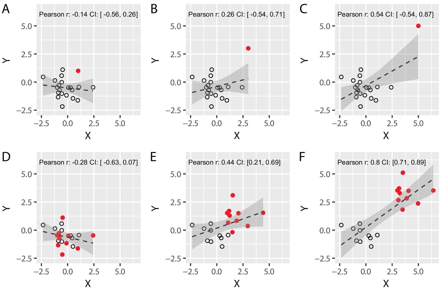
Spurious correlations: the effect of a single outlier and of subgroups on Pearson’s correlation coefficients.
(A–C) We simulated two different uncorrelated variables with 19 samples (black circles) and added an additional data point (solid red circle) whose distance from the main population was systematically varied until it became a formal outlier (panel C). Note that the value of Pearson’s correlation coefficient R artificially increases as the distance between the main population and the red data point is increased, demonstrating that a single data point can lead to spurious Pearson’s correlations. (D–F) We simulated two different uncorrelated variables with 20 sample that were arbitrarily divided into two subgroups (red vs. black, N = 10 each). We systematically varied the distance between the two subgroups from panel D to panel F. Again, the value of R artificially increases as the distance between the subgroups is increased. This shows that correlating variables without taking the existence of subgroups into account can yield spurious correlations. Confidence intervals (CI) are shown in grey, and were obtained via a bootstrap procedure (with the grey region representing the region between the 2.5 and 97.5 percentiles of the obtained distribution of correlation values). Code (including the simulated data) available at github.com/jjodx/InferentialMistakes.
It is important to note that an outlier might very well provide a genuine observation which obeys the law of the phenomenon that you are trying to discover, in other words – the observation in itself is not necessarily spurious. Therefore, removal of ‘extreme’ data points should also be considered with great caution. But if this true observation is at risk of violating the assumptions of your statistical test, it becomes spurious de facto, and will therefore require a different statistical tool.
How to detect it
Reviewers should pay particular attention to reported correlations that are not accompanied by a scatterplot and consider if sufficient justification has been provided when data points have been discarded. In addition, reviewers need to make sure that between-group or between-condition differences are taken into account if data are pooled together (see 'Inflating the units of analysis' above).
Solutions for researchers
Robust correlation methods (e.g. bootstrapping, data winsorizing, skipped correlations) should be preferred in most circumstances because they are less sensitive to outliers (Salibian-Barrera and Zamar, 2002). This is because these tests take into consideration the structure of the data (Wilcox, 2016). When using parametric statistics, data should be screened for violation of the key assumptions, such as independence of data points, as well as the presence of outliers.
Further reading
Use of small samples
The problem
When a sample size is small, one can only detect large effects, thereby leaving high uncertainty around the estimate of the true effect size and leading to an overestimation of the actual effect size (Button et al., 2013). In frequentist statistics in which a significance threshold of alpha=0.05 is used, 5% of all statistical tests will yield a significant result in the absence of an actual effect (false positives; Type I error). Yet, researchers are more likely to consider a correlation with a high coefficient (e.g. R>0.5) as robust than a modest correlation (e.g. R=0.2). With small sample sizes, the effect size of these false positives is large, giving rise to the significance fallacy: “If the effect size is that big with a small sample, it can only be true.” (This incorrect inference is noted in Button et al., 2013). Critically, the larger correlation is not a result of there being a stronger relationship between the two variables, it is simply because the overestimation of the actual correlation coefficient (here, R = 0) will always be larger with a small sample size. For instance, when sampling two uncorrelated variables with N = 15, simulated false-positive correlations roughly range between |0.5-0.75| whereas when sampling the same uncorrelated variables with N = 100 yields false-positive correlations in the range |0.2-0.25| (Code available at github.com/jjodx/InferentialMistakes).
Designs with a small sample size are also more susceptible to missing an effect that exists in the data (Type II error). For a given effect size (e.g., the difference between two groups), the chances are greater for detecting the effect with a larger sample size (this likelihood is referred to as statistical power). Hence, with large samples, you reduced the likelihood of not detecting an effect when one is actually present.
Another problem related to small sample size is that the distribution of the sample is more likely to deviate from normality, and the limited sample size makes it often impossible to rigorously test the assumption of normality (Ghasemi and Zahediasl, 2012). In regression analysis, deviations from the distribution might produce extreme outliers, resulting in spurious significant correlations (see 'Spurious correlations' above).
How to detect it
Reviewers should critically examine the sample size used in a paper and, judge whether the sample size is sufficient. Extraordinary claims based on a limited number of participants should be flagged in particular.
Solutions for researchers
A single effect size or a single p-value from a small sample is of limited value and reviewers can refer the researchers to Button et al. (2013) to make this point. The researchers should either present evidence that they have been sufficiently powered to detect the effect to begin with, such as through the presentation of an a priori statistical power analysis, or perform a replication of their study. The challenge with power calculations is that these should be based on an a priori calculation of effect size from an independent dataset, and these are difficult to assess in a review. Bayesian statistics offer opportunities to determine the power for identifying an effect post hoc (Kruschke, 2011). In situations where sample size may be inherently limited (e.g. research with rare clinical populations or non-human primates), efforts should be made to provide replications (both within and between cases) and to include sufficient controls (e.g. to establish confidence intervals). Some statistical solutions are offered for assessing case studies (e.g., the Crawford t-test; Corballis, 2009).
Further reading
Circular analysis
The problem
Circular analysis is any form of analysis that retrospectively selects features of the data to characterise the dependent variables, resulting in a distortion of the resulting statistical test (Kriegeskorte et al., 2010). Circular analysis can take many shapes and forms, but it inherently relates to recycling the same data to first characterise the test variables and then to make statistical inferences from them, and is thus often referred to as ‘double dipping’ (Kriegeskorte et al., 2009). Most commonly, circular analysis is used to divide (e.g. sub-grouping, binning) or reduce (e.g. defining a region of interest, removing ‘outliers’) the complete dataset using a selection criterion that is retrospective and inherently relevant to the statistical outcome.
For example, let’s consider a study of a neuronal population firing rate in response to a given manipulation. When comparing the population as a whole, no significant differences are found between pre and post manipulation. However, the researchers observe that some of the neurons respond to the manipulation by increasing their firing rate, whereas others decrease in response to the manipulation. They therefore split the population to sub-groups, by binning the data based on the activity levels observed at baseline. This leads to a significant interaction effect – those neurons that initially produced low responses show response increases, whereas the neurons that initially showed relatively increased activity exhibit reduced activity following the manipulation. However, this significant interaction is a result of the distorting selection criterion and a combination of statistical artefacts (regression to the mean, floor/ceiling effects), and could therefore be observed in pure noise (Holmes, 2009).
Another common form of circular analysis is when dependencies are created between the dependent and independent variables. Continuing with the example from above, researchers might report a correlation between the cell response post-manipulation and between the difference in cell response across the pre- and post-manipulation. But both variables are highly dependent on the post-manipulation measure. Therefore, neurons that by chance fire more strongly in the post manipulation measure are likely to show greater changes relative to the independent pre-manipulation measure, thus inflating the correlation (Holmes, 2009).
Selective analysis is perfectly justifiable when the results are statistically independent of the selection criterion under the null hypothesis. However, circular analysis recruits the noise (inherent to any empirical data) to inflate the statistical outcome, resulting in distorted and hence invalid statistical inference.
How to detect it
Circular analysis manifests in many different forms, but in principle occurs whenever the statistical test measures are biased by the selection criteria in favour of the hypothesis being tested. In some circumstances this is very clear, e.g. if the analysis is based on data that were selected for showing the effect of interest, or an inherently related effect. In other circumstances the analysis could be convoluted and require more nuanced understanding of co-dependencies across selection and analysis steps (see, for example, Figure 1 in Kilner, 2013 and the supplementary materials in Kriegeskorte et al., 2009). Reviewers should be alerted by impossibly high effect sizes which might not be theoretically plausible, and/or are based on relatively unreliable measures (if two measures have poor internal consistency this limits the potential to identify a meaningful correlation; Vul et al., 2009). In that case, the reviewers should ask the authors for a justification for the independence between the selection criteria and the effect of interest.
Solutions for researchers
Defining the analysis criteria in advance and independently of the data will protect researchers from circular analysis. Alternatively, since circular analysis works by ‘recruiting’ noise to inflate the desired effect, the most straightforward solution is to use a different dataset (or different part of your dataset) for specifying the parameters for the analysis (e.g. selecting your sub-groups) and for testing your predictions (e.g. examining differences across the sub-groups). This division can be done at the participant level (using a different group to identify the criteria for reducing the data) or at the trial level (using different trials but from all participants). This can be achieved without losing statistical power using bootstrapping approaches (Curran-Everett, 2009). If suitable, the reviewer could ask the authors to run a simulation to demonstrate that the result of interest is not tied to the noise distribution and the selection criteria.
Further reading
Flexibility of analysis: p-hacking
The problem
Using flexibility in data analysis (such as switched outcome parameters, adding covariates, undetermined or erratic pre-processing pipeline, post hoc outlier or subject exclusion; Wicherts et al., 2016) increases the probability of obtaining significant p-values (Simmons et al., 2011). This is because normative statistics rely on probabilities and therefore the more tests you run the more likely you are to encounter a false positive result. Therefore, observing a significant p-value in a given dataset is not necessarily complicated and one can always come up with a plausible explanation for any significant effect particularly in the absence of specific predictions. Yet, the more variation in one’s analysis pipeline, the greater the likelihood that observed effects are not genuine. Flexibility in data analysis is especially visible when the same community reports the same outcome variable but computes the value of this variable in different ways across the paper (e.g. www.flexiblemeasures.com; Carp, 2012; Francis, 2013) or when clinical trials switch their outcomes (Altman et al., 2017; Goldacre et al., 2019).
This problem can be pre-empted by using standardised analytic approaches, pre-registration of the design and analysis (Nosek and Lakens, 2014), or undertaking a replication study (Button et al., 2013). Note that pre-registration of experiments can be performed after the results of a first experiment are known and before an internal replication of that effect is sought. But perhaps the best way to prevent p-hacking is to show some tolerance to borderline or non-significant results. In other words, if the experiment is well designed, executed, and analysed, reviewers should not 'punish' the researchers for their data.
How to detect it
Flexibility of analysis is difficult to detect because researchers rarely disclose all the necessary information. In the case of pre-registration or clinical trial registration, the reviewer should compare the analyses performed with the planned analyses. In the absence of pre-registration, it is almost impossible to detect some forms of p-hacking. Yet, reviewers can estimate whether all the analysis choices are well justified, whether the same analysis plan was used in previous publications, whether the researchers came up with a questionable new variable, or whether they collected a large battery of measures and only reported a few significant ones. Practical tips for detecting likely positive findings are summarized in Forstmeier et al. (2017).
Solutions for researchers
Researchers should be transparent in the reporting of the results, e.g. distinguishing pre-planned versus exploratory analyses and predicted versus unexpected results. As we discuss below, exploratory analyses using flexible data analysis are fine if they are reported and interpreted as such in a transparent manner and especially so if they serve as the basis for a replication with pre-specified analyses (Curran-Everett and Milgrom, 2013). Such analyses can be a valuable justification for additional research but cannot be the foundation for strong conclusions.
Further reading
Failing to correct for multiple comparisons
The problem
When researchers explore task effects, they often explore the effect of multiple task conditions on multiple variables (behavioural outcomes, questionnaire items, etc.), sometimes with an underdetermined a priori hypothesis. This practice is termed exploratory analysis, as opposed to confirmatory analysis, which by definition is more restrictive. When performed with frequentist statistics, conducting multiple comparisons during exploratory analysis can have profound consequences for the interpretation of significant findings. In any experimental design involving more than two conditions (or a comparison of two groups), exploratory analysis will involve multiple comparisons and will increase the probability of detecting an effect even if no such effect exists (false positive, type I error). In this case, the larger the number of factors, the greater the number of tests that can be performed. As a result, the probability of observing a false-positive increases (family-wise error rate). For example, in a 2 × 3 × 3 experimental design the probability of finding at least one significant main or interaction effect is 30%, even when there is no effect (Cramer et al., 2016).
This problem is particularly salient when conducting multiple independent comparisons (e.g. neuroimaging analysis, multiple recorded cells or EEG). In such cases, researchers are technically deploying statistical tests within every voxel/cell/timepoint, thereby increasing the likelihood of detecting a false positive result, due to the large number of measures included in the design. For example, Bennett and colleagues (Bennett et al., 2009) identified a significant number of active voxels in a dead Atlantic Salmon (activated during a 'mentalising' task) when not correcting for multiple comparisons. This example demonstrates how easy it can be to identify a spurious significant result. Although it is more problematic when the analyses are exploratory, it can still be a concern when a large set of analyses are specified a priori for confirmatory analysis.
How to detect it
Failing to correct for multiple comparisons can be detected by addressing the number of independent variables measured and the number of analyses performed. If only one of these variables correlated with the dependent variable, then the rest is likely to have been included to increase the chance of obtaining a significant result. Therefore, when conducting exploratory analyses with a large set of variables (such as genes or MRI voxels), it is simply unacceptable for the researchers to interpret results that have not survived correction for multiple comparisons, without clear justification. Even if the researchers offer a rough prediction (e.g. that the effect should be observed in a specific brain area or at an approximate latency), if this prediction could be tested over multiple independent comparisons, it requires correction for multiple comparisons.
Solutions for researchers
Exploratory testing can be absolutely appropriate, but should be acknowledged. Researchers should disclose all measured variables and properly implement the use of multiple comparison procedures. For example, applying standard corrections for multiple comparisons unsurprisingly resulted in no active voxels in the dead fish example (Bennett et al., 2009). Bear in mind that there are many ways to correct for multiple comparisons, some more well accepted than others (Eklund et al., 2016), and therefore the mere presence of some form of correction may not be sufficient.
Further reading
Over-interpreting non-significant results
The problem
When using frequentist statistics, scientists apply a statistical threshold (normally alpha=.05) for adjudicating statistical significance. Much has been written about the arbitrariness of this threshold (Wasserstein et al., 2019) and alternatives have been proposed (e.g., Colquhoun, 2014; Lakens et al., 2018; Benjamin et al., 2018). Aside from these issues, which we elaborate on in our final remarks, misinterpreting the results of a statistical test when the outcome is not significant is also highly problematic but extremely common. This is because a non-significant p-value does not distinguish between the lack of an effect due to the effect being objectively absent (contradictory evidence to the hypothesis) or due to the insensitivity of the data to enable to the researchers to rigorously evaluate the prediction (e.g. due to lack of statistical power, inappropriate experimental design, etc.). In simple words - non-significant effects could literally mean very different things - a true null result, an underpowered genuine effect, or an ambiguous effect (see Altman and Bland, 1995 for an example). Therefore, if the researchers wish to interpret a non-significant result as supporting evidence against the hypothesis, they need to demonstrate that this evidence is meaningful. The p-value in itself is insufficient for this purpose. This confound also means that sometimes researchers might ignore a result that did not meet the p≤0.05 threshold, assuming it is meaningless when in fact it provides sufficient evidence against the hypothesis or at least preliminary evidence that requires further attention.
How to detect it
Researchers might interpret or describe a non-significant p-value as indicating that an effect was not present. This error is very common and should be highlighted as problematic.
Solutions for researchers
An important first step is to report effect sizes together with p-values in order to provide information about the magnitude of the effect (Sullivan and Feinn, 2012), which is also important for any future meta-analyses (Lakens, 2013; Weissgerber et al., 2018). For example, if a non-significant effect in a study with a large sample size is also very small in magnitude, it is unlikely to be theoretically meaningful whereas one with a moderate effect size could potentially warrant further research (Fethney, 2010). When possible, researchers should consider using statistical approaches that are capable of distinguishing between insufficient (or ambiguous) evidence and evidence that supports the null hypothesis (e.g., Bayesian statistics; [Dienes, 2014], or equivalence tests [Lakens, 2017]). Alternatively, researchers might have already determined a priori whether they have sufficient statistical power to identify the desired effect, or to determine whether the confidence intervals of this prior effect contain the null (Dienes, 2014). Otherwise, researchers should not over-interpret non-significant results and only describe them as non-significant.
Further reading
(Dienes, 2014).
Correlation and causation
The problem
This is perhaps the oldest and most common error made when interpreting statistical results (see, for example, Schellenberg, 2019). In science, correlations are often used to explore the relationship between two variables. When two variables are found to be significantly correlated, it is often tempting to assume that one causes the other. This is, however, incorrect. Just because variability of two variables seems to linearly co-occur does not necessarily mean that there is a causal relationship between them, even if such an association is plausible. For example, a significant correlation observed between annual chocolate consumption and number of Nobel laureates for different countries (r(20)=.79; p<0.001) has led to the (incorrect) suggestion that chocolate intake provides nutritional ground for sprouting Nobel laureates (Maurage et al., 2013). Correlation alone cannot be used as an evidence for a cause-effect relationship. Correlated occurrences may reflect direct or reverse causation, but can also be due to an (unknown) common cause, or they may be a result of a simple coincidence.
How to detect it
Whenever the researcher reports an association between two or more variables that is not due to a manipulation and uses causal language, they are most likely confusing correlation and causation. Researchers should only use causal language when a variable is precisely manipulated and even then, they should be cautious about the role of third variables or confounding factors.
Solutions for researchers
If possible, the researchers should try to explore the relationship with a third variable to provide further support for their interpretation, e.g. using hierarchical modelling or mediation analysis (but only if they have sufficient power), by testing competing models or by directly manipulating the variable of interest in a randomised controlled trial (Pearl, 2009). Otherwise, causal language should be avoided when the evidence is correlational.
Further reading
(Pearl, 2009).
Final remarks
Avoiding these ten inference errors is an important first step in ensuring that results are not grossly misinterpreted. However, a key assumption that underlies this list is that significance testing (as indicated by the p-value) is meaningful for scientific inferences. In particular, with the exception of a few items (see 'Absence of an adequate control condition/group' and 'Correlation and causation'), most of the issues we raised, and the solution we offered, are inherently linked to the p-value, and the notion that the p-value associated with a given statistical test represents its actual error rate. There is currently an ongoing debate about the validity of null-hypothesis significance testing and the use of significance thresholds (Wasserstein et al., 2019). We agree that no single p-value can reveal the plausibility, presence, truth, or importance of an association or effect. However, banning p-values does not necessarily protect researchers from making incorrect inferences about their findings (Fricker et al., 2019). When applied responsibly (Kmetz, 2019; Krueger and Heck, 2019; Lakens, 2019), p-values can provide a valuable description of the results, which at present can aid scientific communication (Calin-Jageman and Cumming, 2019), at least until a new consensus for interpreting statistical effects is established. We hope that this paper will help authors and reviewers with some of these mainstream issues.
Further reading
Data availability
Simulated data and code used to generate the figures in the commentary are available online.
References
-
Redefine statistical significanceNature Human Behaviour 2:6–10.https://doi.org/10.1038/s41562-017-0189-z
-
The principled control of false positives in neuroimagingSocial Cognitive and Affective Neuroscience 4:417–422.https://doi.org/10.1093/scan/nsp053
-
The anova to mixed model transitionNeuroscience & Biobehavioral Reviews 68:1004–1005.https://doi.org/10.1016/j.neubiorev.2016.05.034
-
Power failure: Why small sample size undermines the reliability of neuroscienceNature Reviews Neuroscience 14:365–376.https://doi.org/10.1038/nrn3475
-
The new statistics for better science: Ask how much, how uncertain, and what else is knownThe American Statistician 73:271–280.https://doi.org/10.1080/00031305.2018.1518266
-
An investigation of the false discovery rate and the misinterpretation of p-valuesRoyal Society Open Science 1:140216.https://doi.org/10.1098/rsos.140216
-
Hidden multiplicity in exploratory multiway ANOVA: Prevalence and remediesPsychonomic Bulletin & Review 23:640–647.https://doi.org/10.3758/s13423-015-0913-5
-
Explorations in statistics: The bootstrapAdvances in Physiology Education 33:286–292.https://doi.org/10.1152/advan.00062.2009
-
Post-hoc data analysis: benefits and limitationsCurrent Opinion in Allergy and Clinical Immunology 13:223–224.https://doi.org/10.1097/ACI.0b013e3283609831
-
Bayesian versus orthodox statistics: Which side are you on?Perspectives on Psychological Science 6:274–290.https://doi.org/10.1177/1745691611406920
-
Using Bayes to get the most out of non-significant resultsFrontiers in Psychology 5:781.https://doi.org/10.3389/fpsyg.2014.00781
-
Detecting and avoiding likely false-positive findings - a practical guideBiological Reviews 92:1941–1968.https://doi.org/10.1111/brv.12315
-
Replication, statistical consistency, and publication biasJournal of Mathematical Psychology 57:153–169.https://doi.org/10.1016/j.jmp.2013.02.003
-
Normality tests for statistical analysis: A guide for non-statisticiansInternational Journal of Endocrinology and Metabolism 10:486–489.https://doi.org/10.5812/ijem.3505
-
The annual cannabis holiday and fatal traffic crashesInjury Prevention 25:433–437.https://doi.org/10.1136/injuryprev-2018-043068
-
HARKing: Hypothesizing after the results are knownPersonality and Social Psychology Review 2:196–217.https://doi.org/10.1207/s15327957pspr0203_4
-
Bias in a common EEG and MEG statistical analysis and how to avoid itClinical Neurophysiology 124:2062–2063.https://doi.org/10.1016/j.clinph.2013.03.024
-
Correcting corrupt research: Recommendations for the profession to stop misuse of p-valuesThe American Statistician 73:36–45.https://doi.org/10.1080/00031305.2018.1518271
-
Why is the one-group pretest-posttest design still used?Clinical Nursing Research 25:467–472.https://doi.org/10.1177/1054773816666280
-
Circular analysis in systems neuroscience: The dangers of double dippingNature Neuroscience 12:535–540.https://doi.org/10.1038/nn.2303
-
Everything you never wanted to know about circular analysis, but were afraid to askJournal of Cerebral Blood Flow & Metabolism 30:1551–1557.https://doi.org/10.1038/jcbfm.2010.86
-
Putting the p-value in its placeAmerican Statistician 73:122–128.https://doi.org/10.1080/00031305.2018.1470033
-
Bayesian assessment of null values via parameter estimation and model comparisonPerspectives on Psychological Science 6:299–312.https://doi.org/10.1177/1745691611406925
-
Equivalence tests: A practical primer for t tests, correlations, and meta-analysesSocial Psychological and Personality Science 8:355–362.https://doi.org/10.1177/1948550617697177
-
A nonparametric method to analyze interactions: The adjusted rank transform testJournal of Experimental Social Psychology 46:684–688.https://doi.org/10.1016/j.jesp.2010.02.007
-
Balancing type I error and power in linear mixed modelsJournal of Memory and Language 94:305–315.https://doi.org/10.1016/j.jml.2017.01.001
-
A manifesto for reproducible scienceNature Human Behaviour 1:0021.https://doi.org/10.1038/s41562-016-0021
-
Erroneous analyses of interactions in neuroscience: A problem of significanceNature Neuroscience 14:1105–1107.https://doi.org/10.1038/nn.2886
-
How does multiple testing correction work?Nature Biotechnology 27:1135–1137.https://doi.org/10.1038/nbt1209-1135
-
Causal inference in statistics: An overviewStatistics Surveys 3:96–146.https://doi.org/10.1214/09-SS057
-
Improving standards in brain-behavior correlation analysesFrontiers in Human Neuroscience 6:119.https://doi.org/10.3389/fnhum.2012.00119
-
Bootrapping robust estimates of regressionThe Annals of Statistics 30:556–582.https://doi.org/10.1214/aos/1021379865
-
Correlation = causation? Music training, psychology, and neurosciencePsychology of Aesthetics, Creativity, and the Arts.https://doi.org/10.1037/aca0000263
-
What errors do peer reviewers detect, and does training improve their ability to detect them?Journal of the Royal Society of Medicine 101:507–514.https://doi.org/10.1258/jrsm.2008.080062
-
Using effect size - or why the p value is not enoughJournal of Graduate Medical Education 4:279–282.https://doi.org/10.4300/JGME-D-12-00156.1
-
ANCOVA versus change from baseline had more power in randomized studies and more bias in nonrandomized studiesJournal of Clinical Epidemiology 59:920–925.https://doi.org/10.1016/j.jclinepi.2006.02.007
-
Puzzlingly high correlations in fMRI studies of emotion, personality, and social cognitionPerspectives on Psychological Science 4:274–290.https://doi.org/10.1111/j.1745-6924.2009.01125.x
-
Moving to a world beyond “p < 0.05”The American Statistician 73:1–19.https://doi.org/10.1080/00031305.2019.1583913
-
Comparing dependent robust correlationsBritish Journal of Mathematical and Statistical Psychology 69:215–224.https://doi.org/10.1111/bmsp.12069
-
Comparing dependent correlationsThe Journal of General Psychology 135:105–112.https://doi.org/10.3200/GENP.135.1.105-112
Decision letter
-
Peter RodgersSenior and Reviewing Editor; eLife, United Kingdom
-
Nick ParsonsReviewer; University of Warwick, Coventry, United Kingdom
-
Nick HolmesReviewer; University of Nottingham, Nottingham, United Kingdom
In the interests of transparency, eLife includes the editorial decision letter and accompanying author responses. A lightly edited version of the letter sent to the authors after peer review is shown, indicating the most substantive concerns; minor comments are not usually included.
Thank you for submitting your article "Ten common inferential mistakes to watch out for when writing or reviewing a manuscript" to eLife for consideration as a Features Article. Your article has been reviewed by two peer reviewers, who have both agreed to reveal their identity: Nick Parsons; Nick Holmes.
Both reviewers produced very substantial reports, and rather than consolidate them as normally happens at eLife, I have combined them so that all the comments on each section of your article are together. This means that the decision letter is very long – and also somewhat critical in a few places – but both referees really engaged with the manuscript
I would like to invite you to submit a revised version of your article that addresses these comments. While the list of comments below is rather long, the reviewers and myself feel that it should be possible to address them within a reasonable time frame.
Also, please note the following:
1) Please remove section 6 (and consider replacing it with a section on 'circular analyses' – as suggested by the referees).
2) Please revise Figure 1 (see comments below).
3) Please remove Figure 3 and Figure 4.
Summary:
Reviewer #1:
Overall, I enjoyed reading this manuscript. It certainly has some merit.
However, at times I found myself profoundly disagreeing with some of the recommendations. I give a list of some of my more significant gripes below. I think this manuscript could be suitable for publication, but there needs to be a substantial amount of additional work to make it make it so.
First, I do not know the background of the authors (so apologies if I offend), but some of the wording and examples and description suggests that they are not themselves experienced applied statisticians. This manuscript would benefit enormously from the input of such a person, simply to reformulate some of the common mistakes and link in with well-known issues that statisticians typically observe when teaching statisticians, advising colleagues and reviewing manuscripts. I accept that it is important to have the tone and voice of the scientist (and not the statistician) in this manuscript, but it is important that the manuscript is such that it is has a much stronger statistical basis, to give it more weight.
Much of the text here is quite wordy and the explanations of the issues often confusing (e.g. issues 3 and 4). I am sure the authors could make these much simpler and easier to understand. The background of the authors is clearly in the neurosciences. This shows with their choice of examples at times (e.g. issue 1). This manuscript would work just as well with more neutral examples that would be understandable to anyone across the range of scientific disciplines. So, I suggest the authors re-write in such a way.
Manuscripts such as this are important and can have significant impact on not just the reporting of science, but also how it is done. So, I hope the authors decide to make appropriate changes to the manuscript in order to make it more acceptable for publication.
Essential revisions:
0) Introduction
Reviewer #1:
– It is worth making the point in the Introduction that many journals undertake in-house statistical reviews and/or send manuscripts out for more detailed statistical review if reviewers of the substantive content have concerns.
1) Absence of a control condition/group
Reviewer #1:
– This manuscript is at times very neuroscience focused. I understand that is the primary interest of the authors, but at times I think it simply distracts from the message and much simpler examples (that would be universal to all scientists) would have worked much better. That is particularly the case with this first common 'mistake'.
Reviewer #2:
– 'inflating the likelihood of observing spurious changes' – But all statistical tests are done using probabilities of false positives, which depend on the variability in the data. What is the evidence that low test-retest reliability leads to increased false-positive outcomes? As this section notes, it is only the absolute size of the difference that will be 'observed' – statistics will tell us if this difference is reliable or not, and that is where the (fixed) false-positive rate applies.
– I often come across control groups that are sampled after the results of the experimental group are known (e.g., lots of TMS studies). I would add here that control and experimental groups need to be sampled at the same time and with randomised allocation.
– This is not only 'longitudinal', this applies to cross-sectional data too.
2) Interpreting comparisons between two effects without directly comparing them
Reviewer #1:
– Figure 1 – This is an oddly chosen example. Clearly the variance in group B is much greater than the variance in group A. This explains (in part at least) why the test of the group differences is not significant. But, surely pooling here is problematic: we are assuming, for the methods suggested, that the variance is the same in each group whereas, to most, it looks like it is very different. The authors need to choose a better example to illustrate common mistake 2, and modify Figure 1 appropriately.
Reviewer #2:
– This problem applies also not just to 'difference scores' but any effect (e.g., a slope, curve-fit etc., not just 'differences'). I suggest the authors make it more general here (as they do in 'how to detect'), then give the specific and useful example of the simple difference of two differences. It may also be worth noting here that this is often the 'interaction' term in the analysis.
– 'differential statistical significance' – I would say something like 'different binary outcomes when applying a statistical threshold'.
3) Inflating degrees of freedom by violating independence of measures
Reviewer #1:
– This is a very complicated explanation for what most statisticians would describe in a very different way. It is needlessly complicated. This is what most statisticians would describe as the 'unit of analysis' issue – much described in the literature previously see e.g. Parsons, Teare and Sitch (2018, eLife).
Some poor practice is described here, where for example multiple measurements on the same subject are made as a means of ultimately comparing subjects. If a study aims to understand the effect of an intervention on subjects, then that is the 'unit of the analysis' and in order to draw inferences the replication must be at the level of the subject (the unit of analysis), not within subject (within unit). Multiple measurements on subjects improve the precision of estimation of the subject mean (for instance) but tell us nothing about the variability between subjects.
This is often observed as an artificial inflation of the degrees of freedom, pooling between strata in the analysis, but ultimately the problem is the lack of clear identification of the purpose of the analysis and the appropriate unit to use to assess variation that is used to quantify intervention effects. Personally, I don't think bringing correlation into the discussion helps a great deal. All we really need to be aware of is that measurements within (for instance) a subject are likely to be correlated, whereas by definition data from subjects are uncorrelated.
– Mixed-effects analysis – This is the canonical analysis that most statisticians would recommend. When we do this, we naturally estimate the appropriate within subject (cluster) correlations. This methodology should be much more widely used in many areas of science; only in medicine, where studies report patient data, and psychology is it generally recognised as being important. Although its roots go back to the genesis of statistics in agricultural science, where fields were divided into blocks, plots and nested sub-plots and plants etc.
– A priori statistical power analyses are always a good idea, but I really don't think it adds much to the discussion here.
Reviewer #2:
– This is true in some statistical procedures (e.g., where you model a single parameter at a single level for each participant), but not all. For example, I believe linear mixed models (e.g., in R), will have many dfs larger than N-x, yet these remain valid. I remember seeing large dfs in (e.g.) Brain Voyager FMRI outputs. I do not understand these multi-level linear mixed models, but I have questioned and been corrected on this df point by statisticians using R (e.g., see the df in Meteyard and Holmes, 2018; I didn't do the analysis). The recommendation in 'how to detect' should be clarified and/or corrected as necessary.
– 'average the resulting r values (don't forget to normalise the distribution first!)' – Perhaps give specific advice here: e.g., use Fisher's r-to-Z transformation, Z=0.5log[(1+r)/(1-r)]
– 'random factor' – 'random 'effect' would be better
4) Spurious correlations
Reviewer #1:
– Figure 2A, B, C – Surely the issue here is that 'outliers' have a big impact (leverage) on many statistics; means, variances, covariances, regression analyses, ANOVA and yes, correlations. But this is not an issue only of concern when estimating correlations. Surely the issue here is to present data visually and consider the meaning (validity) of any data points that are a long way from the rest of the distribution. I don't like the (implicit) argument here that the Pearson correlations are in some sense 'wrong'. It depends on whether the model is correct (straight line) and whether the assumptions of approximately normality are correct. It is perfectly plausible to believe Figure 2C is correct, and that only one data point was available at X=5, but there is good reason to believe that data are normally distributed. The point I would make here is the importance of error measurements when reporting. The confidence intervals of the Pearson correlation would help us enormously here. Point estimates of correlations alone are not that useful, unless the data are shown visually.
– The other thing I would take issue with here is the implication that Spearman's rank correlation makes more sense in settings Figure 2B and Figure 2C. In general, decisions about whether to assume normality are better made for principled reasons rather than for empirical reasons. Using a non-parametric correlation coefficient would make little sense to me here – they are generally very inefficient, as we convert to ranks first, which is the reason the value does not change from Figure 2B to Figure 2C. If data were reasonably tightly distributed symmetrically about the mean, other than one value which was a big distance away, my first recommendation would be to examine the credence of the extreme data point, not proceed to a non-parametric correlation.
Reviewer #2:
– 'Yet, the use of parametric correlations, such as Pearson's r, requires that both variables are normally distributed.'
No, it doesn't! All parametric linear models (as far as I understand) require that the error is normally distributed. In the case of a single-sample t-test against a single mean, this is identical to the requirement that the variables themselves are normally distributed. But, for everything else, it is the differences or error or residuals after the model is fit which must be normally distributed, not the raw data. The authors repeat in their tutorial what I understand to be a very common mis-interpretation, and it would be good for them to make absolutely certain that what they say here is correct, to avoid perpetuating these errors.
Here is a tutorial from the R team: https://rcompanion.org/handbook/I_01.html, specifically: "In particular, the tests discussed in this section assume that the distribution of the data are conditionally normal in distribution. That is, the data are normally distributed once the effects of the variables in the model are taken into account. Practically speaking, this means that the residuals from the analysis should be normally distributed. This will usually be assessed with a histogram of residuals, a density plot as shown below, or with a quantile-quantile plot… Be careful not to get confused about this assumption. You may see discussion about how "data" should be normally distributed for parametric tests. This is usually wrong-headed."
The authors are correct here that (genuine) outliers can lead to spurious correlations, but the remedy for this is, as they state: (a) plot the data, (b) run some robustness-checks, and to report all the results with their standard errors and with due caution.
One real problem is how do we identify 'genuine' outliers? Perhaps a large sample size is one remedy, so that we have a better coverage of the population? Yet, there will still be cases when clear 'outliers' are genuine observations which obey the law that you are trying to discover. For example, measuring mass vs. body length across the animal kingdom: there will be an awful lot of small animals down the bottom of the scale (e.g., insects), some in the middle (e.g., birds and most mammals), and fewer still at the extremes (e.g., whales or elephants). I would bet that the blue whale follows the same statistical law of mass vs. length as the gnat (with variance away from this model due to shape). A 'spurious' correlation might arise from incomplete sampling of the problem space – if we only sampled insects and whales, we might draw the wrong conclusion and call the correlation between mass and length 'spurious'. Or perhaps the data need log-transforming first?
My laboured point here is: if you don't have any independent reason to exclude a particular datapoint (e.g., the participant didn't do the task properly, wasn't wearing their glasses, is not healthy, is not typical; the elephant was stretching its legs), then I think it is dangerous to conclude that the correlation is spurious just because of one 'outlier'. Rather, authors need to present the data, check their assumptions, and speculate that sampling bias or experimenter error has led to this 'outlier'. In general, the authors are correct here: limited sampling of the intended population may make such outliers more likely, and correlations may then be more problematic. But this is all relative, and error can occur in both directions (Type I, Type II). The only solution is to be very careful, both in including and excluding data.
– 'when the two variables are not independent' – Repeated measures designs will often have highly-correlated scores between different conditions or time-points in the same participants. Again, is the real issue here 'independent error' (residuals) not 'independent data'?
– This is the 'regression towards the mean' error that I discussed in Holmes, (2007, 2009), yet this topic is only an "Honorable mention" here! I would suggest all these 'circular analyses' and 'double-dips' (i.e., both are experimenter-created dependencies in the data) could be in their own section (after dealing with the below comments, in which I suggest removing point 6 entirely).
– Figure 2A – I would bet that the red point is not an outlier here, as claimed in the legend.
– 'they can run some basic simulations' – I agree 100% (Holmes 2007, 2009), but this sentence will have, in my view, about 95% of your target audience hiding under the bedcovers in fear of programming. How does someone who is not sufficiently well-trained to spot these problems in the first place go about 'running some simulations'? Can the authors point to an online tool or tutorial that helps?
5) Use of underpowered groups
Reviewer #1:
– Experiments with small samples sizes are quite often small for very good reasons, not always but often. We should not recommend that scientists don't do small experiments – sometimes there is no option – but we should tell them not to report inferential statistics. Particularly if the study does not have an a priori power calculation. Not sure that Figure 3 adds much here.
Reviewer #2:
– 'In frequentist statistics in which a significance threshold of α=.05 is used, 5% of all statistical tests will yield a significant result even in the absence of an actual effect (false positives; Type I error)' – I think the authors need to clarify this a bit more, to, e.g.: "Assuming that the null is true, then randomly- and independently-sampled data from a normal distribution with a mean of zero will yield a sample that, when tested against a mean of zero, has a p-value below or equal to. 05 approximately 5% of the time." The word 'even' in their claim here is unhelpful – the stats explicitly assume that the null is true (it is never actually true!)
– 'Given that these two variables are random, there should be no significant correlations' – See previous point. There will be 5% 'significant' correlations.
– 'falsely significant' – I don't like this phrase. It seems contradictory. I know what they mean (something like: 'using the standard α criterion, most researchers would conclude that there is a positive correlation in the population when in fact there isn't').
– 'the experiment is underpowered' – But there is no effect in the simulated population. There can therefore be no sample size sufficient to find this effect. This cannot, therefore, be 'underpowered'. Revise.
– '<' should this, in fact, be '≤'? Same throughout the manuscript.
– 'Designs with a small sample size are also more susceptible to Type II errors' – Why? Type II error is a non-linear function of the sample size and the real effect size. Knowing the Type II error requires that you know the population distribution, which is almost never the case (and not required) in the kinds of parametric null-hypothesis tests that the authors are discussing here.
– 'based on a limited number of participants' – I would remove this as I don't think this it is justifiable. I think all effects (especially surprising ones) from a single experiment should be taken with the same degree of caution, regardless of their sample size (who sets the criterion in any case?). The statistics deal with the problem of sample size. Statistics can be biased as a function of sample size, of course, and some come with corrections (e.g., Hedges G instead of Cohen's d) but if you expect a large effect (e.g., removing striate cortex will impair vision), then I see nothing wrong with doing the absolute minimum of testing on your subjects to establish that effect. It would be unethical to remove 30 monkeys' visual cortices when 2 are sufficient to test the hypothesis.
– 'that were not replicated' – Yes, we should be especially skeptical if a second well-powered experiment failed to replicate the first, but I would only be normally skeptical of a single-experiment finding, regardless of its sample size. I think the authors' main point is that small studies will achieve significance only with large effects. True. But some large effects are real, so given a single particular result, how do you know? We must be allowed to search for large statistical effects. Collecting converging and independent evidences should be sought in all investigations, not just in those researchers looking for large effects: Smith and Little (2018).
6) Using parametric statistics with small sample sizes
Reviewer #1:
– Sorry but I cannot agree with much of this section. See my previous comments about normality assumptions. Tests of normality are really not very useful in most circumstances. In small samples, I agree with authors, they are useless. However, in large samples they will always reject with probability of very near one.
– In general, decisions about normality and whether to use parametric or non-parametric methods should be based mainly on scientific principle. For instance, if I collect data on the heights of 10 people, I report a median and IQR, but if I collect data on 50 people a mean and SD? No, that is clearly wrong. I believe that heights are approximately distributed, based on the way it is measured, my own experience and the experience of others (irrespective of what a test of normality tells me!), so I should summarise data on that basis in the appropriate way by a mean and SD.
– This sort of mechanical/automated approach to the implementation of statistical methods is strongly discouraged by the majority of statisticians. This is analogous to the widespread adherence to the (mis-) interpretation of p-values that has been so widely criticized by among others the American Statistical Association. In its guidance for the use of statistical tests for such decisions and the role of p-values it makes clear that "Scientific conclusions and business or policy decisions should not be based only on whether a p-value passes a specific threshold" and "No single index [the p-value] should substitute for scientific reasoning".
– Scientific reasoning and precedent should be used to make decisions about how to appropriately analyse data, not arbitrary ad hoc (data dependent) statistical tests.
Reviewer #2:
– Section 6 is incorrect and should be removed. In part, due to the same problem as point #4 (normal distribution of error), but, what the authors seem to be arguing for (unwittingly) is an abandonment of parametric tests, not for their use only with 'large' samples, as explained below:
Parametric statistics were designed for small samples. If in any doubt about this, please check out Fisher (1925), available in full here: https://psychclassics.yorku.ca/Fisher/Methods/index.htm
In parametric statistics, from a sample of data we extract parameters, for example the mean and the SD (e.g., of the difference between means of two conditions). In our statistical model we compare those parameters to a normal distribution in order to make probabilistic inferences using the theoretical distribution.
When sample size is small (say <30), we do not refer our parameters directly to the normal distribution. Rather, we refer them to the t, F, Chi-Square, Poisson, Binomial, or any other appropriate statistical distribution. These distributions were originally created by sampling small numbers of datapoints, and seeing how they behaved. These distributions are all skewed in interesting ways, but as N increases, they tend to approximate the normal distribution.
The (in my view) often-mistaken 'rule of thumb' that you need at least 30 participants to do parametric statistics is wrong. It is in my understanding, opposite this. As N increases, the t-, F, Binomial, Chi-square, and Poisson distributions converge closer and closer to the normal distribution. So, when N=30, rather than using the t-test, you can just use the Z-test (i.e., essentially ignoring sample size). The critical t-value for 1 degree of freedom (N=2) at α=.05 is 6.31 (i.e., 6.31 standard errors of your sample mean difference away from zero). As N increases to infinity, the critical value converges to 1.645. At N=30, the critical t-value is 1.7, which is arguably close-enough to the population Z-score (1.645) that the t-distribution can be abandoned (i.e., only sample size is relevant for calculating the SE, df is not needed) and that the Z-distribution can be used instead. Small samples are already 'punished' via the df, by requiring much larger effect sizes to pass arbitrary statistical thresholds.
My understanding is that most statistical tests are designed for small samples. Non-parametric tests are for non-interval and non-ratio data (categorical, ordinal), or for interval/ratio data with populations for which no reasonable assumptions can be made (e.g., with large inexplicable outliers). Bootstrapping or other non-parametric statistical methods can be useful to check whether small samples are indeed sufficiently normal to use parametric tests (e.g., from Makin et al., 2009, where Ns=6-11: "In every case, this bootstrapping procedure supported the inferences derived from the t tests, so we report only the standard parametric tests in this manuscript.").
As the authors correctly note, small samples come with biases (e.g., effect sizes are larger for significant effects), but this does not invalidate the use of parametric tests. The authors cite Kar and Ramalingam (2013) in support of their claim, yet from that paper's conclusion: "Hence, there is no such thing as a magic number when it comes to sample size calculations and arbitrary numbers such as 30 must not be considered as adequate."
– 'though it is well agreed that you shouldn't use a parametric test with N<10 (Fagerland, 2012)' – The authors present no evidence for this 'well agreed' rule. I disagree with it, for example, as I believe would the statisticians who invented parametric tests. The article cited by Fagerlund, (2012) was specifically looking at skewed distributions (gamma and log-normal) of the underlying population parameters, and made the same common mistake about normal distribution of the data (should be: error/residuals). Yes, with data producing skewed error distributions, transformation or non-parametric tests are required, or a larger sample, and the central limit theorem can be relied upon. It is absolutely fine to use parametric tests under reasonable assumptions and with reasonable caution with N as low as 2 (Fisher, 1925).
– 'Nonparametric tests… are less sensitive to outliers' – Bootstrapping is a kind of non-parametric test. Such tests may highlight outliers by revealing a multi-modal distribution of summary statistics, but they are just as 'sensitive' to outliers. Inspecting the distributions and checking assumptions is the correct approach.
7) Flexibility of analysis: p-hacking
Reviewer #1:
– The authors advice on how to detect p-hacking is well-meaning but naïve.
In truth, only by pre-registering and providing detailed analysis plans, such as we do in clinical trials, can we ever hope to stop p-hacking. Almost impossible for a reviewer to make much assessment of this, unless they have a study protocol available against which to assess the reporting adherence.
8) Failing to correct for multiple comparisons
Reviewer #1:
– This is a tricky one. The truth is that there is no great consensus amongst statisticians as to the best correction method to use. It is very application area dependent and there are many who would simply disagree on principle that correcting for multiple testing makes any sense (e.g. Rothman, 1990, Epidemiology).
I would draw a distinction between exploratory and confirmatory analyses, and make differing recommendations dependent on the aims of the study. We may be more or less worried about false negatives and false positives in these settings.
This topic is complex and probably beyond the knowledge of most (non-expert) reviewers and beyond the scope of this article.
Reviewer #2:
– 'it is simply unacceptable for the researchers to interpret results that have not survived correction for multiple comparisons' – Even if hypothesised? Perhaps 'exploratory' needs to be added here. I disagree that if an effect 'could' be tested using different comparisons, then corrections for multiple comparisons are required. A reviewer could just say: “well, you could have done this on all the individual blocks of data rather than the subject averages, so you need to correct…” This would be r-hacking (reviewer hacking), and needs to be discouraged. Explicit, limited, pre-registered hypothesis-testing should be encouraged. Exploratory testing is fine, but should be acknowledged and α corrected.
9) Over-interpreting non-significant results
Reviewer #1:
– This is a common error – so common in fact that it is hard to believe anything we suggest will make much difference! The suggestions of the authors are reasonable, but a bit wishy-washy.
Reviewer #2:
– 'non-significant effects could literally mean anything' – So could significant effects. All the problems listed apply equally to significant effects: true positives, over-powered small effects (e.g., much smaller than the meaningful effect that a theory predicts), or ambiguous effects. There is nothing special about the α value, as the authors note.
– 'Otherwise, researchers should not over-interpret non-significant results and only describe them as non-significant.' – So, p=.049 is "significant" and can be interpreted, and p=.051 is "non-significant" and should 'not be over-interpreted'. I think we can do better than this. What rules of thumb do the authors offer to get around this linguistic threshold? My view would be that if there is any doubt in a particular result, then plot the data, check assumptions, run simulations, replicate the experiment with increased power, seek converging evidence, do a systematic review and meta-analysis, present the work at conferences, ask reviewers… Being told to stick rigorously to the 'significant/non-significant' dichotomy is not going to improve the readers' statistical inferences.
– Figure 4 does not show a 'correlation' but two time series data; the right y-axis looks like negative numbers because of the axis ticks; the blue dataset has auto-correlation (mostly the same people eating margarine across different years) but the red does not (mostly different people getting divorced). Since the authors did not create this figure, I suggest removing it from their tutorial. I also suggest they cite primary research data, rather than secondary websites (particularly when that website labels a correlation of r[without degrees of freedom]=.9926 as a '99.26%' correlation. It's not).
10) Correlation and causation
Reviewer #1:
– My sense is that scientists generally have a good understanding of this issue. Not really a statistical issue per se, more about using cautious language when reporting.
Reviewer #2:
– 'Impossibly high correlations' – Replace with 'effect sizes'?
Honourable mentions
Reviewer #1:
– I really don't think section adds much, just a list of terms with little or no more explanation. I would advise deleting.
Conclusions
Reviewer #1:
– Interesting as it is, I don't see why we need a discussion of NHST and p-values as the conclusion. Seems a bit off-topic. A summary of main issues and overlap of the common mistakes and importance would be much more useful. And some recognition of the importance of talking to your statistical colleagues. Most of the issues discussed here are very common issues that all (any) statisticians will be well placed to help with. Whether at study development, writing or reviewing stages of research.
[Editors' note: further revisions were requested prior to acceptance, as described below.]
Thank you for submitting the revised version of "Ten common inferential mistakes to watch out for when writing or reviewing a manuscript" for consideration by eLife. This version has been seen by the two reviewers who reviewed the original version (Nick Parsons and Nick Holmes), and their comments are below. It should be straightforward to address these comments, so I would like to invite you to submit a second revised version that addresses these comments.
Reviewer #1:
The authors have clearly worked tremendously hard to make changes to the manuscript. It is now quite difficult to read, given all the additions and deletions, so will need a good proof-read to make sure it still makes good sense and scans properly. I make a number of responses to these changes:
Summary:
I still think it is a strange argument to state initially that this paper is motivated by "…ineffective experimental design, inappropriate statistical analysis, and/or flawed reasoning, appearing in published neuroscience papers…", and then to say a little later that all the issues highlighted are "…applicable across a range of scientific disciplines that use statistics to assess findings…". The latter is true – the issues highlighted are very familiar to most applied statisticians who work in science. If there are particular issues that relate to neuroscience – which I imagine there may well be – then that does not come across at all in this manuscript. For me, I think this manuscript would have worked much better if 'neuroscience' had been added to the title and examples and issues specific to neuroscience had been used throughout. Overall, I do not think that this manuscript really delivers on its aim of responding to and talking directly to neuroscience readers. The issues picked-up are the usual suspects; the kind of issues that statistical reviewers and applied statisticians are very familiar with. Nothing wrong with that, per se, but maybe a missed opportunity to do something more impactful. For instance, a survey of the published literature, and description of common reporting and analysis errors would have been an excellent way of motivating this manuscript. Not seriously suggesting that this be done now. But this has proved to be a highly effective way of making real changes to the research culture and the way research is done and reported in other disciplines.
0) Introduction
OK. This is clearly a matter of perspective. I get asked to review papers, with a specific request asking me to look at statistical issues, quite frequently. These often come after requests from non-statistical reviewers who suggest the editor gets a statistician to look at the manuscript.
2) Interpreting comparisons between two effects without directly comparing them
Not really convinced that this is type of "…erroneous inference.…" is "…very common…" in published papers. Almost the first thing we teach in statistics is how to compare group A to group B, using an appropriate statistical test. The error that the authors highlight here feels much more complicated than this; to compare the mean response in two groups, would I really test each against the null hypothesis that the mean is 0, and then conclude if I reject for one group, then I can infer that this group is 'statistically significantly' different to the other group? If this is done, then it is done to deliberately (maliciously) mislead the reader.
4) Spurious correlations
The point I was trying to make about adding confidence intervals seems to have been misunderstood. I would make the general point that, if possible (which it generally is), all point estimates of quantities should be presented with errors; e.g. CIs, range, standard error, bootstrapped intervals etc. The point being that if this had been done for the correlations, then the effect of the outlier on inferences would be much more obvious than it is in a plot that simply presents a point estimate of a correlation as a straight line. The statement that the points in red are clear 'outliers' – presumably because they are a long way from the fitted line – would be much less sustainable as an argument if the line were actually a region of plausible values, given the observed data.
I am absolutely not suggesting that data points should be discarded based simply on post-hoc visualisation of the data. The critical point is that scientists need to always question their own data – and not just at the end of a study when all the data have been collected and they no longer remember why one value is far away from all the others. It is perfectly acceptable to discard values, if there is good reason to believe that something has gone wrong or been recorded incorrectly. This happens all the time – e.g. numbers accidently recorded in the wrong units, calibration not done, days and months confused in dates – there is an almost infinite number of ways that data can be 'wrong'. It is perfectly acceptable to change values such as this – I would advise that the raw data remain unchanged and edits are made in a revised dataset, with changes documented and agreed by all in the study, and made available for others to inspect. If we do this, then what do we make of the data-points the authors highlight as 'outliers'? They are either true errors (things went wrong, but we can't find a reason) or then true data-points. In my view, neither case is a good reason to suggest using robust-correlations, if the rest of the data look reasonably normally distributed. Necessary if you believe the latter is true to modify the model being used, or in the former maybe restrict inferences (model fitting) to the region where you have good data, and not include the extreme value(s).
It is not correct to believe that for instance using a non-parametric method is a solution (good alternative) to a parametric method, in the setting described here. As I stated in my original comment, because values are converted to ranks you simply move the extreme value in Figure 2C closer to the other values. So really what you are doing is saying that you do not believe the data as recorded are correct in the sense that they can be treated in the way that is implied by the plots; i.e. that they are continuous measures, where the distance between them has some sense of measuring the 'closeness' (e.g. Euclidean distance). So if you use a non-parametric correlation you are really saying that you do not believe the value is 'correct'. Ultimately this goes right back to the basics of designing an experiment and writing a statistical analysis plan (SAP) at the start of a study before data collection begins. In that case you need to make clear what your beliefs are about the metric properties of each study outcome – you cannot simply choose to use a non-parametric analysis after the data are collected because that makes life easier. Sorry to labour the point, but this is important, as it goes to the heart of many of the statistical problems in reporting of science.
Reviewer #2:
The commentary/tutorial is more nuanced, fairer, more correct, and thus more publishable. I think it will make a nice addition to a large and very long history of statistical advice to researchers.
https://doi.org/10.7554/eLife.48175.004Author response
Summary:
Reviewer #1:
Overall, I enjoyed reading this manuscript. It certainly has some merit.
However, at times I found myself profoundly disagreeing with some of the recommendations. I give a list of some of my more significant gripes below. I think this manuscript could be suitable for publication, but there needs to be a substantial amount of additional work to make it make it so.
First, I do not know the background of the authors (so apologies if I offend), but some of the wording and examples and description suggests that they are not themselves experienced applied statisticians. This manuscript would benefit enormously from the input of such a person, simply to reformulate some of the common mistakes and link in with well-known issues that statisticians typically observe when teaching statisticians, advising colleagues and reviewing manuscripts. I accept that it is important to have the tone and voice of the scientist (and not the statistician) in this manuscript, but it is important that the manuscript is such that it is has a much stronger statistical basis, to give it more weight.
Much of the text here is quite wordy and the explanations of the issues often confusing (e.g. issues 3 and 4). I am sure the authors could make these much simpler and easier to understand. The background of the authors is clearly in the neurosciences. This shows with their choice of examples at times (e.g. issue 1). This manuscript would work just as well with more neutral examples that would be understandable to anyone across the range of scientific disciplines. So, I suggest the authors re-write in such a way.
Manuscripts such as this are important and can have significant impact on not just the reporting of science, but also how it is done. So, I hope the authors decide to make appropriate changes to the manuscript in order to make it more acceptable for publication.
We thank the reviewer for this comment, as it highlights the need for us to be more explicit from the onset as to our intentions and target audience with regards to our commentary. This commentary is written by neuroscientists to their neuroscientist peers and their trainees (please note that we envisaged it to be featured under the ‘neuroscience’ section). We now clarify that we are neuroscientists rather than statisticians. In fact, the issues we highlight require minimal statistical training, which is why we believe this comment can make a real impact. Considering our training and perspective, we do not feel like we are well placed to write a general list for the issues that are shared across fields of science, we therefore believe that targeting the neurosciences will be the most appropriate and effective approach. We therefore wish to keep the examples and general discussion accessible and relevant for our target audience, though we have taken this comment on board, and when possible, we simplified the examples or reduced some of the real-life details.
Abstract: “Inspired by broader efforts to enhance the rigor of the different phases of scientific research, here we compile a list of some of the most common inference errors due to ineffective experimental design, inappropriate statistical analysis, and/or flawed reasoning, appearing in published neuroscience papers.”
Introduction: “Here we highlight some of the most common and pertinent errors in scientific interpretation that should be addressed during the peer review process. […] We hope that this list will help sharpen understanding of why these issues are problematic, how to detect them in a manuscript and how to address them in the review process.”
Essential revisions:
0) Introduction
Reviewer #1:
– It is worth making the point in the Introduction that many journals undertake in-house statistical reviews and/or send manuscripts out for more detailed statistical review if reviewers of the substantive content have concerns.
Considering the focus on general neuroscience, in our experience this is quite uncommon for general research papers (this might be more commonly practices in some clinical journals?). This might be the reason why the neuroscience community is plagued with these inference errors.
1) Absence of a control condition/group
Reviewer #1:
– This manuscript is at times very neuroscience focused. I understand that is the primary interest of the authors, but at times I think it simply distracts from the message and much simpler examples (that would be universal to all scientists) would have worked much better. That is particularly the case with this first common 'mistake'.
Agreed. We adapted the text to more broadly suit various sub-disciplines of the neurosciences:
“For instance, when examining the effect of training, it is common to probe changes in behaviour or a physiological measure. Yet, changes in outcome measures can arise due to other elements of the study that do not directly relate to the manipulation (e.g. training) per se. Repeating the same task in the absence of an intervention might induce a change in the outcomes between pre- and post-intervention measurements, e.g. due to the participant or the experimenter merely becoming accustomed to the experimental setting, or due to other changes relating to the passage of time.”
Reviewer #2:
– 'inflating the likelihood of observing spurious changes' – But all statistical tests are done using probabilities of false positives, which depend on the variability in the data. What is the evidence that low test-retest reliability leads to increased false-positive outcomes? As this section notes, it is only the absolute size of the difference that will be 'observed' – statistics will tell us if this difference is reliable or not, and that is where the (fixed) false-positive rate applies.
Agreed. We have removed the following sentence from the manuscript: “If the test-retest reliability is low, then natural fluctuations of the variable over time will be large, thereby inflating the likelihood of observing spurious changes over time.”
– I often come across control groups that are sampled after the results of the experimental group are known (e.g., lots of TMS studies). I would add here that control and experimental groups need to be sampled at the same time and with randomised allocation.
Agreed, this is indeed very relevant, we have now mentioned this malpractice in the text as follows:
“It is also important that the control and experimental groups are sampled at the same time and with randomised allocation, to minimise any biases.”
– This is not only 'longitudinal', this applies to cross-sectional data too.
Agreed. We have taken ‘longitudinal’ off the following sentence: “Conclusions are drawn on the basis of longitudinal data of a single group, with no adequate control conditions.”
2) Interpreting comparisons between two effects without directly comparing them
Reviewer #1:
– Figure 1 – This is an oddly chosen example. Clearly the variance in group B is much greater than the variance in group A. This explains (in part at least) why the test of the group differences is not significant. But, surely pooling here is problematic: we are assuming, for the methods suggested, that the variance is the same in each group whereas, to most, it looks like it is very different.
The authors need to choose a better example to illustrate common mistake 2, and modify Figure 1 appropriately.
Point taken. We have revised this figure to convey two very common examples. We deliberately picked up extreme examples (which are actually based on a real publication), so that our key point can be immediately appreciated.
Reviewer #2:
– This applies also not just to 'difference scores' but any effect (e.g., a slope, curve-fit etc., not just 'differences'). I suggest the authors make it more general here (as they do in 'how to detect'), then give the specific and useful example of the simple difference of two differences. It may also be worth noting here that this is often the 'interaction' term in the analysis.
Agreed. This sentence has been modified accordingly, and the figure exemplifying this issue has been changed to include two different cases.
“Researchers often base their conclusions regarding the impact of an intervention (such as a pre- vs. post-intervention difference, correlation between two variables, etc.) by noting that the intervention yields a significant effect whereas the corresponding effect in the control condition or group is not significant (Nieuwenhuis et al., 2011). Based on this evidence, researchers will sometimes suggest that the effect is larger in the experimental than the control condition. This type of erroneous inference is very common but incorrect.”
– 'differential statistical significance' – I would say something like: 'different binary outcomes when applying a statistical threshold'.
Agreed. This has now been rephrased as follows:
“For instance, as illustrated in Figure 1A, two variables X and Y, each measured in two different groups of 20 participants could have a very similar correlation (group A: R=0.47; group B: R = 0.41) but different outcomes in terms of statistical significance: the two variables for group A meet the statistical threshold p≤0.05 for achieving significance but not for group B. […] However, it does not mean that the effect of the intervention is different between the two groups; indeed in this case, the two groups do not significantly differ.”
3) Inflating degrees of freedom by violating independence of measures
Reviewer #1:
– This is a very complicated explanation for what most statisticians would describe in a very different way. It is needlessly complicated. This is what most statisticians would describe as the 'unit of analysis' issue – much described in the literature previously see e.g. Parsons, Teare and Sitch (2018, eLife).
Some poor practice is described here, where for example multiple measurements on the same subject are made as a means of ultimately comparing subjects. If a study aims to understand the effect of an intervention on subjects, then that is the 'unit of the analysis' and in order to draw inferences the replication must be at the level of the subject (the unit of analysis), not within subject (within unit). Multiple measurements on subjects improve the precision of estimation of the subject mean (for instance) but tell us nothing about the variability between subjects.
This is often observed as an artificial inflation of the degrees of freedom, pooling between strata in the analysis, but ultimately the problem is the lack of clear identification of the purpose of the analysis and the appropriate unit to use to assess variation that is used to quantify intervention effects. Personally, I don't think bringing correlation into the discussion helps a great deal. All we really need to be aware of is that measurements within (for instance) a subject are likely to be correlated, whereas by definition data from subjects are uncorrelated.
We thank the reviewer for their very helpful account of the problem. We now elude to the useful reference offered by the reviewer, and have re-written the section to reflect this as a ‘unit of analysis’ issue. The correlation example is a true example (from an eLife publication, as a matter of fact!). This is an unbelievably common issue in our field, and we felt like an example is needed to give people a more intuitive sense of the issue (and to why people might fall prey to it – it improves their statistical outcomes).
– Mixed-effects analysis – This is the canonical analysis that most statisticians would recommend. When we do this, we naturally estimate the appropriate within subject (cluster) correlations. This methodology should be much more widely used in many areas of science; only in medicine, where studies report patient data, and psychology is it generally recognised as being important. Although its roots go back to the genesis of statistics in agricultural science, where fields were divided into blocks, plots and nested sub-plots and plants etc.
Agreed. We have highlighted this solution in our original manuscript, and expanded on this in the revisions. While this is probably the best statistical solution to this problem, it is also one that requires some advanced statistical understanding to implement and therefore should be practiced with caution. As such, it is probably not readily available to our target readership.
“Perhaps the best available solution to this issue is using a mixed-effects linear model, where researchers can define the variability within subjects as a fixed effect, and the between-subject variability as a random effect. This increasingly popular approach (Boisgontier and Cheval, 2016) allows one to put all the data in the model without violating the assumption of independence. However, it can be easily misused (Matuschek et al., 2017) and requires advanced statistical understanding, and as such should be applied and interpreted with some caution.”
– A priori statistical power analyses are always a good idea, but I really don't think it adds much to the discussion here.
Agreed. We have removed this suggestion from this section.
Reviewer #2:
– This is true in some statistical procedures (e.g., where you model a single parameter at a single level for each participant), but not all. For example, I believe linear mixed models (e.g., in R), will have many dfs larger than N-x, yet these remain valid. I remember seeing large dfs in (e.g.) Brain Voyager FMRI outputs. I do not understand these multi-level linear mixed models, but I have questioned and been corrected on this df point by statisticians using R (e.g., see the df in Meteyard and Holmes, 2018; I didn't do the analysis). The recommendation in 'how to detect' should be clarified and/or corrected as necessary.
We have now clarified that in this specific example the researchers are carrying out a simple regression analysis. We also reframed this issue as per reviewer #1’s suggestion around ‘units of analysis’, thus minimising our discussion of df.
– 'average the resulting r values (don't forget to normalise the distribution first!)' – Perhaps give specific advice here: e.g., use Fisher's r-to-Z transformation, Z=0.5log[(1+r)/(1-r)].
We rephrased this sentence, but have not included the formula, as it seems too detailed for the purpose of this section.
– 'random factor' – 'random 'effect' would be better.
Changed.
4) Spurious correlations
Reviewer #1:
– Figure 2A, B, C – Surely the issue here is that 'outliers' have a big impact (leverage) on many statistics; means, variances, covariances, regression analyses, ANOVA and yes, correlations. But this is not an issue only of concern when estimating correlations. Surely the issue here is to present data visually and consider the meaning (validity) of any data points that are a long way from the rest of the distribution. I don't like the (implicit) argument here that the Pearson correlations are in some sense 'wrong'. It depends on whether the model is correct (straight line) and whether the assumptions of approximately normality are correct. It is perfectly plausible to believe Figure 2C is correct, and that only one data point was available at X=5, but there is good reason to believe that data are normally distributed. The point I would make here is the importance of error measurements when reporting. The confidence intervals of the Pearson correlation would help us enormously here. Point estimates of correlations alone are not that useful, unless the data are shown visually.
Agreed, and in this section, we are highlighting the advantages of robust correlations, which take the variance of a given distribution into account. But to the average neuroscientist, the CI by itself will not mean much (in fact, most journals outside the psychological ones will not require/encourage the authors to report the descriptive statistics). Moreover, as the reviewer indicates, the CI of the correlation (which we have now added to the figure) will not allow you to determine whether a given correlation is spurious or not – this is a deeper issue, as we elaborate on below.
“Spurious correlations most commonly arise if one or several outliers are present for one of the two variables. As illustrated in the top row of Figure 2, a single value away from the rest of the distribution can inflate the correlation coefficient. Spurious correlations can also arise from clusters, e.g. if the data from two groups are pooled together when the two groups differ in those two variables (as illustrated in the bottom row of Figure 2).”
– The other thing I would take issue with here is the implication that Spearman's rank correlation makes more sense in settings Figure 2B and Figure 2C. In general, decisions about whether to assume normality are better made for principled reasons rather than for empirical reasons. Using a non-parametric correlation coefficient would make little sense to me here – they are generally very inefficient, as we convert to ranks first, which is the reason the value does not change from Figure 2B to Figure 2C. If data were reasonably tightly distributed symmetrically about the mean, other than one value which was a big distance away, my first recommendation would be to examine the credence of the extreme data point, not proceed to a non-parametric correlation.
We strongly agree that any decisions about statistical analysis and outlier removal should be decided a priori and for principled reasons (see our section on p-hacking). For these reasons, we don’t think data points should be discarded based on post-hoc visualisation of the data, we believe this will be a point of consensus between us and the reviewers. So, the problem at hand is – how to deal with a situation where the results seem to be driven by an outlier/cluster, without opening Pandora’s box of p-hacking? Exasperating this problem is the fact that in many sub-filed of neuroscience the sample sizes are very limited, making it difficult to determine if the data violates the assumptions of parametric statistics, including “true” outliers identification. Therefore, parametric statistics are tricky while dealing with this issue. Rank correlations help us mitigate this problem to a degree, because it doesn’t require us to verify any assumptions, and have been shown to be more robust for small sample sizes (Mundry and Fischer, 1998) (though we note that Spearman is also sensitive to outliers (Rousselet and Pernet, 2012)). For this reason, we highlight robust correlations as the best solution here (see also our response to reviewer #2
below, who raised some important considerations). We now appreciate that including the Spearman values in the figure have given the wrong impression that this is the best alternative. To avoid this, we have removed the rho values from the figure.
“Robust correlation methods (e.g. bootstrapping, data winsorizing, skipped correlations) should be preferred in most circumstances because they are less sensitive to outliers (Salibian-Barrera and Zamar, 2002). This is because these tests take into consideration the structure of the data (Wilcox, 2016).”
Reviewer #2:
– 'Yet, the use of parametric correlations, such as Pearson's r, requires that both variables are normally distributed.'
No, it doesn't! All parametric linear models (as far as I understand) require that the error is normally distributed. In the case of a single-sample t-test against a single mean, this is identical to the requirement that the variables themselves are normally distributed. But, for everything else, it is the differences or error or residuals after the model is fit which must be normally-distributed, not the raw data. The authors repeat in their tutorial what I understand to be a very common mis-interpretation, and it would be good for them to make absolutely certain that what they say here is correct, to avoid perpetuating these errors.
We thank the reviewer for this education! We have now revised the text as follows:
“Correlations are an important tool in science in order to assess the magnitude of an association between two variables. Yet, the use of parametric correlations, such as Pearson’s r relies on a set of assumptions, which are important to consider as violation of these assumptions may give rise to spurious correlations.”
Here is a tutorial from the R team: https://rcompanion.org/handbook/I_01.html, specifically: "In particular, the tests discussed in this section assume that the distribution of the data are conditionally normal in distribution. That is, the data are normally distributed once the effects of the variables in the model are taken into account. Practically speaking, this means that the residuals from the analysis should be normally distributed. This will usually be assessed with a histogram of residuals, a density plot as shown below, or with a quantile-quantile plot… Be careful not to get confused about this assumption. You may see discussion about how "data" should be normally distributed for parametric tests. This is usually wrong-headed."
The authors are correct here that (genuine) outliers can lead to spurious correlations, but the remedy for this is, as they state: a) plot the data, b) run some robustness-checks, and to report all the results with their standard errors and with due caution.
One real problem is how do we identify 'genuine' outliers? Perhaps a large sample size is one remedy, so that we have a better coverage of the population? Yet, there will still be cases when clear 'outliers' are genuine observations which obey the law that you are trying to discover. For example, measuring mass vs. body length across the animal kingdom: there will be an awful lot of small animals down the bottom of the scale (e.g., insects), some in the middle (e.g., birds and most mammals), and fewer still at the extremes (e.g., whales or elephants). I would bet that the blue whale follows the same statistical law of mass vs. length as the gnat (with variance away from this model due to shape). A 'spurious' correlation might arise from incomplete sampling of the problem space – if we only sampled insects and whales, we might draw the wrong conclusion and call the correlation between mass and length 'spurious'. Or perhaps the data need log-transforming first?
My laboured point here is: if you don't have any independent reason to exclude a particular datapoint (e.g., the participant didn't do the task properly, wasn't wearing their glasses, is not healthy, is not typical; the elephant was stretching its legs), then I think it is dangerous to conclude that the correlation is spurious just because of one 'outlier'. Rather: authors need to present the data, check their assumptions, and speculate that sampling bias or experimenter error has led to this 'outlier'. In general, the authors are correct here: limited sampling of the intended population may make such outliers more likely, and correlations may then be more problematic. But this is all relative, and error can occur in both directions (Type I, Type II). The only solution is to be very careful, both in including and excluding data.
We fully take this point and have revised the section to better reflect it.
– 'when the two variables are not independent' – Repeated measures designs will often have highly-correlated scores between different conditions or time-points in the same participants. Again, is the real issue here 'independent error' (residuals) not 'independent data'?
This issue is now being handled in the new item ‘circular analysis’. We took care to avoid this statistical misconception.
– This is the 'regression towards the mean' error that I discussed in Holmes (2007, 2009), yet this topic is only an "Honorable mention" here! I would suggest all these 'circular analyses' and 'double-dips' (i.e., both are experimenter-created dependencies in the data) could be in their own section (after dealing with the below comments, in which I suggest removing point 6 entirely).
We have followed this suggestion and added a new section (Section 6).
– Figure 2A – I would bet that the red point is not an outlier here.
We have revised the figure legend to better reflect the procedure applied here.
“From A to C, the distance between the main population (N=20, black circles) and the red circle was systematically varied until it became a formal outlier (C).”
– 'they can run some basic simulations' – I agree 100% (Holmes 2007, 2009), but this sentence will have, in my view, about 95% of your target audience hiding under the bedcovers in fear of programming. How does someone who is not sufficiently well-trained to spot these problems in the first place go about 'running some simulations'? Can the authors point to an online tool or tutorial that helps?
This suggestion has now been moved to circular analysis, and re-phrased as follows:
“If suitable, the reviewer could ask the authors to run a simulation to demonstrate that the result of interest is not tied to the noise distribution and the selection criteria.”
5) Use of underpowered groups
Reviewer #1:
– Experiments with small samples sizes are quite often small for very good reasons, not always but often. We should not recommend that scientists don't do small experiments – sometimes there is no option – but we should tell them not to report inferential statistics. Particularly if the study does not have an a priori power calculation. Not sure that Figure 3 adds much here.
Thank you for raising this important point. It is certainly true that in some cases (e.g. in research on animals and non-human primates in particular) there is very good reason to limit data collection, and in the revised manuscript we included some solutions to address these cases. But this is the exception rather than the rule. Particularly, in our field of cognitive neuroscience the literature clearly shows that we are often underpowered for bad reasons (Higginson and Munafo, 2016). As a researcher who works with rare patient groups and using expensive neuroimaging techniques, TRM suggests that in many instances this becomes a matter of priority (spending a lot more time and resources to collect a little more data). As a researcher who works with healthy participants using inexpensive techniques, it is JJOdX’s view that there seems to be little reason why people opt to publish studies on very small sample sizes (n<15). We therefore believe that as a community we should raise the bar. We therefore kept the strong emphasis on scrutinising statistical power.
“In situations where sample size may be inherently limited (e.g. research with rare clinical populations or non-human primates), efforts should be made to provide replications (both within and between cases) and to include sufficient controls (e.g. to establish confidence intervals). Some statistical solutions are offered for assessing case studies (e.g., the Crawford t-test; (Corballis, 2009)).”
Figure 3 has been removed, as per the reviewer and editor’s request.
Reviewer #2:
– 'In frequentist statistics in which a significance threshold of α=.05 is used, 5% of all statistical tests will yield a significant result even in the absence of an actual effect (false positives; Type I error)' – I think the authors need to clarify this a bit more, to, e.g.: "Assuming that the null is true, then randomly- and independently-sampled data from a normal distribution with a mean of zero will yield a sample that, when tested against a mean of zero, has a p-value below or equal to.05 approximately 5% of the time." The word 'even' in their claim here is unhelpful – the stats explicitly assume that the null is true (it is never actually true!)
Since we removed this figure, the text here has been simplified:
“Critically, the larger correlation is not a result of there being a stronger relationship between the two variables, it is simply because the overestimation of the actual correlation coefficient (here, r=0) will always be larger with a small sample size. For instance, when sampling two uncorrelated variables with N=15, simulated false-positive correlations roughly range between |0.5-0.75| whereas when sampling the same uncorrelated variables with N=100 yields false-positive correlations in the range |0.2-0.25| (Code available at https://github.com/jjodx/InferentialMistakes).”
– 'Given that these two variables are random, there should be no significant correlations' – See previous point. There will be 5% 'significant' correlations.
See above.
– 'falsely significant' – I don't like this phrase. It seems contradictory. I know what they mean (something like: 'using the standard α criterion, most researchers would conclude that there is a positive correlation in the population when in fact there isn't').
See above.
– 'the experiment is underpowered' – But there is no effect in the simulated population. There can therefore be no sample size sufficient to find this effect. This cannot, therefore, be 'underpowered'. Revise.
See above.
– '<' should this, in fact, be '≤'? Same throughout the manuscript.
The text has been modified as suggested.
- 'Designs with a small sample size are also more susceptible to Type II errors' – Why? Type II error is a non-linear function of the sample size and the real effect size. Knowing the Type II error requires that you know the population distribution, which is almost never the case (and not required) in the kinds of parametric null-hypothesis tests that the authors are discussing here.
With small samples, it becomes simply more difficult to detect an effect because the power is low. This has now been clarified in the text as follows:
“Designs with a small sample size are also more susceptible to missing an effect that exists in the data (Type II error). For a given effect size (e.g., the difference between two groups), the chances are greater for detecting the effect with a larger sample size (this likelihood is referred to as statistical power). Hence, with large samples, you reduced the likelihood of not detecting an effect when one is actually present.”
– 'based on a limited number of participants' – I would remove this as I don't think this it is justifiable. I think all effects (especially surprising ones) from a single experiment should be taken with the same degree of caution, regardless of their sample size (who sets the criterion in any case?). The statistics deal with the problem of sample size. Statistics can be biased as a function of sample size, of course, and some come with corrections (e.g., Hedges G instead of Cohen's d) but if you expect a large effect (e.g., removing striate cortex will impair vision), then I see nothing wrong with doing the absolute minimum of testing on your subjects to establish that effect. It would be unethical to remove 30 monkeys' visual cortices when 2 are sufficient to test the hypothesis.
We agree that this is experiment-specific and we should therefore be more nuanced in our recommendation.
“In situations where sample size may be inherently limited (e.g. research with rare clinical populations or non-human primates), efforts should be made to provide replications (both within and between cases) and to include sufficient controls (e.g. to establish confidence intervals). Some statistical solutions are offered for assessing case studies (e.g., the Crawford t-test; (Corballis, 2009)).”
– 'that were not replicated' – Yes, we should be especially skeptical if a second well-powered experiment failed to replicate the first, but I would only be normally skeptical of a single-experiment finding, regardless of its sample size. I think the authors' main point is that small studies will achieve significance only with large effects. True. But some large effects are real, so given a single particular result, how do you know? We must be allowed to search for large statistical effects. Collecting converging and independent evidences should be sought in all investigations, not just in those researchers looking for large effects: Smith and Little (2018).
We fully take this point (which also relates to reviewer #1’scomments above). We have now revised the text to reflect these considerations more carefully:
“How to detect it: Reviewers should critically examine the sample size used in a paper and, judge whether the sample size is sufficient. Extraordinary claims based on a limited number of participants should be flagged in particular.
Solutions for researchers: A single effect size or a single p-value from a small sample is of limited value and reviewers can refer the researchers to Button et al., 2013 to make this point. The researchers should either present evidence that they have been sufficiently powered to detect the effect to begin with, such as through the presentation of an a priori statistical power analysis, or perform a replication of their study. The challenge with power calculations is that these should be based on an a priori calculation of effect size from an independent dataset, and these are difficult to assess in a review. Bayesian statistics offer opportunities to determine the power for identifying an effect post hoc (Kruschke, 2011).”
6) Using parametric statistics with small sample sizes
– Sorry but I cannot agree with much of this section. See my previous comments about normality assumptions. Tests of normality are really not very useful in most circumstances. In small samples, I agree with authors, they are useless. However, in large samples they will always reject with probability of very near one.
– In general, decisions about normality and whether to use parametric or non-parametric methods should be based mainly on scientific principle. For instance, if I collect data on the heights of 10 people, I report a median and IQR, but if I collect data on 50 people a mean and SD? No, that is clearly wrong. I believe that heights are approximately distributed, based on the way it is measured, my own experience and the experience of others (irrespective of what a test of normality tells me!), so I should summarise data on that basis in the appropriate way by a mean and SD.
– This sort of mechanical/automated approach to the implementation of statistical methods is strongly discouraged by the majority of statisticians. This is analogous to the widespread adherence to the (mis-) interpretation of p-values that has been so widely criticized by among others the American Statistical Association. In its guidance for the use of statistical tests for such decisions and the role of p-values it makes clear that "Scientific conclusions and business or policy decisions should not be based only on whether a p-value passes a specific threshold" and "No single index [the p-value] should substitute for scientific reasoning".
– Scientific reasoning and precedent should be used to make decisions about how to appropriately analyse data, not arbitrary ad hoc (data dependent) statistical tests.
Reviewer #2:
– Section 6 is incorrect and should be removed. In part, due to the same problem as point #4 (normal distribution of error), but what the authors seem to be arguing for (unwittingly) is an abandonment of parametric tests, not for their use only with 'large' samples, as explained below:
Parametric statistics were designed for small samples. If in any doubt about this, please check out Fisher (1925), available in full here: https://psychclassics.yorku.ca/Fisher/Methods/index.htm
In parametric statistics, from a sample of data we extract parameters, for example the mean and the SD (e.g., of the difference between means of two conditions). In our statistical model we compare those parameters to a normal distribution in order to make probabilistic inferences using the theoretical distribution.
When sample size is small (say <30), we do not refer our parameters directly to the normal distribution. Rather, we refer them to the t, F, Chi-Square, Poisson, Binomial, or any other appropriate statistical distribution. These distributions were originally created by sampling small numbers of datapoints, and seeing how they behaved. These distributions are all skewed in interesting ways, but as N increases, they tend to approximate the normal distribution.
The (in my view) often-mistaken 'rule of thumb' that you need at least 30 participants to do parametric statistics is wrong. It is in my understanding,opposite this. As N increases, the t-, F, Binomial, Chi-square, and Poisson distributions converge closer and closer to the normal distribution. So, when N=30, rather than using the t-test, you can just use the Z-test (i.e., essentially ignoring sample size). The critical t-value for 1 degree of freedom (N=2) at α=.05 is 6.31 (i.e., 6.31 standard errors of your sample mean difference away from zero). As N increases to infinity, the critical value converges to 1.645. At N=30, the critical t-value is 1.7, which is arguably close-enough to the population Z-score (1.645) that the t-distribution can be abandoned (i.e., only sample size is relevant for calculating the SE, df is not needed) and that the Z-distribution can be used instead. Small samples are already 'punished' via the df, by requiring much larger effect sizes to pass arbitrary statistical thresholds.
My understanding is that most statistical tests are designed for small samples. Non-parametric tests are for non-interval and non-ratio data (categorical, ordinal), or for interval/ratio data with populations for which no reasonable assumptions can be made (e.g., with large inexplicable outliers). Bootstrapping or other non-parametric statistical methods can be useful to check whether small samples are indeed sufficiently normal to use parametric tests (e.g., from Makin et al., 2009, where Ns=6-11: "In every case, this bootstrapping procedure supported the inferences derived from the t tests, so we report only the standard parametric tests in this manuscript.").
As the authors correctly note, small samples come with biases (e.g., effect sizes are larger for significant effects), but this doesnot invalidate the use of parametric tests. The authors cite Kar and Ramalingam (2013) in support of their claim, yet from that paper's conclusion: "Hence, there is no such thing as a magic number when it comes to sample size calculations and arbitrary numbers such as 30 must not be considered as adequate."
– 'though it is well agreed that you shouldn't use a parametric test with N<10 (Fagerland, 2012)' – The authors present no evidence for this 'well agreed' rule. I disagree with it, for example, as I believe would the statisticians who invented parametric tests. The article cited by Fagerlund, (2012) was specifically looking at skewed distributions (gamma and log-normal) of the underlying population parameters, and made the same common mistake about normal distribution of the data (should be: error/residuals). Yes, with data producing skewed error distributions, transformation or non-parametric tests are required, or a larger sample, and the central limit theorem can be relied upon. It is absolutely fine to use parametric tests under reasonable assumptions and with reasonable caution with N as low as 2 (Fisher, 1925).
– 'Nonparametric tests… are less sensitive to outliers' – Bootstrapping is a kind of non-parametric test. Such tests may highlight outliers by revealing a multi-modal distribution of summary statistics, but they are just as 'sensitive' to outliers. Inspecting the distributions and checking assumptions is the correct approach.
This section has now been removed, and as such we will not provide point-by-point responses to the reviewers’ comments.
7) Flexibility of analysis: p-hacking
Reviewer #1:
– The authors advice on how to detect p-hacking is well-meaning but naïve.
In truth, only by pre-registering and providing detailed analysis plans, such as we do in clinical trials, can we ever hope to stop p-hacking. Almost impossible for a reviewer to make much assessment of this, unless they have a study protocol available against which to assess the reporting adherence.
We agree – this is why we started the “how to detect it” section with the following disclaimer: “Flexibility of analysis is difficult to detect because researchers rarely disclose all the necessary information”. Nevertheless, in an effort to be proactive, we believe reviewers should challenge the authors when the offered analysis is not straightforward/well justified/consistent with previous publications. In the revised manuscript we highlight the usefulness of pre-registered protocols in helping detect p-hanking and re-emphasise the difficulty of detecting it in the “How to detect it” section.
8) Failing to correct for multiple comparisons
Reviewer #1:
– This is a tricky one. The truth is that there is no great consensus amongst statisticians as to the best correction method to use. It is very application area dependent and there are many who would simply disagree on principle that correcting for multiple testing makes any sense (e.g. Rothman, 1990, Epidemiology).
I would draw a distinction between exploratory and confirmatory analyses, and make differing recommendations dependent on the aims of the study. We may be more or less worried about false negatives and false positives in these settings.
This topic is complex and probably beyond the knowledge of most (non-expert) reviewers and beyond the scope of this article.
Agreed. We now highlight this important distinction, and the need to be more thoughtful about the circumstances leading for correction for multiple comparisons (or lack thereof).
“When researchers explore task effects, they often explore the effect of multiple task conditions on multiple variables (behavioural outcomes, questionnaire items, etc.), sometimes with an underdetermined a priori hypothesis. This practice is termed exploratory analysis, as opposed to confirmatory analysis, which by definition is more restrictive. When performed with frequentist statistics, conducting multiple comparisons during exploratory analysis can have profound consequences for the interpretation of significant findings.”
And:
“Therefore, when conducting exploratory analyses with a large set of variables (genes, fMRI voxels, EEG timepoints), it is simply unacceptable for the researchers to interpret results that have not survived correction for multiple comparisons, without clear justification. Even if the researchers offer a rough prediction (e.g. that the effect should be observed in a specific brain area or at an approximate latency), if this prediction could be tested over multiple independent comparisons, it requires correction for multiple comparisons.”
Reviewer #2:
– 'it is simply unacceptable for the researchers to interpret results that have not survived correction for multiple comparisons' – Even if hypothesised? Perhaps 'exploratory' needs to be added here. I disagree that if an effect 'could' be tested using different comparisons, then corrections for multiple comparisons are required. A reviewer could just say: “well, you could have done this on all the individual blocks of data rather than the subject averages, so you need to correct…” This would be r-hacking (reviewer hacking), and needs to be discouraged. Explicit, limited, pre-registered hypothesis-testing should be encouraged. Exploratory testing is fine, but should be acknowledged and α corrected.
Agreed. The distinction from confirmatory analysis has been now added (see above), and the sentence changed as suggested. We also highlight that exploratory testing is absolutely appropriate, but should be acknowledged and α corrected.
9) Over-interpreting non-significant results
Reviewer #1:
– This is a common error – so common in fact that it is hard to believe anything we suggest will make much difference! The suggestions of the authors are reasonable, but a bit wishy-washy.
Agreed – this is a hugely common issue, and we strongly believe that this could be successfully diagnosed and remedied as part of the peer-review process. As such, we are keen to highlight it. We think our suggestion for either justifying the null effect using specialised statistics or adjusting the interpretation of the test is concrete. But if the reviewer has further suggestions, we would of course be happy to add these.
Reviewer #2:
– 'non-significant effects could literally mean anything' – So could significant effects. All the problems listed apply equally to significant effects: true positives, over-powered small effects (e.g., much smaller than the meaningful effect that a theory predicts), or ambiguous effects. There is nothing special about the α value, as the authors note.
Yes, we acknowledge that there is a greater general problem at hand. Here we are referring to the more specific problem where a non-significant p-value does not distinguish between the lack of an effect due to it not being there (contradictory evidence to the hypothesis), or due to insensitivity of the data to the hypothesis (e.g. due to lack of statistical power, or inappropriate experimental design). As such, it is uninterpretable under any current framework, and is therefore erroneous, as highlighted by reviewer #1 above. We agree that it’s important to point at the (bigger) elephant in the room – the lack of interpretability of the p value, which we dedicate the final part of the manuscript towards. We hope that this provides a balance between the immediate problem of the interpretation of a null result and the limited interpretability of the p value more broadly. We changed our title of the section to make this distinction clearer and slightly rephrased our text to better reflect our meaning:
“Much has been written about the arbitrariness of this threshold (Wasserstein et al., 2019) and alternatives have been proposed (e.g.,.005; (Benjamin et al., 2018; Colquhoun, 2014; Lakens et al., 2018). […] In simple words – non-significant effects could literally mean very different things – a true null result, an underpowered genuine effect, or an ambiguous effect (see (Altman and Bland, 1995) for an example).”
– 'Otherwise, researchers should not over-interpret non-significant results and only describe them as non-significant.' – So, p=.049 is "significant" and can be interpreted, and p=.051 is "non-significant" and should 'not be over-interpreted'. I think we can do better than this. What rules of thumb do the authors offer to get around this linguistic threshold? My view would be that if there is any doubt in a particular result, then plot the data, check assumptions, run simulations, replicate the experiment with increased power, seek converging evidence, do a systematic review and meta-analysis, present the work at conferences, ask reviewers… Being told to stick rigorously to the 'significant/non-significant' dichotomy is not going to improve the readers' statistical inferences.
We fully agree with this point, and tried to reflect it in our commentary. First, in the specific section we encourage a discussion of the effect size, and the nature of the evidence. We also highlight the problematic notion that the p-value associated with a given statistical test represents its actual error rate (see our Discussion section). Finally, we ask that non-significant results are not over-stated, this is not to say that trends toward significance are ignored!
“This confound also means that sometimes researchers might ignore a result that didn’t meet the p≤0.05 threshold, assuming it is meaningless when in fact it provides sufficient evidence against the hypothesis or at least preliminary evidence that requires further attention.”
10) Correlation and causation
Reviewer #1:
– My sense is that scientists generally have a good understanding of this issue. Not really a statistical issue per se, more about using cautious language when reporting.
Agreed. This is not a statistical issue but rather an inferential mistake. This is why we emphasise in our Title/Introduction that we are not restricting the list to purely statistical issues.
– Figure 4 does not show a 'correlation' but two time series data; the right y-axis looks like negative numbers because of the axis ticks; the blue dataset has auto-correlation (mostly the same people eating margarine across different years) but the red does not (mostly different people getting divorced). Since the authors did not create this figure, I suggest removing it from their tutorial. I also suggest they cite primary research data, rather than secondary websites (particularly when that website labels a correlation of r[without degrees of freedom]=.9926 as a '99.26%' correlation. It's not).
This figure has been now removed.
Honourable mentions
Reviewer #1:
– I really don't think section adds much, just a list of terms with little or no more explanation. I would advise deleting.
We take the reviewer’s point. With the inclusion of the circular analysis many of these issues have been now explicitly discussed. The other issues have been incorporated, if relevant, throughout the manuscript.
Reviewer #2:
– 'Impossibly high correlations' – Replace with 'effect sizes'?
Revised (and moved to section 6).
Conclusions
Reviewer #2:
– Interesting as it is, I don't see why we need a discussion of NHST and p-values as the conclusion. Seems a bit off-topic. A summary of main issues and overlap of the common mistakes and importance would be much more useful. And some recognition of the importance of talking to your statistical colleagues. Most of the issues discussed here are very common issues that all (any) statisticians will be well placed to help with. Whether at study development, writing or reviewing stages of research.
We agree with both points. We have now changed the name of this final section to “Final remarks” to better reflect the content conveyed. With respect to statistical advice, while we fully agree that this could help mitigate all of the issues raised here, we are not confident that this is constructive advice. In our community, statistical advice is not sought out as standard practice. As such, there are not good available resources to seek out such advice. Instead, by suggesting an intuitive explanation of the issues at hand and how to resolve them, we provide a new resource to our community. Indeed, we don’t think advanced statistical training is necessary to avoid these mainstream issues.
[Editors' note: further revisions were requested prior to acceptance, as described below.]
Thank you for submitting the revised version of "Ten common inferential mistakes to watch out for when writing or reviewing a manuscript" for consideration by eLife. This version has been seen by the two reviewers who reviewed the original version (Nick Parsons; Nick Holmes), and their comments are below. It should be straightforward to address these comments, so I would like to invite you to submit a second revised version that addresses these comments.
Reviewer #1:
Summary:
The authors have clearly worked tremendously hard to make changes to the manuscript. It is now quite difficult to read, given all the additions and deletions, so will need a good proof-read to make sure it still makes good sense and scans properly. I make a number of responses to these changes:
We can assure the reviewer (and editor) that the manuscript had been proof-read by a colleague who is also a native English speaker prior to submission.
Essential revisions:
I still think it is a strange argument to state initially that this paper is motivated by "…ineffective experimental design, inappropriate statistical analysis, and/or flawed reasoning, appearing in published neuroscience papers…", and then to say a little later that all the issues highlighted are "…applicable across a range of scientific disciplines that use statistics to assess findings…". The latter is true – the issues highlighted are very familiar to most applied statisticians who work in science. If there are particular issues that relate to neuroscience – which I imagine there may well be – then that does not come across at all in this manuscript. For me, I think this manuscript would have worked much better if 'neuroscience' had been added to the title and examples and issues specific to neuroscience had been used throughout. Overall, I do not think that this manuscript really delivers on its aim of responding to and talking directly to neuroscience readers. The issues picked-up are the usual suspects; the kind of issues that statistical reviewers and applied statisticians are very familiar with. Nothing wrong with that, per se, but maybe a missed opportunity to do something more impactful. For instance, a survey of the published literature, and description of common reporting and analysis errors would have been an excellent way of motivating this manuscript. Not seriously suggesting that this be done now. But this has proved to be a highly effective way of making real changes to the research culture and the way research is done and reported in other disciplines.
The current Introduction is the result of a compromise between our own intentions (as stated in our original draft) and the reviewer’s recommendations in the previous round of revisions. As stated in our Introduction, our analysis of these 10 common mistakes is based on our own personal experience as manuscript readers, which is based on multiple sub-disciplines affiliated with the neurosciences. From the extensive reading we have carried out while writing this commentary (as exemplified in our reference list) we have since learned that, unsurprisingly, these are very common mistakes across scientific disciplines. Therefore, we do not wish to argue in any way that these are specific issues to neuroscience, we are simply arguing that these are indeed common to neuroscience. This sentiment has been conveyed in the second paragraph of the Introduction.
To exemplify some of the mistakes, we tried to use broad examples, given the massive diversity in practice across the neurosciences. But I can assure the reviewer that we have focused the manuscript around our field – with the exception of the Nobel laureates (which is quite striking!), the examples are all related to neuroscience. We have no objection to adding ‘neuroscience’ to the title, although as highlighted by the reviewer – it would be good avoid these mistakes when writing any scientific manuscript, so we’re not sure this changed title will make sense. I leave the decision to the editor.
With respect to the reviewer’s comment that these issues are ‘the usual suspects’ – we absolutely agree! Because these are such common issues, many previous attempts have been made to address them. But we wish to highlight two aspects that dissociate our effort from previous attempts to improve the research culture. First, previous comments/analyses (especially those including surveys of published literature) tend to focus on one key issue, or several related issues. By concisely summarising a range of common issues in one list, we hope the relative breadth of our commentary will provide a yet non-existing handy tool to assist our community, and in particular early career researchers who are looking for guidance while learning how to review manuscripts. Second, we wish to highlight the online tool that we have developed to accompany this commentary. The tool is designed not only to survey which issues are most prominent but also invite the community to offer alternative solutions to ours, thus promoting a constructive discussion on how to change our research culture. In the revised manuscript, we further emphasise these two important aspects in the Introduction:
“Our list is by no means comprehensive. […] We also hope that by critically considering these issues and our potential solutions, researchers will grow more vigilant about repeating these mistakes in their own manuscripts.”
0) Introduction
OK. This is clearly a matter of perspective. I get asked to review papers, with a specific request asking me to look at statistical issues, quite frequently. These often come after requests from non-statistical reviewers who suggest the editor gets a statistician to look at the manuscript.
Agreed – it is indeed a matter of perspective.
2) Interpreting comparisons between two effects without directly comparing them
Not really convinced that this is type of "…erroneous inference.…" is "…very common…" in published papers. Almost the first thing we teach in statistics is how to compare group A to group B, using an appropriate statistical test. The error that the authors highlight here feels much more complicated than this; to compare the mean response in two groups, would I really test each against the null hypothesis that the mean is 0, and then conclude if I reject for one group, then I can infer that this group is 'statistically significantly' different to the other group? If this is done, then it is done to deliberately (maliciously) mislead the reader.
This is such a common problem that a previous (survey) paper dedicated to highlighting it was published (Nieuwenhuis et al., 2011; since then cited over 550 times). Authors will often identify an effect of interest (let’s say in group A), they will then examine the effect in a control group (group B), and will report that the effect was not significant for group B. They will therefore infer that their result is significant, after “ruling out” or accounting for the confounds related to the control group B. This paper has been cited over 570 times. Anecdotally, we have asked Chris Baker to comment on our manuscript (previous editor of The Journal of Neuroscience – our main society journal, and the senior author of the famous double dipping paper – cited 1870 times). He highlighted this issue as the single most common in his view. We have re-worded this section to better explain what the problem is, we hope that it is clearer now.
4) Spurious correlations
The point I was trying to make about adding confidence intervals seems to have been misunderstood. I would make the general point that, if possible (which it generally is), all point estimates of quantities should be presented with errors; e.g. CIs, range, standard error, bootstrapped intervals etc. The point being that if this had been done for the correlations, then the effect of the outlier on inferences would be much more obvious than it is in a plot that simply presents a point estimate of a correlation as a straight line. The statement that the points in red are clear 'outliers' – presumably because they are a long way from the fitted line – would be much less sustainable as an argument if the line were actually a region of plausible values, given the observed data.
We apologise for misunderstanding the reviewer’s comment. We have now added CI of the individual samples.
I am absolutely not suggesting that data points should be discarded based simply on post-hoc visualisation of the data. The critical point is that scientists need to always question their own data – and not just at the end of a study when all the data have been collected and they no longer remember why one value is far away from all the others. It is perfectly acceptable to discard values, if there is good reason to believe that something has gone wrong or been recorded incorrectly. This happens all the time – e.g. numbers accidently recorded in the wrong units, calibration not done, days and months confused in dates – there is an almost infinite number of ways that data can be 'wrong'. It is perfectly acceptable to change values such as this – I would advise that the raw data remain unchanged and edits are made in a revised dataset, with changes documented and agreed by all in the study, and made available for others to inspect. If we do this, then what do we make of the data-points the authors highlight as 'outliers'? They are either true errors (things went wrong, but we can't find a reason) or then true data-points. In my view, neither case is a good reason to suggest using robust-correlations, if the rest of the data look reasonably normally distributed. Necessary if you believe the latter is true to modify the model being used, or in the former maybe restrict inferences (model fitting) to the region where you have good data, and not include the extreme value(s).
It is not correct to believe that for instance using a non-parametric method is a solution (good alternative) to a parametric method, in the setting described here. As I stated in my original comment, because values are converted to ranks you simply move the extreme value in Figure 2C closer to the other values. So really what you are doing is saying that you do not believe the data as recorded are correct in the sense that they can be treated in the way that is implied by the plots; i.e. that they are continuous measures, where the distance between them has some sense of measuring the 'closeness' (e.g. Euclidean distance). So if you use a non-parametric correlation you are really saying that you do not believe the value is 'correct'. Ultimately this goes right back to the basics of designing an experiment and writing a statistical analysis plan (SAP) at the start of a study before data collection begins. In that case you need to make clear what your beliefs are about the metric properties of each study outcome – you cannot simply choose to use a non-parametric analysis after the data are collected because that makes life easier. Sorry to labour the point, but this is important, as it goes to the heart of many of the statistical problems in reporting of science.
When the data are normally distribution, robust correlations give the same answer as a Pearson’s correlation. When the data is not normally distributed, a Pearson correlation can be misleading. Crucially, robust correlations ensure that the reported correlation is not driven by a few points or outliers (as we referenced in our original response). Even if those outlier points are valid, they invalidate the statistical technique with which the relationship is assessed. This point was conveyed in the text as follows:
“But if this true observation is at risk of violating the assumptions of your statistical test, it becomes spurious de facto, and will therefore require a different statistical tool.”
In our opinion, and supported by the references we offer, robust correlations are a good solution which is readily available for minimising spurious correlations (note that reviewer #2, to whom we have also highlighted this suggested solution, was satisfied with this suggestion). But as we stated in the Introduction, our aim is not to dictate the new gold standard in the field for statistical best practice. Instead, we hope to facilitate discussion on how to best resolve these issues under diverse circumstances, as afforded by our online tool. We emphasise that there often exist many alternative solutions for addressing the problems we describe. If the reviewer wishes to propose a key reference conveying their perspective we will be very happy to add it as ‘further reading’.
https://doi.org/10.7554/eLife.48175.005Article and author information
Author details
Jean-Jacques Orban de Xivry

Funding
Wellcome Trust (215575/Z/19/Z)
- Tamar R Makin
The funders had no role in study design, data collection and interpretation, or the decision to submit the work for publication.
Acknowledgements
We thank the London Plasticity Lab and Devin B Terhune for many helpful discussions while compiling and refining the ‘Ten Commandments’, and to Chris Baker and Opher Donchin for comments on a draft of this manuscript. We thank our reviewers for thoughtful feedback.
Publication history
- Received:
- Accepted:
- Version of Record published:
Copyright
© 2019, Makin and Orban de Xivry
This article is distributed under the terms of the Creative Commons Attribution License, which permits unrestricted use and redistribution provided that the original author and source are credited.
Metrics
-
- 240,973
- views
-
- 19,046
- downloads
-
- 184
- citations
Views, downloads and citations are aggregated across all versions of this paper published by eLife.
Citations by DOI
-
- 184
- citations for umbrella DOI https://doi.org/10.7554/eLife.48175
Download links
A two-part list of links to download the article, or parts of the article, in various formats.
Downloads (link to download the article as PDF)
Open citations (links to open the citations from this article in various online reference manager services)
Cite this article (links to download the citations from this article in formats compatible with various reference manager tools)
Science Forum: Ten common statistical mistakes to watch out for when writing or reviewing a manuscript
eLife 8:e48175.
https://doi.org/10.7554/eLife.48175
Further reading
-
Incorrect statistics are rife in science, but ten "thou shall not" rules could help the field to improve


