Sigma oscillations protect or reinstate motor memory depending on their temporal coordination with slow waves

  1. Judith Nicolas  Is a corresponding author
  2. Bradley R King
  3. David Levesque
  4. Latifa Lazzouni
  5. Emily Coffey
  6. Stephan Swinnen
  7. Julien Doyon
  8. Julie Carrier
  9. Genevieve Albouy  Is a corresponding author
  1. Department of Movement Sciences, Movement Control and Neuroplasticity Research Group, Belgium
  2. LBI - KU Leuven Brain Institute, KU Leuven, Belgium
  3. Department of Health and Kinesiology, College of Health, University of Utah, United States
  4. Center for Advanced Research in Sleep Medicine, Centre Intégré Universitaire de Santé et de Services Sociaux du Nord-de-l'Ile de Montréal, Canada
  5. McConnell Brain Imaging Centre, Department of Neurology and Neurosurgery, Montreal Neurological Institute, McGill University, Canada
  6. Department of Psychology, Concordia University, Canada
  7. Department of Psychology, Université de Montréal, Canada

Abstract

Targeted memory reactivation (TMR) during post-learning sleep is known to enhance motor memory consolidation but the underlying neurophysiological processes remain unclear. Here, we confirm the beneficial effect of auditory TMR on motor performance. At the neural level, TMR enhanced slow wave (SW) characteristics. Additionally, greater TMR-related phase-amplitude coupling between slow (0.5–2 Hz) and sigma (12–16 Hz) oscillations after the SW peak was related to higher TMR effect on performance. Importantly, sounds that were not associated to learning strengthened SW-sigma coupling at the SW trough. Moreover, the increase in sigma power nested in the trough of the potential evoked by the unassociated sounds was related to the TMR benefit. Altogether, our data suggest that, depending on their precise temporal coordination during post learning sleep, slow and sigma oscillations play a crucial role in either memory reinstatement or protection against irrelevant information; two processes that critically contribute to motor memory consolidation.

Editor's evaluation

The authors demonstrate that targeted memory reactivation (TMR) can enhance motor memory consolidation. TMR has mainly been used to strengthen declarative memories, and, on a neurophysiological level, TMR has been shown to strengthen oscillatory cross-frequency coupling. Here the authors extend previous findings into the motor domain and reveal that TMR strengthens motor memories and again, cross-frequency coupling of cardinal sleep oscillations, namely slow waves and spindles. Collectively, their findings provide additional evidence for the idea that the temporal precision of cross-frequency network coordination is critical for timed information transfer from short-term to long-term mnemonic storage.

https://doi.org/10.7554/eLife.73930.sa0

Introduction

Motor memory is the capacity that affords the development of a repertoire of motor skills essential for daily life activities such as typing on a keyboard or buttoning a shirt. After initial acquisition, a motor memory undergoes consolidation, which is the offline (i.e. without further practice) process by which the acquired memory trace becomes stable and long-lasting (Maquet, 2001; Robertson et al., 2004). Sleep, and non-rapid eye movement sleep (NREM) in particular (Albouy et al., 2008; Albouy et al., 2013), is thought to offer a privileged window for the consolidation process to occur (King et al., 2017). The specific electrophysiological events characterizing NREM sleep, such as slow waves (SW - high amplitude waves in the 0.5–2 Hz frequency band) (Ngo et al., 2013b), thalamo-cortical spindles (short burst of oscillatory activity in the 12–16 Hz sigma band) (Barakat et al., 2013; Ngo et al., 2019) and hippocampal ripples (80–100 Hz oscillations in humans) (Axmacher et al., 2008), as well as their precise synchrony, have been described to support neuroplasticity processes underlying consolidation (Muehlroth et al., 2019).

In recent years, there has been increasing evidence in both the declarative and motor memory domains that consolidation processes can be augmented by experimental interventions such as targeted memory reactivation (TMR) applied during post-learning sleep (Rudoy et al., 2009; Cousins et al., 2016; Schönauer et al., 2014; Hu et al., 2020). In TMR protocols, sensory stimuli (e.g. sounds) that are associated to the learned material during the learning episode are presented offline, during the consolidation interval, in order to reactivate the encoded memory trace (Ngo et al., 2013b). This memory reinstatement is thought to be supported by a TMR-mediated reinforcement of the endogenous brain reactivation patterns that occur spontaneously during the consolidation process. Such reactivations are thought to support the transfer of memory traces to the neocortex (Born and Wilhelm, 2012). While the beneficial effect of TMR on motor performance has been highlighted in previous research (e.g. Antony et al., 2012 ; Faul et al., 2007; Schönauer et al., 2014; Cousins et al., 2016), the neurophysiological processes supporting these effects have been scarcely studied. Therefore, the goal of the present study was to elucidate the neurophysiological processes supporting memory reactivation during sleep which underlie TMR-induced enhancement in motor memory consolidation.

We designed a within-participant experiment (Figure 1) pre-registered in the Open Science Framework (available at https://osf.io/y48wq). Young healthy participants were trained on a Serial Reaction Time task (Nissen and Bullemer, 1987 ) during which they learned two different motor sequences, each associated to a particular sound. Participants were then offered a 90-min nap that was monitored with polysomnography. During NREM 2–3 sleep stages, the sound associated to one of the two trained sequences (‘Associated’ sound to the ‘Reactivated’ sequence) as well as a control sound (‘Unassociated’) that was not associated to the learned material were played. The sound associated to the other learned sequence was not presented during the nap, thus serving as a no-reactivation control condition (‘Non-reactivated’). The time course of the TMR-induced consolidation process was assessed with retests after the nap episode as well as after a night of sleep spent at home. At the behavioral level, results demonstrated the expected TMR benefit. At the brain level, they indicate a TMR-mediated enhancement of SWs and SW-sigma coupling after the peak of the SW such that the higher the coupling, the greater the effect of TMR on motor performance. Intriguingly, unassociated sounds also strengthened SW-sigma coupling but at a different phase of the SW (trough) and the increase in sigma power nested in the trough of the potential evoked by the unassociated sounds was related to the TMR benefit. Altogether, our findings suggest that sigma oscillations may play a dual role in the consolidation process depending on both the nature of the information to be processed and the phase of the slow oscillation in which they occur. We propose that sigma oscillations protect or reinstate motor memory depending on their temporal coordination with slow oscillations during post-learning sleep.

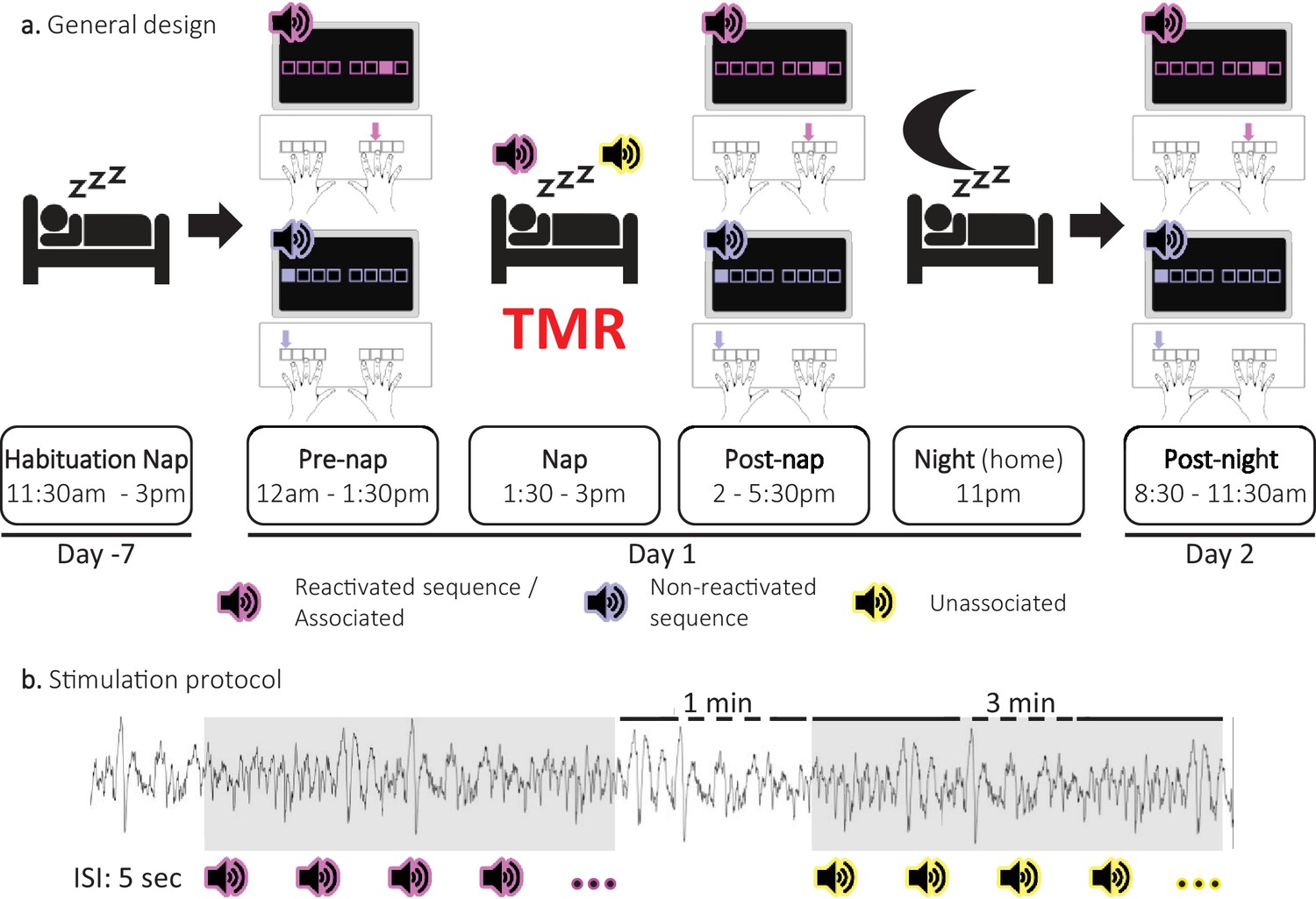
Experimental protocol.

(a) General design. Following a habituation nap that was completed approximately one week prior to the experiment, participants underwent a pre-nap motor task session, a 90 minute nap episode monitored with polysomnography during which targeted memory reactivation (TMR) was applied and a post-nap retest session. Participants returned to the lab the following morning to complete an overnight retest (post-night). During the motor task, two movement sequences were learned simultaneously and were cued by two different auditory tones. For each movement sequence, the respective auditory tone was presented prior to each sequence execution (i.e. one tone per sequence). One of these specific sounds was replayed during the subsequent sleep episode (Reactivated) and the other one was not (Non-reactivated). During the NREM 2–3 stages of the post-learning nap, two different sounds were presented. One was the sound associated (Associated) to one of the previously learned sequences, that is to the reactivated sequence, and one was novel, that is not associated to any learned material (Unassociated). (b) Stimulation protocol. Stimuli were presented during three-minute stimulation intervals of each cue type alternating with a silent 1 minute period (rest intervals). The inter-stimulus interval (ISI) was of 5 sec. The stimulation was manually stopped when the experimenter detected REM sleep, NREM1 or wakefulness.

Results

The analyses presented in the current paper that were not pre-registered are referred to as exploratory.

Behavioral data

As per our pre-registration, behavioral analyses focused on performance speed (i.e. response time (RT) on correct key presses) on the motor sequence learning task measured at three time points: pre-nap, post-nap, and post-night (Figure 1a). Results of the analyses on performance accuracy are presented in Figure 2—figure supplement 1.

Analyses of the pre-nap training data indicated that participants learned the two sequence conditions (reactivated and non-reactivated sequences) to a similar extent during initial learning (16 blocks of training; main effect of Block: F(15, 345)=34.82; p-value = 2.04e-26; η²=0.6; main effect of Condition: F(1, 23)=0.16; p-value = 0.69; Block by Condition interaction: F(15, 345)=1.09; p-value = 0.37; Figure 2a). After initial training, participants were offered a short break (~5 min) and were then tested again on the learned motor sequences. This short pre-nap test session was designed to offer a fatigue-free measure of the end-of-training, asymptotic performance to be used as baseline for the computation of subsequent offline changes in performance (see description below) (Pan and Rickard, 2015). Before computing offline changes in performance, we first assessed whether participants reached stable and similar performance levels between conditions during the pre-nap test session. Results showed that while performance reached similar levels between conditions (4 blocks; main effect of Condition: F(1,23) = 3.39e-5; p-value = 0.99; Block by Condition interaction: F(3,69) = 1.21; p-value = 0.31), asymptotic performance levels were not reached as shown by a significant Block effect (F(3,69) = 6.67; p-value = 0.001; η²=0.22). To meet the performance plateau pre-requisite to compute offline changes in performance, the first block of the pre-nap test session driving this effect was removed from further analyses. Performance on remaining blocks was stable as indicated by a non-significant Block effect (F(2,46) = 1.56; p-value = 0.22). Similar to above, the main effect of Condition (F(1,23) = 0.04; p-value = 0.85) and the Block by Condition interaction (F(2,46) = 1.81; p-value = 0.18) were not significant. Altogether, these results indicate that a performance plateau was ultimately reached and both sequence conditions were learned similarly (Figure 2a).

Figure 2 with 2 supplements see all
Behavioral results.

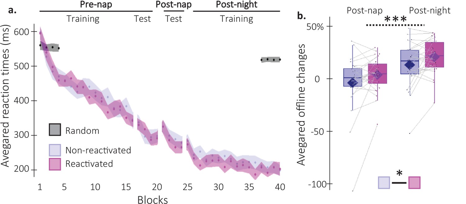
(a) Performance speed (N = 24; mean reaction time in ms) across participants plotted as a function of blocks of practice during the pre- and post-nap sessions (+/-standard error in shaded regions) for the reactivated (magenta) and the non-reactivated (blue) sequences and for the random SRTT (Black overlay). (b) Offline changes in performance speed (N = 24; % of change) averaged across participants (box: median (horizontal bar), mean (diamond) and first(third) as lower(upper) limits; whiskers: 1.5 x InterQuartile Range (IQR)) for post-nap and post-night time-points and for reactivated (magenta) and non-reactivated (blue) sequences. Using a repeated-measure ANOVA, the results highlighted a main effect of Time-point (***: p-value <0.001) and a main effect of Condition (*: p-value <0.05). Note that the main effect of condition is marginally significant when excluding the extreme participant (p=0.077).

Post-nap and post-night offline changes in performance were then computed for both conditions as the relative change in speed between the three plateau blocks of the pre-nap test and the first four blocks of the post-nap and post-night sessions, respectively. As such, improvement in performance from training to retest (i.e. faster performance at retest compared to training) was reflected by positive offline changes in performance. A repeated measures analysis of variance (rmANOVA) performed on offline changes in performance with Time-point (post-nap vs. post-night) and Condition (reactivated vs. non-reactivated) as within-subject factors showed a significant Time-point effect, whereby changes in performance were significantly higher at the post-night as compared to the post-nap retest (F(1,23) = 46.53; p-value = 5.89e-7; η²=0.67; Figure 2b). Critically, offline changes in performance for the reactivated sequence were significantly higher than for the non-reactivated sequence (Condition effect: F(1,23) = 4.75; p-value = 0.0397; η²=0.17). The Condition by Time-point interaction was not significant (F(1,23) = 7.42e-4; p-value = 0.98). In conclusion, our behavioral results indicate a TMR-induced enhancement in performance that did not differ across nap and night intervals.

Electrophysiological data

Participants’ sleep was recorded using a 6-channel EEG montage during a 90-min episode following learning. Sleep was monitored online and sounds were presented during NREM sleep stages. Sleep characteristics resulting from the offline sleep scoring as well as the distribution of auditory cues across sleep stages are shown in in Supplementary file 1. Briefly, results indicate that all the participants slept during the nap (average total sleep time: 67 min; average sleep efficiency: 74.9%) and that cues were accurately presented in NREM sleep (average stimulation accuracy: 88.4%).

Event-related analyses

Event-related analyses assessed the effect of the sound condition (i.e. associated vs. unassociated) on both the potentials (ERP) but also the oscillatory activity (time-frequency analyses) evoked by the auditory cues.

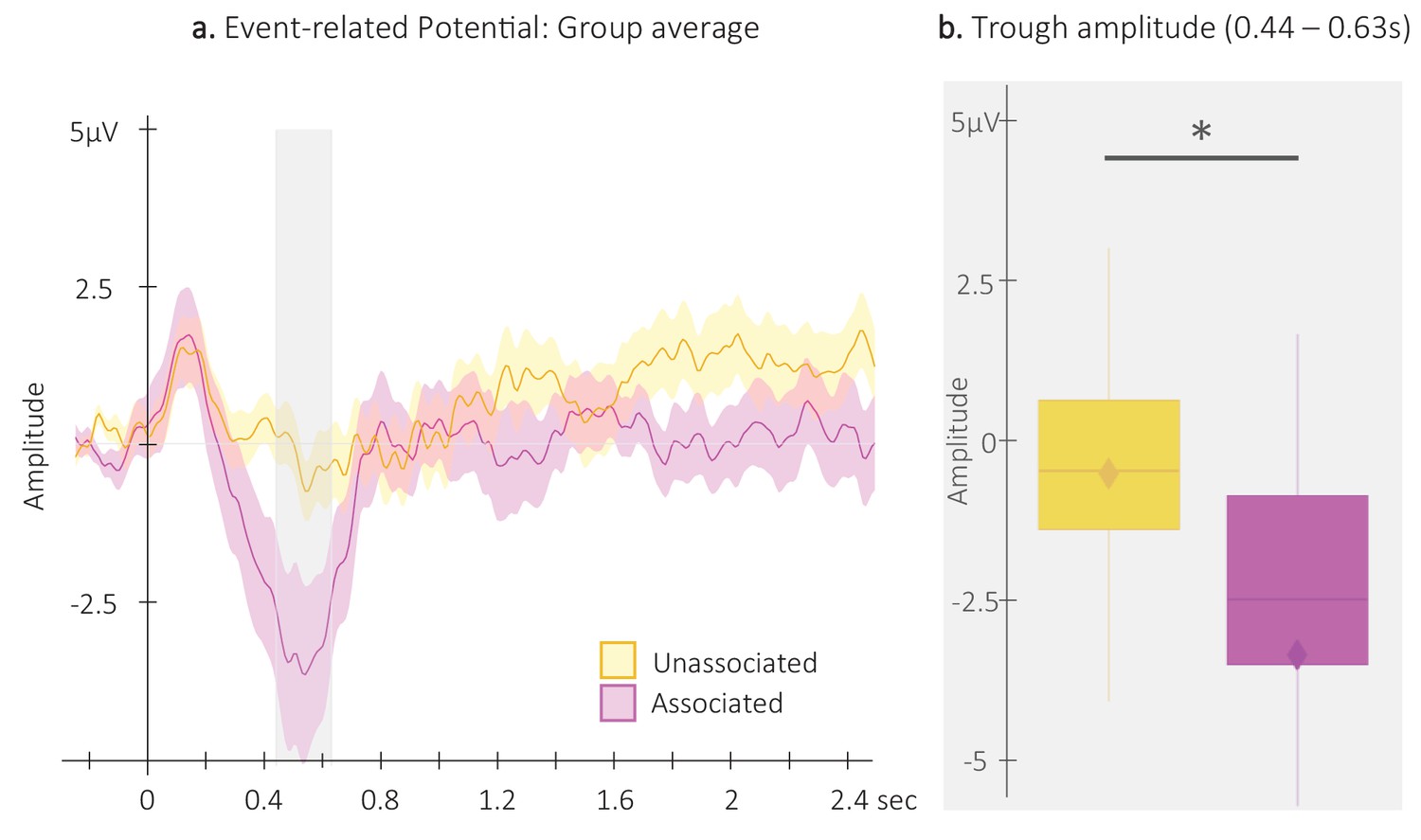
For the analyses of the auditory evoked potentials, we first computed ERPs on each EEG channel (see Figure 3—figure supplement 1 for channel level data) separately for associated and unassociated auditory cues presented during NREM2-3 stages and subsequently averaged ERPs across channels (Figure 3a). ERP amplitude was extracted for the 2 conditions from the temporal window highlighted in Figure 3a in which the amplitude of the auditory responses across conditions was significantly lower (trough) than zero (from 0.44 to 0.63 s relative to cue onset, see Figure 3—figure supplement 2 and Figure 3—figure supplement 3 for across- and within-channel level data, respectively). Between-condition comparisons using Wilcoxon signed-rank test showed that the amplitude of the ERP trough was significantly deeper (V=75, p-value = 0.016) following associated as compared to unassociated cues (Figure 3b).

Figure 3 with 3 supplements see all
Event-related potentials (ERP).

(a) Potentials averaged across all EEG channels and all participants (N = 24; +/-standard error in shaded regions) evoked by the associated (magenta) and the unassociated (yellow) auditory cues from –0.3 to 2.5 s relative cue onset. The gray region represents the temporal window (trough) in which ERPs across conditions were significantly different from zero. (b) ERP amplitude (N = 24; box: median (horizontal bar), mean (diamond) and first(third) as lower(upper) limits; whiskers: 1.5 x IQR) extracted from the temporal window highlighted in panel a, that is at 0.44 – 0.63 s post-cue onset (trough) in each condition. *: p-value <0.05 (Wilcoxon signed-rank test).

For the analyses of the auditory evoked oscillatory activity, we investigated whether EEG sigma oscillation power (12–16 Hz) evoked by the auditory cues on each channel was modulated by the different stimulation conditions in the 2.5 s following the cue onset. Note that, for completeness, time-frequency analyses were performed on a wider frequency range (5–30 Hz) and that analyses outside the sigma band were considered as exploratory. Cluster Based Permutations (Maris and Oostenveld, 2007) (CBP) tests computed on power averaged across all channels did not highlight any significant clusters between the two auditory cues.

Sleep event detection

Slow waves (SWs) and spindles were detected automatically (Vallat, 2020) on all EEG channels in all NREM2-3 sleep epochs (thus including associated and unassociated sound stimulation intervals as well as non-stimulation intervals, see Figure 1b). The detection tool identified on average 424.8 [95% CI 328–521.6] slow waves and 98 [95% CI: 82.8–113.2] spindles averaged across channels during the nap episode (see methods for details on the detection algorithms and in Supplementary file 2 for the number of events detected on each channel and each condition).

Concerning the detected SWs (Figure 4a), both peak-to-peak (PTP) amplitude and density (averaged across all EEG channels) were greater for the associated as compared to the unassociated stimulation intervals (amplitude: t=2.7; df = 21; p-value = 0.009; Cohen’s d=0.55; and density V=197; p-value = 0.01; r=0.58). Exploratory analyses including the detected SWs in the non-stimulation (rest) intervals did not highlight PTP amplitude differences between the rest intervals and the two types of stimulation intervals (rest vs. associated: t=0.82; df = 21; p-value = 0.42; rest vs. unassociated: t=–0.92; df = 21; p-value = 0.42; Figure 4b–c). However, SW density was significantly lower during the rest as compared to the stimulation intervals, regardless of the cue type (rest vs. associated: V=232; p-uncorrected=0.0002; p-FDR=0.0004; r=0.66; rest vs. unassociated: V=224; p- uncorrected = 0.0008; p-FDR=0.00081; r=0.6; Figure 4d). Altogether, these results indicate that auditory stimulation induced an overall increase in SW density, and, more importantly, that the associated sounds resulted in an increase in SW amplitude and density as compared to the unassociated sounds.

Detected Slow Waves (SWs).

(a) Average at the negative peak (N = 22; +/-standard error) across all detected slow waves on all channels during the associated (magenta) and unassociated (yellow) stimulation intervals as well as in the rest (i.e. unstimulated) intervals (gray). (b) Zoom on the negative peak of the detected SWs. Shaded regions represent SEM. (c) Peak-to-peak SW amplitude (μV) was higher for associated as compared to unassociated sounds (Student t-test). (d) SW density (number of SWs per total time in minutes spent in stimulation or rest intervals) was higher during stimulation as compared to rest intervals and for associated as compared to unassociated sounds (Wilcoxon signed-rank test). Box: median (horizontal bar), mean (diamond) and first(third) as lower(upper) limits; whiskers: 1.5 x IQR; *: p-value <0.05; **: p-value <0.01; ***: p-value <0.001; n.s.: not significant .

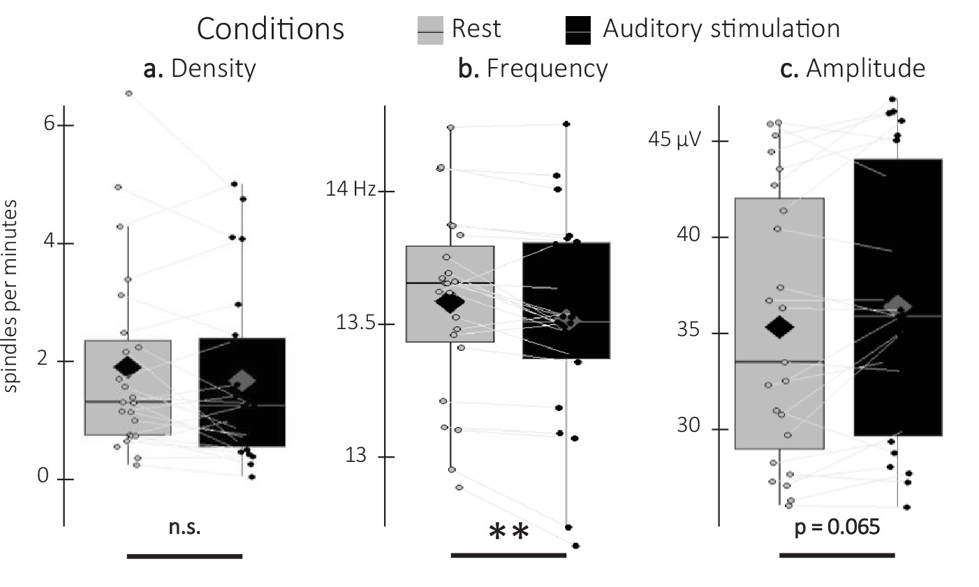
Sleep spindle density averaged across all channels did not differ between associated and unassociated stimulation intervals (V=98, p-value = 0.89). Similarly, exploratory analyses on additional spindle features including amplitude and frequency did not yield any significant differences between stimulation conditions (all p-values > 0.2). As no effect of stimulation was observed on spindle characteristics, the two conditions were pooled together in exploratory analyses including spindles detected during rest intervals (Figure 5). Results show that spindle density did not differ between stimulation and rest intervals (V=97, p-value = 0.22). Interestingly, the difference in spindle amplitude was marginally significant with higher amplitudes during the auditory stimulation intervals as compared to the rest intervals (V=199; p-value = 0.065; r=0.73), whereas spindle frequency showed the opposite pattern (t=–3.42; df = 22; p-value = 0.005; Cohen’s d=0.71). In summary, these results indicate that while auditory stimulation altered spindle features (frequency and amplitude to a lesser extent) as compared to rest, the two sound conditions did not differently influence these characteristics.

Detected spindles.

(a) Spindle density (number of spindles per total time in minute spent in stimulation or rest intervals) did not differ between stimulation intervals (irrespective of sound type; black) and rest (gray) intervals (Wilcoxon signed-rank test). (b) Spindle frequency (Hz) was lower during stimulation as compared to rest intervals (Student t-test). (c) Spindle amplitude (µV) was higher during stimulation as compared to rest intervals. All spindle features were averaged across channels (Wilcoxon signed-rank test). N = 23; Box: median (horizontal bar), mean (diamond) and first(third) as lower(upper) limits; whiskers: 1.5 x IQR; **: p-value <0.01; n.s.: not significant.

Phase-amplitude coupling

We investigated whether the phase of the slow oscillations in the 0.5–2 Hz frequency band was coupled to the amplitude of sigma (12–16 Hz) oscillations following either the auditory cue or the negative peak of the detected (i.e. spontaneous) SWs. The analyses presented below focus on the comparison between conditions but see Figure 6—figure supplement 1 for coupling analyses performed within each stimulation condition and at rest.

Event-related phase-amplitude coupling (ERPAC) analyses were performed across channels on a wider frequency range (7–30 Hz) for completeness; thus, analyses outside the pre-registered sigma band (see red frame in Figure 6) are considered exploratory. The ERPAC values locked to the auditory cues were compared between the two stimulation conditions. The CBP test did not highlight any significant clusters (alpha threshold = 0.025, cluster p-value = 0.44). The preferred coupling phase, which represents the phase at which the maximum amplitude is observed, did not significantly differ between conditions (F(1,46) = 0.3, p-value = 0.9). These results suggest that the stimulation conditions did not influence the coupling between the phase of the slow oscillations and the amplitude of sigma oscillations at the auditory cue.

Figure 6 with 3 supplements see all
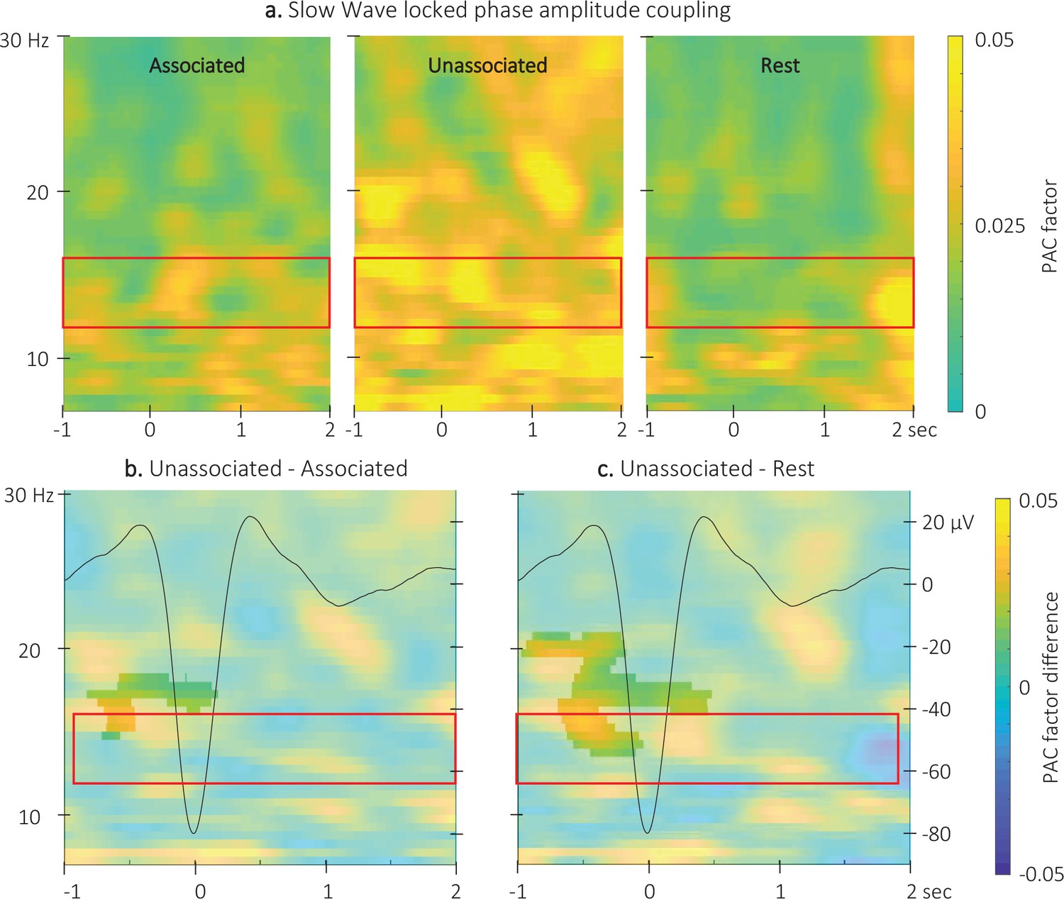
Event related phase-amplitude coupling locked to the detected slow wave negative peaks.

(a) Time-Frequency Representation (TFR) of group average (N = 22) coupling strength between the phase of the 0.5–2 Hz frequency band and the amplitude from 7 to 30 Hz (y-axis) from –1 to 2 s (x-axis) relative to SW negative peak for the three interval types. (b) ERPAC was significantly higher during the unassociated as compared to the associated sound intervals in the highlighted cluster (cluster-based permutation test). (c) ERPAC was significantly higher during the unassociated sound as compared to the rest intervals in the highlighted cluster (cluster-based permutation test). Red frames indicate the pre-registered sigma frequency band of interest. Superimposed on the TFR in panels b and c (black line): SW grand average across individuals and conditions (N = 22; y-axis on right).

Comparison of the ERPAC locked to the negative peak of the SWs (Figure 6 and Figure 6—figure supplement 2 for channel level data) between stimulation conditions revealed a significant cluster (alpha threshold = 0.025, cluster p-value = 0.024; Cohen’s d=–0.56). Specifically, the coupling between the phase of the signal in the 0.5–2 Hz frequency band and the amplitude of the signal in the 14–18 Hz frequency band was significantly stronger around the negative SW peak (from –0.8 to 0.2 s relative to negative peak) during unassociated as compared to associated stimulation intervals (Figure 6b). The exploratory comparison between rest and associated stimulation intervals did not reveal any significant clusters (alpha threshold = 0.025, all cluster p-values > 0.6) but a significant cluster was observed between unassociated stimulation and rest (alpha threshold = 0.025, cluster p-value = 0.001; Cohen’s d=0.53; Figure 6c). This cluster was observed between 13.5 and 20 Hz and –1–0.5 s around the negative peak of the SW. The preferred phases in each of the conditions were not significantly different (associated vs. unassociated: F(1,42) = 0;007, p-value = 0.94; associated vs. rest: F(1,42) = 0.01, p-value = 0.91; unassociated vs. rest: F(1,42) = 0.3, p-value = 0.87; see Figure 6—figure supplement 1). Altogether, these results suggest that slowand sigma oscillation coupling observed just before the onset of the SW was stronger during unassociated as compared to associated and rest intervals but that the preferred coupling phase was not modulated by the experimental conditions.

Correlational analyses

Correlation analyses between the TMR index (i.e. the difference in offline changes in performance – averaged across time points – between the reactivated and the non-reactivated sequence) and the density of SW and spindles as well as with the amplitude of the ERP did not yield any significant results (density of spontaneous SW: S=2486, p-value = 0.97) density of spontaneous spindles S=1412, p-value = 0.24; amplitude of the negative peak of the ERP S=2282, p-value = 0.73. However, the correlational CBP analysis between the TMR index and the difference in TF power elicited by the different auditory cues highlighted one significant cluster (alpha threshold = 0.025, cluster centered on 0.5 s post-cue p-value = 0.022, rho = - 0.46; Figure 7a and Figure 7—figure supplement 1 for channel level data). For illustration purposes, we extracted the difference in TF power within the significant cluster included in the pre-registered frequency band (12–16 Hz) and from 0.35 to 1 s post-cue onset (see Figure 3). The resulting scatter plot presented in Figure 7b indicates that higher TMR index (i.e. greater behavioral benefit of TMR) was related to higher sigma oscillation power for the unassociated compared to the associated sound condition.

Figure 7 with 1 supplement see all
Correlation between power difference and TMR Index.

(a) Time-Frequency Representation (TFR) of the rho values issued from the correlation between the TMR index and the difference between the power elicited by the associated auditory cues and the unassociated ones (N = 24). Highlighted, the negative clusters in which the TMR index is significantly correlated with the difference in power (cluster-based permutation test). Red frame indicates the pre-registered sigma frequency band of interest. Superimposed on the TFR (black line): Grand average across individuals (N = 24) and conditions of event related potentials elicited by the auditory cues (y-axis on right). (b) Negative correlation between the difference in power elicited by the associated and unassociated cues (0.35–1 s post-cue, 12–16 Hz) and the TMR index (dots represent individual datapoints).

Finally, with respect to ERPAC-TMR index correlation analyses, no significant correlation was observed between the auditory-locked ERPAC metrics and the TMR index (alpha threshold = 0.025, cluster p-values >0.09). In contrast, cluster-based permutation correlational tests performed between the 12 and 16 Hz TFR SW-locked ERPAC difference between the two conditions and the TMR index revealed a significant cluster. Results show that the associated vs. unassociated difference in coupling strength between the phase of the signal in the 0.5–2 Hz frequency band and the amplitude of the signal in the 14.5–17 Hz frequency band, just after the SW peak (0.5 and 1 s), was positively correlated with the TMR index (alpha threshold = 0.025, cluster p-value = 0.0499, rho = 0.55; Figure 8a and Figure 8—figure supplement 1 for channel level data). For illustration purposes, we extracted the difference in ERPAC in the significant cluster included in the pre-registered frequency band (between 14.5 and 16 Hz) from 0.55 to 1.05 s. The resulting scatter plot (Figure 8b) indicates that the stronger the phase-amplitude coupling during associated as compared to the unassociated stimulation intervals, the higher the TMR index.

Figure 8 with 1 supplement see all
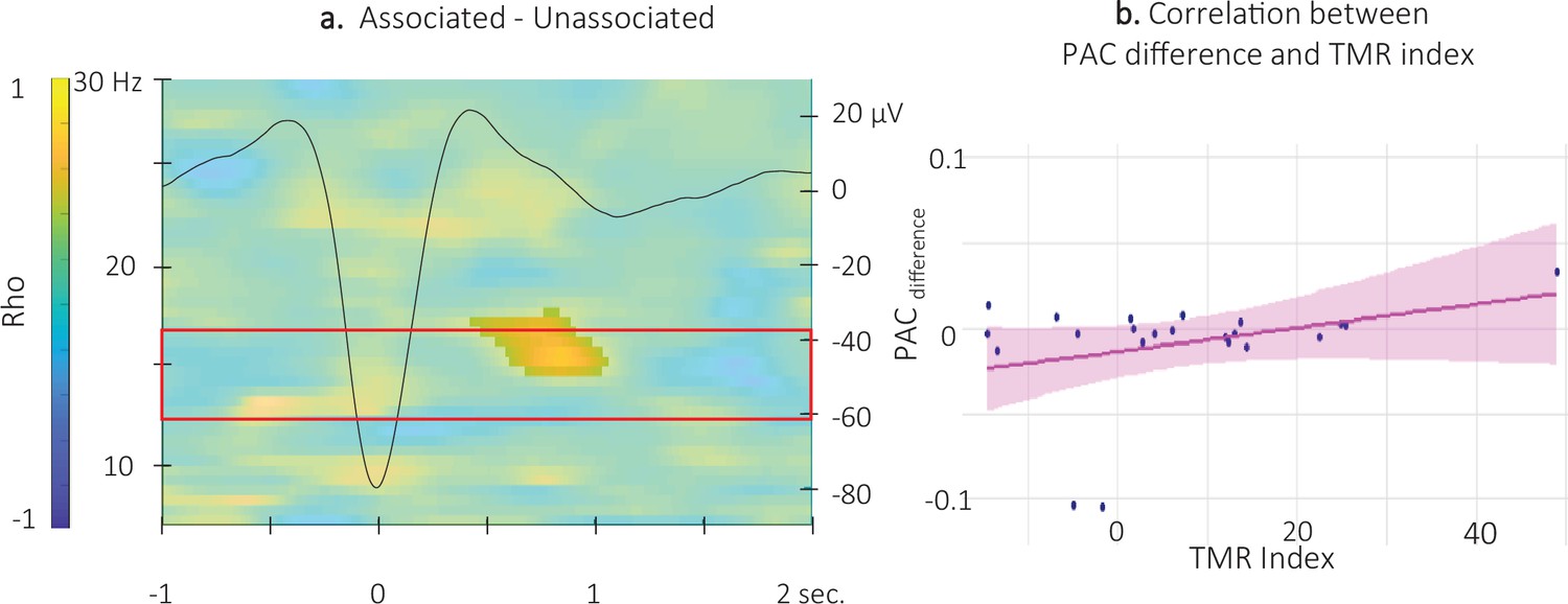
Correlation between SW-locked event related phase-amplitude coupling difference and TMR Index.

(a) Time-Frequency Representation (TFR) of the rho values issued from the correlation between the TMR index and the difference between the SW-locked ERPAC during the associated vs. unassociated stimulation intervals (N = 22). Highlighted, the positive cluster in which the TMR index is significantly correlated with the difference in SW-locked ERPAC (cluster-based permutation test). Superimposed on the TFR (black line): SW grand average across individuals and conditions. Red frame highlights the pre-registered sigma frequency band of interest. (b) Positive correlation between the SW-locked ERPAC difference (0.55–1.05 s post negative peak, 14.5–17 Hz) and the TMR index (dots represent individual datapoints).

Discussion

In the present study, we examined the impact of auditory TMR on motor memory consolidation as well as the neurophysiological processes supporting reactivation during sleep. Our results demonstrate a TMR-induced behavioral advantage such that offline changes in performance were larger on the reactivated as compared to the non-reactivated sequence. These behavioral results are in line with earlier motor learning studies showing improvement in performance after auditory (Schönauer et al., 2014; Antony et al., 2012; Cousins et al., 2016) or olfactory (Laventure et al., 2016) TMR during sleep. As opposed to earlier TMR research though, the current results suggest that TMR-induced consolidation is not a protracted process that needs additional time and/or sleep to develop (Cairney et al., 2018), as a behavioral advantage could already be observed immediately after the TMR episode. Also, in contrast to earlier work showing that TMR effects can be transient (Cousins et al., 2016), the current data indicate that the effect of TMR on motor performance was sustained overnight. It remains unclear whether these discrepancies are related to the nature of the task (e.g. declarative vs. motor), the sensory stimulus used for reactivation (words vs. sound) or the duration of the reactivation / sleeping episode (nap vs. night). Nevertheless, our findings suggest that the TMR episode during a nap immediately following learning set the reactivated memory trace on a distinct yet parallel trajectory as compared to the non-reactivated memory trace.

TMR effects were also observed at the brain level such that electrophysiological responses differed according to whether they were evoked by associated or unassociated cues. Specifically, the amplitude of the negative component of the auditory ERP was higher for the sounds associated to the motor memory task as compared to the unassociated sounds. These results are in line with findings from earlier associative learning studies performed during wakefulness showing that auditory cues evoke larger responses after conditioning (i.e. after they are associated to another stimulus) and that ERP amplitude is restored to pre-association levels after extinction (see Christoffersen and Schachtman, 2016 for a review). The current findings also extend prior observation of a modulation of auditory-TMR-evoked responses during sleep (Rudoy et al., 2009). This earlier study showed that auditory cues presented during post-learning sleep evoked larger ERPs when they were associated to items better remembered at subsequent recall as compared to cues associated to less remembered items. Our findings not only concur with this post-hoc analysis, but also provide the first direct evidence of an ERP modulation based on the memory content of the cue during post-learning sleep. This difference in brain potentials during sleep might be seen as the neural signature of the plasticity processes that occurred during learning. Not exclusive to the previous speculation, such effects might also be attributed to the (re)processing of the memory trace during post-learning sleep. Importantly, one could argue that the difference in ERP amplitude observed in the present study might be due to familiarity effects, as the unassociated sound might have been perceived as novel as compared to the associated sound. We argue that this is unlikely as new or rare auditory stimuli usually present larger negative amplitudes as compared to old or frequent sounds during both sleep and wakefulness (e.g. FN 400 [Rugg and Curran, 2007; Paller et al., 2012]) for old/new paradigms during wake and mismatch negativity components for oddball paradigms during both wake and sleep (Näätänen et al., 2007; Ruby et al., 2008). Instead, we propose that the auditory evoked brain responses observed in the current study reflect the (re)processing of the motor memory trace that was encoded during initial learning. It is worth noting that the negative peak of the potential evoked by the unassociated cues was not only lower (i.e. less negative) than for the associated cues but was also sometimes even absent on some channels (see Figure 3—figure supplement 1). These observations are partly in line with earlier research (Cairney et al., 2018) but contradict other findings. For example, Weigenand et al., 2016 as well as Schreiner and Rasch, 2015 observed significant negative responses evoked by control sounds or by sounds that were associated to later forgotten items. These discrepancies remain unclear but might in part be explained by methodological differences that are known to influence the amplitude of ERPs (e.g. sleep cycle stimulated, electrode(s) examined, number of stimulation repetitions provided).

In addition to the modulation of auditory-evoked responses described above, the properties of the detected (spontaneous) SWs were influenced by sound presentation and sound condition. Specifically, SW density was higher during sound presentation as compared to rest and the density and amplitude of the SWs were greater during intervals of associated – as compared to unassociated – cue stimulation. The effect of sound presentation on SW characteristics is in line with previous work showing sound-related entrainment of SW trains and increase in SW amplitude during sleep (Ngo et al., 2013a; Ngo et al., 2013b; Ngo et al., 2015; Ngo et al., 2019). More importantly, in line with the ERP results, our data show that the memory content of the cue modulated SW physiology above and beyond the mere effect of sound presentation. This is the first evidence, to the best of our knowledge, of a modulation of SW physiology based on the relevance of the sensory cues presented during sleep. We speculate that the processing of the memory content associated to the cue resulted in enhanced SW activity. Specifically, the greater amplitude of the SWs during associated sound intervals might reflect neural synchronization (Carrier et al., 2011; Esser et al., 2007) known to promote sleep-dependent plasticity processes for example (Born and Wilhelm, 2012; Ngo et al., 2013b). We thus propose that the TMR-effect observed in this study might therefore be mediated by SWs likely in relation with spindle activity.

While the characteristics of spontaneous spindles (amplitude and frequency) were only modulated by sound presentation and not sound condition, the properties of sigma oscillations (i.e. its amplitude and its coupling with the SO phase) were differently affected by the cue type and related to the TMR-induced behavioral advantage. The observation of a modulation of spindle characteristics irrespective of the sound condition suggests that spindle activity (in term of events) during reactivation is not related to motor memory processing per se. This stands in contrast with earlier reports of spindle-mediated effect of TMR on the consolidation of both declarative (Cairney et al., 2018) and motor (Laventure et al., 2016; Cousins et al., 2016) memory tasks. It is worth noting, however, that this earlier work did not compare different stimulus conditions as in the present study. Nonetheless, this previous research demonstrated that reactivation was related to an increase in spindle features (amplitude and frequency) that were linked to the TMR-induced motor performance advantage (Laventure et al., 2016).

Importantly, it is worth explicitly stating that our results do not rule out the involvement of spindle activity in TMR-related motor memory consolidation processes. Recent evidence has brought forward the idea that spindle event detection in general is less sensitive than the study of the sigma rhythm as a whole (Dimitrov et al., 2021). In line with these observations, our results show that sigma oscillation properties – as opposed to spindle events – were modulated by the sound condition and that such modulation was related to the TMR-induced behavioral advantage. Specifically, higher coupling between sigma oscillation amplitude and the SO phase, for associated as compared to unassociated sounds, on the descending phase following the peak of the SW was correlated with the TMR index. To the best of our knowledge, this is the first time that the strength of the coupling between the SO phase and the amplitude of the sigma oscillations nested within the peak of the SW is directly related to a TMR-related behavioral advantage. Earlier studies comparing different age groups provided convincing, yet indirect, evidence that the precise temporal coordination of SO and sleep spindles represents a critical mechanism for sleep-dependent memory consolidation (Muehlroth et al., 2019; Helfrich et al., 2018). The timing reported in this earlier work is consistent with the current data showing increased SW-sigma coupling on the descending phase following the peak of the SW. Our results are also in line with previous frameworks proposing that sigma oscillation (Cairney et al., 2018) / spindles (Antony et al., 2019) offer a privileged time window for relevant memories to be reinstated during sleep. Together with evidence that TMR boosted SW features, the current data suggest that both SWs and sigma oscillations play a critical role in the reactivation of motor memories.

In addition to the modulation of neurophysiological responses described above and triggered by the associated sounds, we report an intriguing pattern of brain results for the unassociated sounds. Specifically, the coupling between sigma amplitude and the SO phase was strengthened for unassociated sounds just before the onset of the SW negative peak. Furthermore, we observed that the increase in sigma power nested in the trough of the auditory evoked potential for unassociated (as compared to associated) sounds was related to higher TMR-induced performance enhancement. It is tempting to speculate that sigma oscillations might prevent the processing of unassociated/irrelevant sounds during post-learning sleep which might in turn be reflected by a decrease in the amplitude of the slow electrophysiological responses (i.e. smaller ERP and SWs) during non-associated sound intervals. We argue that sigma oscillations might play the role of a gatekeeper for the consolidation process and protect the motor memory trace against potential interfering effects induced by the unassociated sounds which might in turn potentiate the effect of TMR at the behavioral level. In order to further examine this possibility, we performed additional exploratory analyses testing for potential relationships between the SW-sigma coupling observed during unassociated stimulation intervals and slow electrophysiological responses (see Figure 6—figure supplement 3). Results showed a negative correlation between SW-sigma coupling and SW features such that higher coupling was related to lower SW amplitude and density during unassociated stimulation intervals. These results provide further support for the protective effect of sigma oscillations (nested in the trough of slow oscillations) against potential interfering effects induced by the unassociated sounds. These assumptions are also in line with a growing body of literature pointing towards a sensory gating role of spindle activity / sigma oscillations (Dang-Vu et al., 2011; Schabus et al., 2012) that might be critical to facilitate the memory consolidation process during sleep (Schreiner and Staudigl, 2020; Antony et al., 2019). Specifically, it has been proposed that a function of the thalamus is to suppress distraction and gate information processing via alpha/beta oscillations during wakefulness (Jensen and Mazaheri, 2010) and sigma oscillations during sleep (Chen et al., 2015). Further support for the gating hypothesis comes from observations of both increased arousal threshold as well as decreased amplitude of auditory ERP when sounds are presented simultaneously to a spindle event (Yamadori, 1971; Cote et al., 2000). Along the same lines, previous studies using simultaneous EEG-fMRI recordings showed that the BOLD responses in relation to sound processing are inconsistent or even absent when sounds occur during sleep spindles or before the negative peak of the SW (Dang-Vu et al., 2011; Schabus et al., 2012). The present data therefore suggest that the precise SO-sigma coordination does not only play a role in the reinstatement of relevant memories, but is also critical to prevent the processing of irrelevant information during post-learning sleep. These observations are remarkably in line with recent theoretical views putting forward the concept that temporally precise SO-spindle coupling might not convey only memory-specific information (Helfrich et al., 2021). It is argued that while synchronized states might trigger memory reactivation, the underlying neural activity might offer limited opportunities for information processing. Our data concur with this theory as they suggest that SO-sigma coupling, depending on its temporal characteristics, either prevents the processing of irrelevant information or supports memory reactivation during post-learning sleep.

In conclusion, our results depict a complex organization of the different physiological processes supporting motor memory consolidation during post-learning sleep. While associated sounds appeared to boost SW features and SO-sigma coupling at the peak of the SW, unassociated sounds predominantly modulated the properties of the sigma oscillations at the trough of the slow oscillation. Our findings suggest a dual role of sigma oscillations whereby, depending on their temporal coordination with SWs, they either protect memories against irrelevant material processing or promote the reactivation of relevant motor memories; two processes that critically contribute to the motor memory consolidation process.

Materials and methods

This study was pre-registered in the Open Science Framework (https://osf.io/). Our pre-registration document outlined our hypotheses and intended analysis plan as well as the statistical models used to test our a priori hypotheses (available at https://osf.io/y48wq). Whenever an analysis presented in the current paper was not pre-registered, it is referred to as exploratory. Additionally, to increase transparency, any deviation from the pre-registration is marked with a (#) symbol and listed in Supplementary file 3 together with a justification for the change.

Participants

Young healthy volunteers were recruited by local advertisements to participate in the present study. Participants gave written informed consent before participating in this research protocol, approved by the local Ethics Committee (B322201525025) and conducted according to the declaration of World Medical Association, 2013. The participants received a monetary compensation for their time and effort. Inclusion criteria were: (1) left- or right-handed# (see point #1 of Supplementary file 3); (2) no previous extensive training with a musical instrument or as a professional typist, (3) free of medical, neurological, psychological, or psychiatric conditions, including depression and anxiety as assessed by the Beck’s Depression (Beck et al., 1996) and Anxiety (Beck et al., 1988) Inventories, (4) no indications of abnormal sleep, as assessed by the Pittsburgh Sleep Quality Index (Buysse et al., 1989); (5) not considered extreme morning or evening types, as quantified with the Horne & Ostberg chronotype questionnaire (Horne and Ostberg, 1976); and, (6) free of psychoactive or sleep-affecting medications. None of the participants were shift-workers or took trans-meridian trips in the 3 months prior to participation.

The sample size was determined with a power analysis performed through the G*Power software (Faul et al., 2007) and based on the paper of Cousins et al., 2016 which reports, to our knowledge, the closest paradigm to the present one in the motor memory domain (see details in the pre-registration). Sample size was estimated to 24 participants. Thirty-four participants took part in the study to reach this estimated sample size after participant exclusion. As per our pre-registration, participants were excluded if their sleep duration during the experimental nap was insufficient to provide at least 50 stimulations per condition (after EEG data cleansing). This cut-off aimed at providing enough events to reach sufficient signal-to-noise ratio for electrophysiological analyses. Ten participants did not reach this criterion; accordingly, 24 participants (12 females) completed the experimental protocol and were included in the analyses (see participants’ characteristics in Table 1).

Table 1
Participant characteristics and sleep characteristics leading up to the experimental session and vigilance assessments at time of testing.
N24 (12 females)
Age (yrs)21.9 ranging from 18 to 27
Edinburgh Handedness (Oldfield, 1971)78.6 [57.1–100]
Epworth Sleepiness Scale (Hoddes et al., 1972)7 [5.9–8.1]
Beck Depression Scale (Beck et al., 1996)1.5 [0.9–2.2]
Beck Anxiety Scale (Beck et al., 1988)1.8 [1.1–2.4]
PSQI (Buysse et al., 1989)3 [2.2–3.8]
Chronoscore (CRQ)(51)48.8 [45.6–51.9]
Sleep durationa
Mean across the 3 nights (minutes)
Night 1481.5 [461.5–501.5]
Night 2488.2 [471.2–505.2]
Night 3502 [482.1–521.8]
St. Mary’s questionnaire on Night 3 quality
Quality4.7 [4.3–5.1]
Duration (minutes)443.5 [423.3–463.8]
Psychomotor Vigilance Taskb
Pre-nap300.2ms [289.7–310.6]
Post-nap297.5ms [288.9–306]
Post-night294.7ms [285.1–304.2]
One-way rmANOVA resultsF(2,46)=1.47; P-value = 0.24
Stanford sleepiness score
Pre-nap Session2.4 [2.1–2.7]
Post-nap Session2.7 [2.3–3.1]
Post-night Session2.3 [1.9–2.7]
One-way rmANOVA resultsF(2,46)=1.69; P-value = 0.2
  1. Notes. Values are means [lower and upper limit of the 95% Confidence Interval - CI]. PSQI = Pittsburgh Sleep Quality Index; CRQ = Circadian Rhythm Questionnaire. REM: Rapid Eye Movement. a Sleep duration was computed as the mean across the actigraphy data and the sleep diary for the three nights before the experimental day. b Median of reaction times computed across the 100 trials of each session.

General design

Request a detailed protocol

This study employed a within-participant design (Figure 1). Participants were first invited, in the early afternoon, for a habituation nap during which they completed a 90-min nap monitored with polysomnography (PSG, see below for details). Approximately 1 week later, participants returned to complete the experimental protocol. Each participant followed a constant sleep/wake schedule (according to their own rhythm +/-1 hr) for the 3 days before the experiment. Compliance was assessed with sleep diaries and wrist actigraphy (ActiGraph wGT3X-BT, Pensacola, FL). Sleep quality and quantity for the night preceding the experimental visit was assessed with the St. Mary’s sleep questionnaire (Ellis et al., 1981; see Table 1 for results about sleep data before the experimental session). During the first experimental day, participants were trained on two motor sequences simultaneously (pre-nap session: between 12 pm-1:30 pm). During learning, each of these two sequences was associated to a particular sound. Only one of these two sounds was presented during the subsequent nap episode, corresponding to the associated sound linked to the reactivated sequence. At the behavioral level, the control condition consisted of the non-reactivated sequence (i.e. a sequence that was associated to a sound during learning but the sound was not presented during the subsequent nap interval). For electrophysiological analyses, a new, unassociated, sound (i.e. a sound to which participants were not exposed during the learning episode) was presented during the post-learning sleep, serving as a control condition. The nap occurred between 1:30 pm and 3 pm and was monitored with PSG. Sleep data were monitored online by an experimenter in order to send auditory stimulations during NREM2-3 stages. Performance on the reactivated and non-reactivated sequences was tested 30 min after the end of the nap to allow sleep inertia to dissipate (post-nap session: 2 pm-5:30 pm) and on day 2 after a night of sleep (not monitored with PSG) spent at home (post-night session: 8:30 am-11:30 am). At the beginning of each behavioral session, vigilance was measured objectively and subjectively using the Psychomotor Vigilance Task (Dinges and Powell, 1985) and Stanford Sleepiness Scale (Hoddes et al., 1972), respectively (see Table 1). Finally, general motor execution was tested at the beginning of the pre-nap session and at the end of the post-night session.

This design allowed to assess the specific impact of TMR on consolidation at the behavioral level, with the comparison between the changes in performance of the reactivated and non-reactivated sequences assessed during the post-nap and post-night sessions; and at the electrophysiological level, with the comparison between the neurophysiological responses to the reactivated associated sound vs. the unassociated sound that did not carry mnemonic information.

Stimuli and tasks

All tasks were performed on a laptop computer (Dell Latitude 5,490 run under Microsoft Windows 10 Enterprise) and were implemented in Matlab (Math Works Inc, Natick, MA, USA) Psychophysics Toolbox version 3 (Kleiner, 2007). Participants sat comfortably in front of the computer screen with the keyboard on their knees. This configuration allowed the participants to focus their gaze on the screen and not to look at their hands/movements. Distance between participants and the screen was approximately 70 cm but was self-selected by the participants based on comfort. The sound presentation was conducted using ER3C air tube insert earphones (Etymotic Research).

Acoustic stimulation

Request a detailed protocol

Three different 100 ms sounds were randomly assigned to the three conditions (reactivated/associated, not-reactivated, and unassociated), for each participant. The three synthesized sounds consisted of a tonal harmonic complex created by summing a sinusoidal wave with a fundamental frequency of 543 Hz and 11 harmonics with linearly decreasing amplitude (i.e. the amplitude of successive harmonics is multiplied by values spaced evenly between 1 and 0.1); white noise band-passed between 100 and 1000 Hz and a tonal harmonic complex created with a fundamental frequency of 1480 Hz and 11 harmonics with linearly increasing amplitude (i.e. the amplitude of successive harmonics is multiplied by values spaced evenly between 0.1 and 1). A 10 ms linear ramp was applied to the onset and offset of the sound files so as to avoid earphone clicks. At the start of the experiment, auditory detection thresholds were determined by the participants themselves using a transformed 1-down 1-up procedure (Levitt, 1971; Leek, 2001) separately for each of the three sounds. Subsequently, the sound pressure level was set to 1000% of the individual auditory threshold during the tasks and 140% for auditory stimulation during sleep, thus limiting the risk of awakening during the nap (Sterpenich et al., 2014). Before the start of the nap episode, participants were instructed that they may or may not receive auditory stimulations during the nap.

Motor task

Request a detailed protocol

A bimanual serial reaction time task (Nissen and Bullemer, 1987) (SRTT) was used to probe motor learning and memory consolidation processes. During this task, eight squares were horizontally presented on the screen meridian, each corresponding to one of the eight keys on the specialized keyboard and to one of the 8 fingers (no thumbs). The color of the outline of the squares alternated between red and green, indicating rest and practice blocks, respectively. During the practice blocks, participants had to press as quickly as possible the key corresponding to the location of a green filled square that appeared on the screen. After a response, the next square changed to green with a response-to-stimulus interval of 0 ms. After 64 presses, the practice block automatically turned into a rest block and the outline of the squares changed from green to red. The rest interval was 15 s.

The order in which the squares were filled green (and thus the order of the key presses) either followed a sequential or pseudo-random pattern. In the sequential SRTT, that is assessing motor sequence learning, participants were trained simultaneously on two different eight-element sequences (sequence A: 1 6 3 5 4 8 2 7; sequence B: 7 2 6 4 5 1 8 3, in which 1 through 8 are the left pinky to the right pinky fingers respectively). Participants were explicitly told that the stimuli (and thus the finger presses) would follow two different repeating patterns composed of eight elements each, but were not told any further information. During each practice block, four repetitions of a specific sequence (e.g. sequence A) were performed, each separated by a 1 sec-interval. Then, after a 2 sec-interval, the four repetitions of the other sequence started (e.g. sequence B). The order of the two sequences was randomized within each block of practice. Each motor sequence was associated to a different tone that consisted of a single 100 ms auditory cue (see above). The auditory cue was presented before the beginning of each sequence repetition, that is before the first key press of the sequence that was to be performed. Accordingly, one single tone was associated to an eight-element sequence of finger movements. Participants were instructed to learn the sequence-sound association during task practice. The associations between sound-sequence (sounds 1, 2 and 3; sequence A, sequence B, and control sound presented during nap) and sequence-condition (sequences A and B; conditions reactivated and not-reactivated) were randomized, thus creating 12 different possible combinations of randomized variables. Each participant was pseudo-randomly assigned to one of these combinations, such that there were two participants per combination. For the random SRTT, the order of the eight keys was shuffled for each eight-element repetition and thus the number of each key press was constant across all random and sequential blocks. For both variants of the task, the participants were instructed to focus on both speed and accuracy.

For the pre-nap session, participants first completed 4 blocks of the random SRTT to assess general motor execution. Participants subsequently completed the sequential SRTT, which consisted of 16 blocks of training followed by 4 blocks of post-training test taking place after a 5 min break. This allowed the assessment of end of training performance after the further dissipation of physical and mental fatigue (Pan and Rickard, 2015). For the post-nap session, only 4 blocks of the sequential SRTT were completed to avoid extensive task practice before the final overnight retest. For the post-night session, 16 blocks of the sequential SRTT were performed, followed by 4 blocks of the random SRTT.

Between the training and test runs as well as after the post-night session, participants completed a generation task that aimed at testing explicit knowledge of the sequences as well as the strength of the association between the sequences and their corresponding auditory cues. During the generation task, participants were presented with the auditory cues specific to the learned sequences and were instructed to self-generate the corresponding motor sequences. Participants completed 4 consecutive attempts for each cue / sequence pair. The order of the pairs was randomized. Accuracy was emphasized during this task. A trial was classified as ‘correct’ if the key pressed by the participant was in the correct ordinal position with respect to the sequence acoustically cued. The percentage of correct ordinal positions was computed per sequence and per attempt. The generation accuracy per sequence was computed by averaging across attempts for each time point separately (pre-nap and post-night sessions). We tested whether generation accuracy of the reactivated sequence during the pre-nap generation task was correlated (Pearson’s correlation) to the TMR index. Results showed that there was no significant correlation between generation accuracy and the TMR index (r=0.25, t=1.22, df = 22, p-value = 0.24).

Polysomnography and targeted memory reactivation protocol

Request a detailed protocol

Both habituation and experimental naps were monitored with a digital sleep recorder (V-Amp, Brain Products, Gilching, Germany; bandwidth: DC to Nyquist frequency) and were digitized at a sampling rate of 1000 Hz (except for one participant (500 Hz) due to experimental error). Standard electroencephalographic (EEG) recordings were made from Fz, C3, Cz, C4, Pz, Oz, A1, and A2 according to the international 10–20 system (note that Fz, Pz and Oz were omitted during the habituation nap). A2 was used as the recording reference and A1 as a supplemental individual EEG channel. An electrode placed on the middle of the forehead was used as the recording ground. Bipolar vertical and horizontal eye movements (electrooculogram: EOG) were recorded from electrodes placed above and below the right eye and on the outer canthus of both eyes, respectively. Bipolar submental electromyogram (EMG) recordings were made from the chin. Electrical noise was filtered using a 50  Hz notch. Impedance was kept below 5 kΩ for all electrodes. During the experimental nap, PSG recordings were monitored by a researcher in order to detect NREM2-3 sleep based on the most recent sleep scoring guidelines from the American Academy of Sleep Medicine (Berry, 2018). To do so, PSG recordings were displayed online using 30-second-long epochs with EEG and EOG data filtered from 0.5 to 30 Hz and EMG data filtered between 20 and 200 Hz. When NREM2-3 sleep stages were reached, auditory cues were sent. The auditory stimulation was presented in a blocked design (Figure 1B). Namely, each type of auditory cue (associated or unassociated) was sent during 3-min-long stimulation intervals with an inter-stimulus interval of 5 s. The stimulation was stopped manually when the experimenter detected REM sleep, NREM1 or wakefulness. Intervals of stimulation for each sound were separated by a 1 min silent period (rest intervals).

Analysis

Statistical tests were performed with the open-source software (R Development Core Team, 2020; RStudio Team, 2020) and considered significant for p<0.05. When necessary, corrections for multiple comparisons was conducted with the False Discovery Rate (Benjamini and Hochberg, 1995) (FDR) procedure within each family of hypothesis tests (see details for each analysis below). Greenhouse-Geisser corrections was applied in the event of the violation of sphericity. Wilcoxon signed-rank tests were used when the Shapiro-Wilk test indicated non-normal distribution# (see point #6 of Supplementary file 3). F, t and V (or W) statistics and corrected p-values were therefore reported for ANOVAs, Student and Wilcoxon tests, respectively. Effect sizes are reported for significant comparisons using Cohen’s d for Student t-tests, r for Wilcoxon signed-rank test and η² for rmANOVAs using G*power (Faul et al., 2007). For correlation analyses, Spearman# test (see point #6 of Supplementary file 3) was used and S as well as corrected p-values were reported. Nonparametric CBP tests (Maris and Oostenveld, 2007) implemented in fieldtrip toolbox (Oostenveld et al., 2011) were used for high dimensional time and time-frequency data analyses (e.g. ERP, TF, and PAC analyses). CBP tests are composed of two subsequent tests. The first calculates paired t-tests (for contrast analyses) between conditions for each time points (or time-frequency points), which are then thresholded at a chosen p-value which sets the conservativeness of the test (reported as ‘cluster threshold’). Significant clusters are defined as showing a continuum of significant time (or time-frequency) points. Subsequently, the procedure is repeated 500 times on shuffled data in which the condition assignment within each individual is permuted randomly. On each permutation, the maximum t-value is retained, yielding a distribution of 500 t-values (for contrast analyses). Finally, this distribution is used as a reference to determine whether the statistical value (t in case of contrast analyses) of each cluster, as calculated on the real assignment of the conditions, is likely to come from the same probability distribution (p-value >0.05) or rather differs significantly from this random perturbation probability distribution (p-value <0.05). For CBP contrast analyses, Cohen’s d is reported while rho is reported for CBP correlations.

Behavior

Request a detailed protocol
Preprocessing
Request a detailed protocol

Motor performance on both the random and sequential SRTT was measured in terms of speed (correct response time (RT) in ms) and accuracy (% correct responses) for each block of practice. Note that RTs from individual correct trials were excluded from the analyses if they were greater than 3 standard deviations above or below the participant’s mean correct response time for that block (1.73% in total). Consistent with our pre-registration, our primary analyses were performed on speed.

The offline changes in performance on the sequential SRTT were computed as the relative change in speed between the pre-nap session (namely the 3 last blocks of practice#, see results and point #2 of Supplementary file 3 for details) and the post-nap session (4 blocks of practice) and the post-night session (4 first blocks of practice) separately for the reactivated and the non-reactivated sequences. A positive offline change in performance therefore reflects an increase of absolute performance from the pre-nap test to the post-nap or post-night tests. Additionally, we computed a TMR index, to be used in brain-behavior correlation analyses, which consisted of the difference in offline changes in performance - averaged across time points - between the reactivated and non-reactivated sequences. A positive TMR index reflects higher offline changes in performance for the reactivated as compared to the non-reactivated sequence.

Statistical analyses
Request a detailed protocol

We first assessed whether performance (speed and accuracy) significantly differs between conditions during initial training. To do so, two two-way rmANOVAs with Condition (reactivated vs. non-reactivated) and Block (1st rmANOVA on the 16 blocks of the pre-nap training and 2nd rmANOVA on the 4 blocks of the pre-nap test) as within-subject factors were performed on the sequential SSRT performance. Similar analyses testing for baseline differences between sequences A and B irrespective of the reactivation condition were performed. The results of these control analyses are presented in Figure 2—figure supplement 2. We then tested whether offline changes in performance on the sequential SRTT differed between reactivation conditions after a nap and night of sleep. This was done with a rmANOVA with Time-point (post-nap vs. post-night) and Condition (reactivated vs. non-reactivated) as within-subject factors on the offline changes in performance. Finally, to highlight that improvement in movement speed was specific to the learned sequences as opposed to general improvement of motor execution, we computed the overall performance change for both the sequential SRTT (first 4 blocks of pre-nap raining vs. 4 last blocks of post-night training collapsed across reactivated and non-reactivated sequences) and the pseudo-random version of the SRTT (4 blocks pre-nap session vs. 4 blocks post-night session). Two-tailed paired Student t-test revealed that overall performance changes in performance were significantly higher for the sequential SRTT as compared to the random SRTT (t=21.69, df = 23, p-value <2.2e-16; Cohen’s d=4.43). Thus, the RT decrease reported on the sequential SRTT in the result section reflect motor sequence learning rather than a mere improvement in motor execution.

Electroencephalography

Offline sleep scoring

Request a detailed protocol

A certified sleep technologist blind to the stimulation periods completed the sleep stage scoring offline according to criteria defined in Iber and Iber, 2007 using the software SleepWorks (version 9.1.0 Build 3042, Natus Medical Incorporated, Ontario, Canada). Data were visually scored in 30 s epochs and band pass filters were applied between 0.3 and 35 Hz for EEG signals, 0.3 and 30 Hz for EOG, and 10 and 100 Hz for EMG. A 50 Hz notch filter was also used (see Table 1 for details of extraction from scored data).

Preprocessing

Request a detailed protocol

EEG data preprocessing was carried out using functions supplied by the fieldtrip toolbox (Oostenveld et al., 2011). Specifically, data were cleaned by manually screening each 30-s epoch. Data segments contaminated with muscular activity or eye movements were excluded. Data were filtered between 0.1 and 30 Hz.

Event-related analyses

Request a detailed protocol

Event-related data analyses (i.e. auditory-evoked potentials and oscillatory activity) were performed with the fieldtrip toolbox (Oostenveld et al., 2011) with down sampled data (100 Hz). Auditory-evoked responses were obtained by segmenting the data into epochs time-locked to auditory cue onset (from –1 to 3 s relative to auditory cue onset after correction for onset-trigger lags) separately for the associated and unassociated auditory cues and averaged across all trials# (see point #3 of Supplementary file 3) in each condition separately. During cleaning, 1.03% [95% CI: 0.49–1.58] of the trials with stimuli sent during NREM2-3 stages were discarded. The remaining number of artifact-free trials was not significantly different between the two stimulation conditions (associated vs. unassociated, t=–0.5888, df = 23, p-value = 0.5617).

For event-related potentials (ERPs) analyses, individual ERPs computed on each channel were baseline corrected by subtracting mean amplitude from –0.3 to –0.1 s relative to cue onset. As our low-density EEG montage did not allow to perform fine topographical analyses, ERP data were averaged across all 6 EEG channels (but see Figure 3—figure supplement 1 and Figure 3—figure supplement 3 where channel level data are presented) data. In a first step, we used CBP approaches on ERP data computed across conditions to identify specific time windows during which significant brain activity was evoked by the auditory stimulation (i.e. where ERPs were significantly greater than zero). Results showed that across condition ERP was significantly different from zero between 0.44 and 0.63 sec at the trough (alpha threshold = 0.025, cluster p-value = 0.044; Cohen’s d=–0.56; see Figure 3—figure supplement 2). In a second step, ERP amplitude was then averaged within this specific time-window for the two conditions separately and compared using one-tailed paired Wilcoxon signed-rank test# (see point #6 of Supplementary file 3) with the hypothesis that ERP absolute amplitude at the trough is greater following the associated cues as compared to unassociated cues.

To analyze oscillatory activity, we computed Time-Frequency Representations (TFRs) of the power spectra per experimental condition and per channel. To this end, we used an adaptive sliding time window of five cycles length per frequency (Δt=5 /f; 20 ms step size), and estimated power using the Hanning taper/FFT approach between 5 and 30 Hz# (see point #4 of Supplementary file 3). Individual TFRs were converted into baseline relative change of power (baseline from –0.3 to –0.1 s relative to cue onset), thus highlighting power modulation following the auditory cues. All six EEG channels were then averaged (but see Figure 7—figure supplement 1 for channel level data). To identify significant evoked power modulation, TFR locked to auditory cues were compared between conditions using a CBP test between 5 and 30 Hz and from 0 to 2.5 sec relative to cue onset.

Sleep-event detection

Request a detailed protocol

Preprocessed cleaned data were down-sampled to 500 Hz and were transferred to the python environment. Slow waves and spindles were detected automatically in NREM2-3 sleep epochs on all the channels, by using algorithms implemented in the YASA open-source Python toolbox (Vallat, 2020; Vallat and Walker, 2021). Concerning the SW detection, the algorithm used is a custom adaptation of Massimini et al., 2004 and Carrier et al., 2011. Specifically, data were filtered between 0.3 and 2 Hz with a FIR filter using a 0.2 Hz transition resulting in a –6 dB points at 0.2 and 2.1 Hz. Then all the negative peaks with an amplitude between –40 and –200 μV and the positive peaks with an amplitude comprised between 10–150 μV are detected in the filtered signal. After sorting identified negative peaks with subsequent positive peaks, a set of logical thresholds are applied to identify the true slow waves: (1) duration of the negative peak between 0.3 and 1.5 sec; (2) duration of the positive peak between 0.1 and 1 sec; (3) amplitude of the negative peak between 40 and 300 µV; (4) amplitude of the positive peak between 10 and 200 µV and (5) PTP amplitude between 75 and 500 µV. Concerning spindle detection, the algorithm is inspired from the A7 algorithm described in Lacourse et al., 2019. Specifically, the relative power in the spindle frequency band (12–16 Hz) with respect to the total power in the broad-band frequency (1–30  Hz) is estimated based on Short-Time Fourier Transforms with 2-s windows and a 200ms overlap. Next, the algorithm uses a 300ms window with a step size of 100 ms to compute the moving root mean squared (RMS) of the filtered EEG data in the sigma band. A moving correlation between the broadband signal (1–30  Hz) and the EEG signal filtered in the spindle band is then computed. Sleep spindles are detected when the three following thresholds are reached simultaneously:(1) the relative power in the sigma band (with respect to total power) is above 0.2 (2) the moving RMS crosses the RMSmean +1.5 RMSSD threshold and (3) the moving correlation described is above 0.65. Additionally, detected spindles shorter than 0.5  s or longer than 2  s were discarded. Spindles occurring in different channels within 500ms of each other were assumed to reflect the same spindle. In these cases, the spindles are merged together.

SWs and spindles were detected in the stimulation intervals of both associated and unassociated sounds. One participant did not show any SW during the unassociated cue stimulation intervals and the minimal required number of SWs was not reached to perform the PAC in another participant. The two participants were thus excluded from the analyses on detected SWs. No spindles were detected during the associated cue stimulation intervals for another participant who was therefore excluded from the spindle analyses. With respect to the detected SWs, we extracted for each participant, each condition and channel, the mean PTP amplitude (µV) of SWs# (see point #3 of Supplementary file 3) as well as their density (number of SWs per total time in minutes spent in stimulation or rest intervals). These characteristics were then averaged across channels. Concerning the spindles, we extracted for each participant, condition and channel, spindle density (i.e. the number of spindles per total time in minutes spent in stimulation or rest intervals). Spindle amplitude (computed as the PTP amplitude (µV) in the sigma-filtered data) and frequency were also extracted for exploratory analyses. These different dependent variables were then averaged across channels and were compared using a one-tailed paired Student t-test (SW PTP and spindle Frequency) or Wilcoxon signed-rank (SW density, spindle density and amplitude) test# (see point #6 of Supplementary file 3) with the hypothesis that the associated, as compared to unassociated, stimulation intervals would exhibit higher values.

Furthermore, we performed exploratory analyses including the SWs and the spindles detected during rest intervals (i.e. NREM 2–3 epochs without auditory stimulation). In the case of SWs, we compared these values with those obtained for the associated stimulation intervals and the unassociated stimulation intervals using two two-tailed Student t-tests or Wilcoxon signed-rank tests (rest vs. associated stimulation intervals and rest vs. unassociated stimulation intervals). In the case of spindles, as spindle characteristics did not differ between stimulation conditions (see results), they were collapsed across stimulation conditions and compared to rest intervals using two-tailed Student t-tests or Wilcoxon signed-rank tests. Correction for multiple comparisons was performed using the FDR approach (Benjamini and Hochberg, 1995).

Phase-amplitude coupling

Request a detailed protocol

In order to perform coupling analyses, preprocessed cleaned data were first down-sampled to 500 Hz. Based on the low spatial resolution of our montage that did not allow fine topographical analyses and in order to increase the signal to noise ratio to enhance the quality of the phase estimation that is particularly sensitive to noise (Gross et al., 2013), we opted to average the data across channels (but see Figure 6—figure supplement 2 and Figure 8—figure supplement 1 for channel level data). Coupling analyses were then performed using the Event-Related Phase-Amplitude Coupling (ERPAC) method proposed by Voytek et al., 2013 and implemented in the TensorPac to support multi-dimensional arrays (Combrisson et al., 2020). This method allows to compute the ERPAC at each time point of the analysis window (Lachaux et al., 1999) and is therefore optimal to preserve the time dimension. Specifically, the instantaneous phases of the slow oscillation (0.5–2 Hz) and the envelopes of amplitudes of the signal between 7 and 30 Hz# (see point # 4 of Supplementary file 3) were first calculated by Hilbert transform around the trials of interest (i.e. from –0.5 to 2.5 s around the auditory cue onset and from –1 to 2 s around the negative peak of the SWs). For each time point in the analysis window (i.e. every 2 ms), the circular-linear correlation of phase and amplitude values were computed across trials. This analysis therefore tested whether trial-by-trial differences in slow oscillation phase explained a significant amount of the inter-trial variability in signal amplitude in the analyzed time window. The PAC factor output therefore represents the corresponding correlation coefficient. ERPAC was computed separately for the two sound conditions and compared using CBP test. Additionally, we performed exploratory analyses in which ERPAC (computed relative to the negative peak of the SWs as described above) was extracted from rest intervals. We compared rest ERPAC to ERPAC derived from both the associated and unassociated stimulation intervals using CBP procedures and corrected for two comparisons using the FDR. The preferred phase (PP), which reflects whether the amplitude of the signal in a given frequency band is modulated by the phase of the signal in another band, was also computed using tensorPac (Combrisson et al., 2020) open-source Python toolbox. Based on our a priori hypotheses, these analyses focused on the amplitude of the signal in the sigma band and the phase of the SO. The amplitude was binned according to phase slices. The preferred phase is given by the phase bin at which the amplitude is maximum. The PP statistical analyses were performed using the CircStat toolbox (Berens, 2009) implementing Rayleigh test for non-uniformity and Watson-Williams multi-sample test for equal means# (see point #5 of Supplementary file 3). Similar as above, PP was also extracted from rest intervals for exploratory analyses in which rest PP was compared to the PP derived from the two different stimulation intervals using Watson test for circular data.

Correlational analyses

Request a detailed protocol

Following our pre-registration, we performed correlation analyses between the TMR index and the following EEG-derived data: (1) The difference between the densities of SWs detected during the associated and unassociated cue stimulation intervals using one-sided Spearman# correlations (point #6 of Supplementary file 3); (2) The difference between the densities of spindles detected during the associated and unassociated cue stimulation intervals using one-sided Spearman# correlations ; (3) The relative change between the amplitude of the negative peak of the ERP# (point #3 of Supplementary file 3-3) following the associated and unassociated auditory cues using one-sided Spearman# correlations ; (4) The difference in auditory-locked sigma band power (0–2.5 sec relative to cue onset and from 12 to 16 Hz) between the associated and unassociated auditory cues using CBP tests# (point #7 of Supplementary file 3); and (5) The difference between SO phase and sigma oscillation amplitude (12–16 Hz) coupling strength during the associated and unassociated stimulation intervals in relation to the cue onset and to the SW event using CBP approaches# (point #6 of Supplementary file 3). For all one-sided tests, we predicted that the TMR index would be positively correlated with the EEG-derived metrics.

Data availability

All data can be found at https://zenodo.org/record/6642860#.YqoI46hBzD5. The source code is available at https://github.com/judithnicolas/MotorMemory_OpenLoop_TMR, copy archived at swh:1:rev:1300ddefdec0c9980058d378fd06eeb8119971c4.

The following data sets were generated
    1. Nicolas J
    2. Albouy G
    3. King BR
    (2022) Zenodo
    Data set of manuscript entiteld Sigma Oscillations Protect or Reinstate Motor Memory Depending on their Temporal Coordination with Slow Waves.
    https://doi.org/10.5281/zenodo.6642860

References

    1. Berry
    (2018)
    The AASM Manual for the Scoring of Sleep and Associated Events: Rules, Terminology and Technical Specifications
    Version 2:5.
  1. Software
    1. Hoddes E
    2. Dement W
    3. Zarcone V
    (1972)
    Development and use of Stanford Sleepiness Scale (SSS
    Stanford Sleepiness Scale.
    1. Horne JA
    2. Ostberg O
    (1976)
    A self-assessment questionnaire to determine morningness-eveningness in human circadian rhythms
    International Journal of Chronobiology 4:97–110.
  2. Book
    1. Iber C
    2. Iber C
    (2007)
    The AASM Manual for the Scoring of Sleep and Associated Events: Rules, Terminology and Technical Specifications
    American Academy of Sleep Medicine.
  3. Software
    1. Kleiner M
    (2007)
    What’s new in Psychtoolbox-3
    Psychtoolbox.
    1. Levitt H
    (1971) Transformed Up‐Down Methods in Psychoacoustics
    The Journal of the Acoustical Society of America 49:467–477.
    https://doi.org/10.1121/1.1912375
  4. Software
    1. R Development Core Team
    (2020) R: A language and environment for statistical computing
    R Foundation for Statistical Computing, Vienna, Austria.
    1. Schreiner T
    2. Staudigl T
    (2020) Electrophysiological signatures of memory reactivation in humans
    Philosophical Transactions of the Royal Society of London. Series B, Biological Sciences 375:20190293.
    https://doi.org/10.1098/rstb.2019.0293
    1. Yamadori A
    (1971)
    Role of the spindles in the onset of sleep
    The Kobe Journal of Medical Sciences 17:97–111.

Decision letter

  1. Randolph F Helfrich
    Reviewing Editor; University of Tübingen, Germany
  2. Chris I Baker
    Senior Editor; National Institute of Mental Health, National Institutes of Health, United States
  3. Hong-Viet Ngo
    Reviewer; University of Luebeck, Germany

Our editorial process produces two outputs: (i) public reviews designed to be posted alongside the preprint for the benefit of readers; (ii) feedback on the manuscript for the authors, including requests for revisions, shown below. We also include an acceptance summary that explains what the editors found interesting or important about the work.

Decision letter after peer review:

Thank you for submitting your article "Sigma Oscillations Protect or Reinstate Motor Memory Depending on their Temporal Coordination with Slow Waves" for consideration by eLife. Your article has been reviewed by 3 peer reviewers, and the evaluation has been overseen by a Reviewing Editor and Chris Baker as the Senior Editor. The following individual involved in review of your submission has agreed to reveal their identity: Hong-Viet Ngo (Reviewer #3).

The reviewers have discussed their reviews with one another, and the Reviewing Editor has drafted this to help you prepare a revised submission.

Essential revisions:

All three reviews highlight that (i) the study is well designed and with preregistration it has the necessary rigor, and (ii) that TMR in the context of motor memory consolidation constitutes an important finding for the field.

All three reviews agree that the methods lack detail and need to be improved and substantially expanded. The one key finding that needs to be better demonstrated is whether there is actually any meaningful coupling in this data set. As outlined below, all three reviews identified several issues with the employed methods. In general, visualizations could be improved to illustrate the findings that were described in the text.

Reviewer #1 (Recommendations for the authors):

– First of all, it was not possible to download the pre-registration on OSF mentioned in the manuscript.

– Figure 2: It is unclear whether the gains are indeed significantly different from zero in all conditions. In my understanding, this would be a prerequisite to talk about gains in the first place (This is especially important with regard to the conclusion: 'In conclusion, our behavioral results indicate a TMR-induced enhancement in performance that did not differ across nap and night intervals.'). In addition, the graphic is hard to read with regard to the within-person nature of the task, as between-person indicators of errors are shown (IQR). Would it be possible to change the figure in a way that (a) a single person data is shown and (b) the dots are connected in a way that they reflect the within-person change in gains from nap to over-night (separately for the two conditions)?

– ERP analyses: The authors report that they first tested the averaged ERP across all trials against zero with a cluster-based permutation approach. However, in the methods section, when describing the cluster-based permutation approach, they only refer to paired t-tests. But testing against zero basically refers to a one-sample t-test against zero. How exactly was the cluster-based permutation approach implemented in this case?

In addition, it is not obvious why there was a need to follow this two-step approach in the first place. Would it not be possible to directly test for the condition-effect (unassociated vs. associated cues) directly with the cluster-based permutation framework?

By and large, the latter approach would also allow testing for topographic differences, the authors just mention with respect to a figure in the supplemental materials.

– Table 2 does not specify the unit of the depicted values.

– Figure 5 implies a mean amplitude for spindle events of around ~ 60 µV. This would be fairly large and in the range of typical slow-wave amplitudes.

– From the description of the PAC analyses on page 21, it is unclear how exactly the procedure was implemented. Specifically, it is described that, “all 6 EEG channels were averaged together”. If this was done prior to PAC analyses, one would run the danger that the original phase-relationships get distorted via the averaging.

Also, it is unclear whether analyses were performed on averages or on single trial data.

In my opinion, the preferred analysis pipeline would start with calculating PAC on the level of single trials and single channels. Averaging should then be performed for whole PAC matrices first across trials, within channels and only in the end across channels.

– Concerning the PAC analyses, it remains unclear whether there is a reliable SO-SP coupling in the first place. The comparison of PAC values across conditions is not very telling as long as there is no significant coupling to begin with. Again, here the authors would first need to test whether there is PAC significantly higher than chance / zero, before comparing conditions.

Reviewer #2 (Recommendations for the authors):

(1) Calculation of offline gains.

Post-nap as well as post-night offline gains in performance were calculated as a relative change to pre-nap performance. I’m wondering whether it would make sense to calculate the post-night offline gains relative to the post-nap performance (and not the pre-nap performance). Therefore, a direct comparison between post-nap and post-night offline gains is possible (does the night after TMR results in a significantly higher gain than a nap+TMR?).

(2) Mismatch in data points?

In the method section it says (page 18): “For the post-nap session, only 4 blocks of the sequential SRTT…” In Figure 2a the post-nap test shows data points of 5 blocks. Where does the 5th data point”come from?

(3) Figure 2b.

Showing the main effect of conditions like that is misleading. The reader could interpret it as the difference between non-reactivated and reactivated conditions being significant only for the post-nap offline gains.

(4) Showing single subject data and the individual change between conditions.

– Figure 4 c and d. This is just a suggestion but I think showing individual data points (and the single subject change across the three conditions) would improve understanding the highly significant effects. For example, in Figure 4d the density of SWs for the associated and unassociated condition almost looks the same. However, as this statistical comparison is a within comparison (and relies on the change within a participant) showing the single subject change in addition to the averages per condition increases the readability of the statistical finding.

– Figure 2b. Seeing data points and density plots would be helpful especially given the probably skewed distribution for the post-nap offline gains (for the non-reactivated sequence).

– same applies to Figure 5.

(5) Heading titles.

I’m not entirely sure whether this is in the realm of the journal, but the Results section might benefit from headings shortly summarising the paragraph (e.g. on page 3. Instead of 2.1. behavioural data you could say something like 2.1. TMR enhanced behavioural performance)

(6) Figure 3.

Using the same colour scheme as in Figure 2 but for different conditions (violet for non-reactivated in Figure 2 and unassociated in Figure 3) is misleading.

(7) Table 1.

To increase the reading flow of the paper and solely focus on the main findings, the authors might want to put table 1 into the supplement. Table 1 contains relevant information to underpin that participants slept and that cues were mainly delivered in NREM sleep but it is not fundamental for the general research question.

(8) No negative peak for unassociated sounds.

It is very interesting that the unassociated sounds did not elicit any negative peak. Even though the authors mention this (for me) surprising result in the discussion, I am missing referencing the literature demonstrating an evoked response even to sounds which were not associated with any memory content before (e.g. Cairney et al. (2018), Weigenand(2017)) or which were associated with later forgotten memories (Schreiner et al. (2015)). How do the authors interpret their findings in light of this literature?

Cairney SA, Guttesen A á V, El Marj N, Staresina BP. (2018). Memory Consolidation Is Linked to Spindle– Mediated Information Processing during Sleep. Current Biology, 28(6). 948-954.e4.

Weigenand et al. (2017). Timing matters: open-loop stimulation does not improve overnight consolidation of word pairs in humans. European Journal of Neuroscience. 45, 629-630.

Schreiner, T., Lehmann, M. and Rasch, B. (2015). Auditory feedback blocks memory benefits of cueing during sleep. Nature Communications 6, 8729.

(9) Averaging across all channels.

Why do the authors average the data across channels?

The ERPs clearly differ across channels (what is explicitly stated in the supplement page 4/5: "The effect reported in the main manuscript across channels is more pronounced on the frontal and the central electrodes" and what is visible in Figure S3)? To argue the averaging in the Results section, they cite Cairney et al. (2018) but I think this is not a convincing justification as Cairney et al. (2018) focused on multivariate analyses where all channels are included in the analyses. However, this is not the case in this study.

Further, the TFRs were averaged across channels as well as the data for the phase amplitude coupling. It has been shown that the phase of SOs in which spindles are coupled to differ across the scalp (e.g. Klinzing et al. (2016)).

I'm wondering to what extent the channel average conceals for example a SW-spindle coupling during rest which is not visible in Figure 6a but can be expected. The results might be more robust if the analyses were focused on the central region (which can be argued as the task is a motor learning task)?

Klinzing, J.G., Mölle, M., Weber, F., Supp, G., Hipp, J.F., Engel, A.K. and Born, J. (2016). Spindle activity phase-locked to sleep slow oscillations. Neuroimage, 134 (2016), pp. 607-616.

(10) 2.2.1. Event-related analysis. Page 5: "Cluster based permutations tests did not highlight any clusters between the two auditory cues." Here, a CBP was conducted across time to compare unassociated and associated conditions, right? Maybe the authors want to report this result when they talk about the comparison between unassociated and associated conditions (more at the beginning of this paragraph) but this is just a suggestion.

(11) 2.2.2. Sleep event detection. Page 5 : "[…] see methods for details on the detection algorithms and Table S2 in Supplementary file 2". I believe the info is found in table S4.

(12) Detection algorithms.

Could the authors specify how exactly they detected SWs and spindles? I assume they band passed filtered the signal in the specific frequency range (0.5 – 2 Hz for SWs and 12-16Hz for spindles)? For spindles root mean square was used or was power extracted with the Hilbert transformation? The signal had to exceed a specific threshold for 0.5-3sec to be defined as a spindle? If so, what was the threshold?

(13) Page 6, first paragraph: "[…] more importantly, that the associated sounds resulted in an increase in SW amplitude, density and slope as compared to the unassociated sounds." Did the authors compare the slope?

(14) Differences in preferred phase between cue-locked and SW-locked

Maybe the authors can plot Table 2 as a rose plot? That way the results would be easier to read. I assume the preferred phase in Table 2 is indicated in radians?

Why do the authors see completely different phases of the coupling for the cued locked vs. the spontaneous SWs? Wouldn't you assume to have a similar coupling for evoked responses and spontaneous SWs with spindles?

(15) Specify how PAC is calculated.

In the method section it says: "The strength of the coupling between the phase of the SO signal and the amplitude of the 7-30Hz signal was then computed at each timepoint of the analysis window (every 2ms)." Please state more clearly how the PAC has been calculated and what the PAC factor is (Figure 6a). Did the authors consider using the mean vector length as a measure for the coupling strength?

(16) No PAC between SWs and spindles in rest condition.

I'm surprised that there seems to be no coupling between the SO phase and the sigma frequencies in the rest condition.

(17) Figure 6.

The color scheme is misleading as in both figures (6a and 6b) the same color scheme is used (ranging from blue to yellow) but the numeric range is different (Figure 6a starts at 0 and is just positively scaled and Figure 6b ranges from -0.025 to 0.05). The authors might want to adapt the color range in Figure 6a.

The c-axis (Figure 6b, PAC factor difference) is not symmetric.

(18) Figure 6a. unassociated condition.

It is noticeable that the PAC is especially high in many frequencies and at different timepoints for the unassociated condition. Of course, a statistical comparison is needed to test that (can be done by a CBP against 0). Do the authors have an explanation for that?

(19) 2.3. Correlation analyses.

Page 10.: "[…] Correlation analyses between the TMR index (i.e., the difference in offline gains)" Post-nap or post-night offline gains?

(20) 2.3. Correlation analyses.

Page 10: "[…] that higher TMR index was related to higher sigma oscillation power for the unassociated compared to the associated sound condition" Is it possible that the TMR benefit (higher TMR index) is driven by lower power for the associated cues (potentially due to a stronger evoked response and hence a stronger evoked down-state during which the spindle power in general is lower)?

(21) FDR correction in results.

The authors mentioned in the method section that p-values were corrected using FDR. It would be good to define in the result section whether a p-value was corrected or not.

(22) Figure 7. Could you please plot the correlation values between TMR index and TFR power differences as these are the values for the CBP if I understand correctly. Additionally, I'm interested in seeing the TFRs for the associated and unassociated cue locked responses (before taking the difference).

(23)Figure 8. Similar to Figure 7, please plot the correlation values as well.

Reviewer #3 (Recommendations for the authors):

– Abstract: The sentence beginning with "Importantly, sounds that were not associated…" is a bit complicated. Perhaps this can be rephrased?

– Behavioral results (page 3): Lower reaction times at the SRTT obviously reflect better performance. Hence, to me, it was puzzling at first to see that the interpretation of offline gains is flipped. It might help to add one short sentence to clarify this.

– TFR and PAC results (page 5, line 19 and page 8, line 12). Why were the TFR and PAC analysis performed on different lower limits (5 vs. 7 Hz).

– Page 6, line 20: To some spindle "features" and "characteristics" could mean the same. I would suggest to be more specific and phrase it as "spindle occurrence" or similar.

– Figure 3A and 4A/B: Is it possible to move the x-axis of Figure 3A to the bottom and add more labels to the ticks? Otherwise, it is difficult to interpret the timing. The same could be applied to Figure 4A. Moreover, the y-labels for Figure 4B could move a bit to the left.

– Color bars: If the color range for the TFR and PAC maps include negative values, I would like to suggest using a symmetric color bar. It would help the reader visualize where Zero lies.

– Figure 7A: The overlay of significant correlation cluster onto the power difference between associated – unassociated is very confusing. Why didn't the authors directly plot the correlation values? Combining this with a reporting of the TFR plots (see above) would give a much better overview of the important patterns.

– Phase-amplitude coupling (page 21): I do not understand how the PAC is computed. It is clear that the 0.5 to 2 Hz signal serves as the phase-reference and is related to power from 7 to 30 Hz in steps of 0.5 Hz. In my view, for each trial the phase of the peak in the related powerband is determined. Circular statistics can then determine if there is a non-uniform coupling and, if so, to which phase it corresponds. However, here the authors state that every 2 ms the strength of coupling is calculated. This means that at every time bin, frequency bin and trial, yields a pair of slow-wave phase and power value. How is the PAC derived from this data? More importantly, SO frequency may differ between subjects and trials, thus I cannot quite grasp how this can be generalized across subjects with a timewise x-axis. I hope the authors understand my confusion and I would appreciate it if they could elaborate on this analysis. Please note also, that a PAC analysis strongly depends on the present power, thus the comparison of the cue-locked conditions might be a confounded difference in slow wave power.

– I found it very interesting that a TMR benefit was found immediately after the nap, which was even improved further after an overnight. This contradicts recent evidence on episodic memory only showing a benefit after the additional overnight (Cairney et al., 2018). Furthermore, while this study uses an unfamiliar sound as a control condition, nap studies are ideal to implement a wake control group. It might be worthwhile to discuss or present as food for thought how the reported results related to episodic memory or what different studies design might bring as insights.

– In line with my last comment, it is interesting that the authors interpret their findings as opposing facilitating and protective mechanisms mediated by slow waves and sleep spindles, but what are the practical implications? On the one hand, stronger responses upon control cues are beneficial. On the other hand, the slow wave-spindle coupling plays an important role as well, however, in this case for real cues. Does this mean that TMR studies missed out on incorporating a control cue or is it enough to only cue with unfamiliar sounds to protect memories? Is something reactivated during control sounds? Given that control sounds don't really evoke a slow oscillatory response (whereas SW-locked analysis are performed across the while cueing interval) implies that control cue-related mechanisms might emerge after or between cueing.

A potential approach to understand all this is multivariate analysis see Cairney et al. 2018; Schreiner et al. 2020 or new preprints from the Lewis lab=. Thus, it might be worthwhile again to discuss the distinct functions of control and real cues with regard to memory reactivation.

[Editors' note: further revisions were suggested prior to acceptance, as described below.]

Thank you for resubmitting your work entitled "Sigma Oscillations Protect or Reinstate Motor Memory Depending on their Temporal Coordination with Slow Waves" for further consideration by eLife. Your revised article has been evaluated by Chris Baker (Senior Editor) and a Reviewing Editor.

The manuscript has been substantially improved and there are solely two methodological remaining issues that need to be addressed, as raised by Reviewer 2 and outlined below regarding the analysis of cross-frequency coupling in the data.

Reviewer #2 (Recommendations for the authors):

Thanks a lot for a very thorough revision.

The majority of my points have been addressed. However, there are still two of my comments (and the authors' responses) I have questions about:

Comment #4

Thanks for clarifying the phase-amplitude coupling analysis. However, it deviates from the pre-registration, doesn't it? In the pre-registration, the authors describe the coupling analysis as a phase-phase coupling analysis:

"SO-spindle coupling: Finally, we aim to determine preferred phase of SO-spindle coupling for both evoked and spontaneous oscillations. We will extract the instantaneous phase of both the SO-filtered signal and of the envelope power in the spindle frequency band. Then we will calculate the circular distance between the phase time series. The preferred phase result from the mean of the circular angle values and will be computed across all trials of each condition separately. "

I did not find any justification of that deviation in supplementary file 3. Why did the authors change their analysis approach? Do the results differ?

Comment # 20

Thanks a lot to the authors for all their effort to address my concern. However, I still have some concerns when comparing the main with the control analysis:

The authors used the procedure by Mikutta et al. (2019) to show that there is SW-sigma oscillation coupling in all three conditions (associated, unassociated, rest). The control analysis is completely valid and compelling to demonstrate SW-sigma oscillation coupling during the rest condition. However, when comparing the main analysis with the control analysis there seems to be some differences:

First, there is no difference in the preferred phase angle of the SW-filtered signal when the sigma oscillations peak. Wouldn't you expect a mean phase difference between the associated and unassociated condition given that the coupling is stronger around the SW trough in the unassociated condition (similarly to Figure 6 in the main text)?

Second, I would like to see the presence of SW-sigma oscillation coupling with their actual dependent variable (PAC factor) as this is the variable the authors based their findings on. They stated that a statistical comparison to 0 is not a suitable approach as the ERPAC ranges between 0 and 1. Consequently, significant differences between the data and 0 are very likely.

An alternative way to create control data (where you don't expect any coupling) is to use events without any SW/cue. For example, you can run the SW detection on your data. For each detected SW you can choose a control event which is a SW free event temporally close to the detected SW (e.g., within 30s pre or post). Based on these SW free events the same analysis as in Figure 6 can be run and statistical comparisons can be made. For a comparable approach see (Ngo et al., 2020).

References

Ngo, H. V. V., Fell, J., and Staresina, B. (2020). Sleep spindles mediate hippocampal-neocortical coupling during long-duration ripples. ELife, 9, 1-18. https://doi.org/10.7554/eLife.57011

https://doi.org/10.7554/eLife.73930.sa1

Author response

Essential revisions:

All three reviews highlight that (i) the study is well designed and with preregistration it has the necessary rigor, and (ii) that TMR in the context of motor memory consolidation constitutes an important finding for the field.

All three reviews agree that the methods lack detail and need to be improved and substantially expanded. The one key finding that needs to be better demonstrated is whether there is actually any meaningful coupling in this data set. As outlined below, all three reviews identified several issues with the employed methods. In general, visualizations could be improved to illustrate the findings that were described in the text.

We appreciate the positive comments of the reviewers about our research.

We would also like to thank the reviewers for pointing out that the methods lacked details for some analyses. Accordingly, the methods section was significantly expanded, in particular the description of the algorithms employed in the detection of sleep events (see comment #16 of reviewer #2) and the methods related to the phase amplitude coupling analyses (see comment #6 of reviewer #1, comment #19 of reviewer #2 and comment #11 of reviewer #3).

We are also grateful to have the opportunity to clarify some of our methodological choices. All three reviewers requested more justification to be provided with respect to the averaging that was performed across EEG electrodes. This choice was made based on the low-density nature of our montage (6 channels), preventing us from performing meaningful topographical analyses. Averaging across channels instead improved signal-to-noise ratio. Accordingly, the channel level was not considered a factor of interest in the present study. Nevertheless, in order to address the reviewers’ comments (i.e., comments #3 and #6 of reviewer #1 as well as comments #3 and #12 of reviewer #2), we now provide channel level results in the supplemental material of the revised manuscript. Briefly, channel level data for ERP, TF and PAC analyses are consistent – but overall noisier – than averaged data reported in the main text.

In order to address the coupling point raised by two reviewers (comment #7 of reviewer #1 and comments #2 and #20 of reviewer #2), we now report additional analyses investigating coupling at rest and within each stimulation condition. Results show that there is indeed reliable coupling between slow oscillation phase and sigma band amplitude at rest and during auditory stimulation.

Last, with respect to the visualization of the data, all the figures of the manuscript have been thoroughly revised based on the very constructive comments and helpful suggestions of the reviewers.

We believe that the additional analyses requested by the reviewers as well as the recommended figure changes have greatly improved both the quality and the readability of the manuscript. We hope the editor and the reviewers find these changes satisfactory.

Reviewer #1 (Recommendations for the authors):

– First of all, it was not possible to download the pre-registration on OSF mentioned in the manuscript.

We apologize for this error. We mistakenly provided the link to the private instead of the public repository. The public repository can be accessed following this link https://osf.io/y48wq that was updated in the revised manuscript.

– Figure 2: It is unclear whether the gains are indeed significantly different from zero in all conditions. In my understanding, this would be a prerequisite to talk about gains in the first place (This is especially important with regard to the conclusion: 'In conclusion, our behavioral results indicate a TMR-induced enhancement in performance that did not differ across nap and night intervals.'). In addition, the graphic is hard to read with regard to the within-person nature of the task, as between-person indicators of errors are shown (IQR). Would it be possible to change the figure in a way that (a) a single person data is shown and (b) the dots are connected in a way that they reflect the within-person change in gains from nap to over-night (separately for the two conditions)?

We do agree with the reviewer that the word “gains” suggests a positive change in performance that is significantly different from zero. Accordingly, we replaced all instances of “gain” by “change” in performance in the revised manuscript in order to alleviate the confusion. Note that the amplitude of offline changes in performance (i.e., whether or not the values are significantly different from zero) is heavily influenced by computational and/or methodological choices (e.g. number of blocks selected, presence/absence of immediate post-training test dissipating fatigue (Rickard et al., 2008) (Rickard and Pan, 2017)). Accordingly, it is recommended to not report comparisons to a test value of zero, but rather to compare offline changes between conditions and/or groups (King et al., 2017). In the context of the current study, behavioral results show that offline changes in performance were significantly greater for the reactivated – as compared to the non-reactivated – sequence, which suggests that TMR enhanced performance.

We thank the reviewer for the suggestion of adding individual data points to Figure 2b, and we changed it accordingly. Concerning the second suggestion, Author response image 1 reflects the within-person change in performance from post-nap to post-night tests (i.e., the time-point effect). However, we elected to keep the original layout in the revised manuscript, as it better illustrates the within-person contribution to the condition effect (i.e., reactivated vs. non-reactivated) that was of primary interest in the present research.

Author response image 1
Offline changes in performance speed averaged across participants (box: median (horizontal bar), mean (diamond) and first(third) as lower(upper) limits; whiskers: 1).

5 x InterQuartile Range (IQR) for post-nap and post-night time-points and for reactivated (magenta) and non-reactivated (blue) sequences.

It is worth noting that the inclusion of individual data points in Figure 2b highlights one participant with extreme offline changes in performance. Importantly, this participant was not an outlier based on the pre-registered procedure and was therefore not excluded from the analyses. Nonetheless, we re-ran the rmANOVA without this participant. The condition effect is marginally significant when excluding this participant (F(1,22) = 3.4, p-value = 0.077). This information was added to the caption of Figure 2b in the revised manuscript for the sake of completeness.

– ERP analyses: The authors report that they first tested the averaged ERP across all trials against zero with a cluster-based permutation approach. However, in the methods section, when describing the cluster-based permutation approach, they only refer to paired t-tests. But testing against zero basically refers to a one-sample t-test against zero. How exactly was the cluster-based permutation approach implemented in this case?

In addition, it is not obvious why there was a need to follow this two-step approach in the first place. Would it not be possible to directly test for the condition-effect (unassociated vs. associated cues) directly with the cluster-based permutation framework?

By and large, the latter approach would also allow testing for topographic differences, the authors just mention with respect to a figure in the supplemental materials.

We thank the reviewer for pointing out this lack of clarity. We indeed performed a one-sample t-test against zero. This information was clarified in the revised manuscript (see below and p. 20, l. 29 in the revised manuscript).

It is indeed possible to test for condition effect using CBP. Yet, we elected to first identify temporal windows in which significant brain activity was evoked by the auditory stimulus (see comment #7 of this reviewer below in the context of the PAC analyses) before comparing conditions. It was indeed hypothesized that the different conditions would specifically alter the amplitude of brain responses during a significant ERP modulation (i.e., in a time-window where signal changes were above noise) which is why we adopted this two-step approach.

With respect to the comment on topography, it is also indeed possible to consider the channel level in the CBP analyses. We elected to not do so based on the low resolution of our montage (6 channels) and therefore averaged responses across channels. The approach we employed and as described above allowed us to reduce the dimensionality of the data (in both the temporal and spatial dimensions). Nevertheless, in order to address the reviewer’s comment, we performed the suggested analyses and directly compared the conditions per channel using CBP on the entire time-window. As expected, this more conservative approach showed no differences between conditions. However, and as shown in the Supplemental Figure S2 where ERPs are depicted per condition on each individual channel, the condition effect was more pronounced on central electrodes located above the motor cortex. CBP analyses testing for condition effects and performed on these central channels (i.e., averaged across Cz, C3, and C4, as per the suggestion of reviewer #2 in comment #13) revealed a significant cluster (p = 0.049) between 0.39 and 0.62 sec post-cue (i.e. in the same time window highlighted by our two-step approach).

We acknowledge that this two-step approach requires further justification in the revised manuscript. Corresponding changes can be found on:

p. 20, l. 27: “In a first step, we used CBP approaches on ERP data computed across conditions to identify specific time windows during which significant brain activity was evoked by the auditory stimulation (i.e., where ERPs were significantly greater than zero).”

The topography point raised by the reviewer is further addressed below in response to similar comments about channel averaging (comment #6 of this reviewer and comments #3 and #13 of reviewer 2). We invite the reviewer to consult these responses to evaluate the changes that were made to the manuscript to address this issue.

– Table 2 does not specify the unit of the depicted values.

We thank the reviewer for pointing out this omission. However, this table was removed in the revised manuscript and replaced by rose plots in response to comment #18 of reviewer #2 (see Supplemental Figure S5).

– Figure 5 implies a mean amplitude for spindle events of around ~ 60 µV. This would be fairly large and in the range of typical slow-wave amplitudes.

We agree with the reviewer that spindle amplitudes reported in the present paper are higher than what is usually observed in the literature. This discrepancy with previous reports is due to the (default) methods implemented in YASA to compute peak-to-peak spindle amplitude. Specifically, while the majority of the available detection algorithms compute spindle amplitude on filtered EEG data (Lacourse et al., 2019, Purcell et al., 2017), YASA extracts spindle peak-to-peak amplitude from the raw EEG signal by default. We agree with the reviewer that this might be confusing for the reader. Consequently, we now compute spindle amplitude on the filtered EEG data as in previous research. The mean amplitude reported in the revised version of the manuscript is now around 35 microvolts which is in line with previous work. Note that the main effect of sound on spindle amplitude reported in the initial manuscript is no longer significant with the new amplitude metrics (p = 0.065). The corresponding results have been updated in the revised manuscript (see Results section p. 6 l. 11 and Figure 5).

– From the description of the PAC analyses on page 21, it is unclear how exactly the procedure was implemented. Specifically, it is described that, “all 6 EEG channels were averaged together”. If this was done prior to PAC analyses, one would run the danger that the original phase-relationships get distorted via the averaging.

Also, it is unclear whether analyses were performed on averages or on single trial data.

In my opinion, the preferred analysis pipeline would start with calculating PAC on the level of single trials and single channels. Averaging should then be performed for whole PAC matrices first across trials, within channels and only in the end across channels.

We thank the reviewer for pointing out that the methods describing the PAC analyses were not detailed enough in the original manuscript. This section was significantly expanded in the revised manuscript (see p. 21, l. 47). Averaging across EEG channels was indeed performed at the raw signal level, i.e. prior to performing the phase-amplitude coupling (PAC) analysis. To explain this methodological choice, we would first like to clarify the PAC method that was employed in the present research. Coupling analyses were performed using the Event-Related Phase-Amplitude Coupling (ERPAC) method initially proposed by Voytek et al. (2013) – and later largely adopted in the field (e.g. Samaha et al., 2015, Arnal et al., 2015, Ladenbauer et al., 2017) – that is implemented in the TensorPac to support multi-dimensional arrays (Combrisson et al., 2020). Unlike blocked PAC that measures PAC across time cycle (e.g. with mean vector length algorithm computed on each and every trial), ERPAC is calculated at each time point (Lachaux et al., 1999) in order to preserve the time dimension. It determines the amount of trial-by-trial variance in the higher frequency sigma band amplitude that can be explained by trial-by-trial variations in slow oscillation phase and calculates the correlation between sigma amplitude and slow oscillation (or the regression between them) at each time point. This method allows to unravel PAC dynamic in response to a stimulus.

We decided to average the raw signal across channels prior to PAC analyses to increase the signal to noise ratio (SNR) as the quality of the phase estimation is particularly sensitive to noise (Gross et al., 2013). The reviewer is correct that, traditionally, averaging is performed across trials (such as for ERP and time-frequency power estimation after convolution). However, as mentioned above, such averaging strategy is not possible due to the nature of the ERPAC method used. Altogether, in order to increase SNR and based on the fact that (1) our montage did not allow fine topographical analyses and (2) averaging in the spatial domain is rather standard when computing global field power (Murray et al. 2008) that is also used for PAC estimation (Busch and Vanrullen, 2010), we opted to average raw signal at the channel level.

Nevertheless, in order to address the reviewer’s comment on channel level data (as well as similar comments raised in comment #13 of reviewer #2 who was also interested in seeing PAC results at the channel level), we now also report channel level data – as well as corresponding cluster-based permutation tests – for each PAC analyses reported in the main text (see Supplemental Figure S6 for PAC between conditions and Supplemental Figure S8 for PAC/TMR index correlation analyses in the revised submission). Briefly, channel level data revealed that, as expected, central – and to a lesser extent frontal – electrodes mainly contributed to the pattern of results highlighted on averaged maps reported in the main text.

We have also changed the main manuscript in order to clarify this pipeline:

p. 21, l. 47: “In order to perform coupling analyses, preprocessed cleaned data were first down-sampled to 500 Hz. Based on the low spatial resolution of our montage that did not allow fine topographical analyses and in order to increase the signal to noise ratio to enhance the quality of the phase estimation that is particularly sensitive to noise (73), we opted to average the data across channels (but see Supplemental Figures S6 and S8 for channel level data). Coupling analyses were then performed using the Event-Related Phase-Amplitude Coupling (ERPAC) method proposed by Voytek et al. (2013) and implemented in the TensorPac to support multi-dimensional arrays (71). This method allows to compute the ERPAC at each time point of the analysis window (72) and is therefore optimal to preserve the time dimension. Specifically, the instantaneous phases of the slow oscillation (0.5-2 Hz) and the envelopes of amplitudes of the signal between 7-30 Hz# (see Supplemental Table S3.4) were first calculated by Hilbert transform around the trials of interest (i.e, from -0.5 to 2.5 sec around the auditory cue onset and from -1 to 2 sec around the negative peak of the SWs). For each time point in the analysis window (i.e., every 2ms), the circular-linear correlation of phase and amplitude values were computed across trials. This analysis therefore tested whether trial-by-trial differences in slow oscillation phase explained a significant amount of the inter-trial variability in signal amplitude in the analyzed time window. The PAC factor output therefore represents the corresponding correlation coefficient. ERPAC was computed separately for the two sound conditions and compared using CBP test.”

– Concerning the PAC analyses, it remains unclear whether there is a reliable SO-SP coupling in the first place. The comparison of PAC values across conditions is not very telling as long as there is no significant coupling to begin with. Again, here the authors would first need to test whether there is PAC significantly higher than chance / zero, before comparing conditions.

We thank the reviewer for this suggestion. However, the precise analysis outlined by the reviewer would not be overly meaningful with the ERPAC method employed in this study. Notably, as ERPAC values range from 0 to 1, an ERPAC significantly different from zero is essentially a certainty. We therefore opted to follow the procedure used in Mikutta et al. (2019) in order test for the presence of coupling during rest and stimulation intervals. Specifically, we tested whether the amplitude of the sigma oscillations peaked at a preferred phase of the slow oscillation across trials within each stimulation condition and at rest. These analyses were performed for both cued- and SW-locked analyses (in 2.5 sec and 3 sec analysis time-windows, respectively, consistent with the analyses reported in the main text). Specifically, we tested whether the preferred phases were uniformly distributed using Rayleigh test for non-uniformity of circular data (Berens, 2009); with a non-uniform distribution of the preferred phase being an indicator of coupling. Results show that the cue-locked preferred phases across trials were not uniformly distributed in both sound conditions (associated: Rayleigh z = 10.6, p-value = 7.7e-6 (7.7e-6 FDR-corrected); unassociated cues: Rayleigh z = 15.8, p-value = 4e-9 (8.1e-9 FDR-corrected)). SW-locked analyses revealed that the phase at which the amplitude was the highest was also not distributed uniformly during associated (Rayleigh z = 9.7, p-value = 2e-5 (6e-5 FDR-corrected)), unassociated (Rayleigh z = 4.8, p-value = 0.007, (6.9e-3 FDR-corrected)) and rest (Rayleigh z = 5.7, p-value = 0.003 (3.8-3 FDR-corrected)) intervals. Altogether, these results indicate significant SW-sigma coupling within each stimulation condition and at rest. These results are now presented in the Supplemental Figure (S5) and changes have been made in the methods (p. 22, l. 22) and results (p. 8, l. 10, l. 16, and l. 29) sections accordingly.

Reviewer #2 (Recommendations for the authors):

(1) Calculation of offline gains.

Post-nap as well as post-night offline gains in performance were calculated as a relative change to pre-nap performance. I’m wondering whether it would make sense to calculate the post-night offline gains relative to the post-nap performance (and not the pre-nap performance). Therefore, a direct comparison between post-nap and post-night offline gains is possible (does the night after TMR results in a significantly higher gain than a nap+TMR?).

We thank the reviewer for this suggestion. However, the results coming from such computation might be difficult to interpret as data from the post-nap session (as opposed to the pre-nap session) are already influenced by the intervention and can therefore not be considered as baseline performance. We therefore opted to compute post-night offline changes in performance using baseline performance assessed during the pre-nap session as done in previous research (e.g. King et al., 2017; Rumpf et al., 2017; Albouy et al., 2016).

(2) Mismatch in data points?

In the method section it says (page 18): “For the post-nap session, only 4 blocks of the sequential SRTT…” In Figure 2a the post-nap test shows data points of 5 blocks. Where does the 5th data point”come from?

We thank the reviewer for bringing this error to our attention. The post-nap session indeed only included 4 blocks. The first block of the retest session was erroneously plotted as 5th block of the post-nap session in the original Figure. This display error was corrected in Figure 2 of the revised manuscript.

(3) Figure 2b.

Showing the main effect of conditions like that is misleading. The reader could interpret it as the difference between non-reactivated and reactivated conditions being significant only for the post-nap offline gains.

We agree with the reviewer that it might indeed be confusing. We altered the legend in Figure 2b and hope that the readability is now increased (see p. 4 in the revised manuscript).

(4) Showing single subject data and the individual change between conditions.

– Figure 4 c and d. This is just a suggestion but I think showing individual data points (and the single subject change across the three conditions) would improve understanding the highly significant effects. For example, in Figure 4d the density of SWs for the associated and unassociated condition almost looks the same. However, as this statistical comparison is a within comparison (and relies on the change within a participant) showing the single subject change in addition to the averages per condition increases the readability of the statistical finding.

– Figure 2b. Seeing data points and density plots would be helpful especially given the probably skewed distribution for the post-nap offline gains (for the non-reactivated sequence).

– same applies to Figure 5.

Individual data points are now presented in the revised manuscript for Figure 2b, Figure 4c and d as well as for Figure 5 (p. 4, p.7, and p. 8 respectively) to better reflect within-subject effects.

(5) Heading titles.

I’m not entirely sure whether this is in the realm of the journal, but the Results section might benefit from headings shortly summarising the paragraph (e.g. on page 3. Instead of 2.1. behavioural data you could say something like 2.1. TMR enhanced behavioural performance)

We thank the reviewer for this suggestion. However, we opted to not alter the heading titles for the following two reasons. First, as the Results section reports a large number of analyses (including behavior, ERP, TF, ERPAC, sleep event detection and brain-behavior correlations), we believe that it might be easier for the reader to follow this quite dense section with titles reflecting the type of analysis rather than the main findings. Second, some of the analyses performed under each sub-heading revealed findings that are difficult to summarize in a short title sentence (e.g., results of the brain-behavior correlation analyses). We would therefore prefer keeping the initial titles in order to favor readability.

(6) Figure 3.

Using the same colour scheme as in Figure 2 but for different conditions (violet for non-reactivated in Figure 2 and unassociated in Figure 3) is misleading.

We thank the reviewer for bringing this point to our attention and we apologize for this lack of consistency. All figures presenting unassociated conditions (i.e., Figures 3 and 4) have been altered to match the color code introduced in Figure 1 (i.e., the unassociated condition is represented in yellow).

(7) Table 1.

To increase the reading flow of the paper and solely focus on the main findings, the authors might want to put table 1 into the supplement. Table 1 contains relevant information to underpin that participants slept and that cues were mainly delivered in NREM sleep but it is not fundamental for the general research question.

Table 1 is now presented in the supplements (Table S1 in Supplementary file 1). We thank the reviewer for this suggestion. We now briefly provide essential information about sleep and stimulation characteristics in the main manuscript.

p. 4, l. 13: “Briefly, results indicate that all the participants slept during the nap (average total sleep time: 67min; average sleep efficiency: 74.9%) and that cues were accurately presented in NREM sleep (average stimulation accuracy: 88.4%).”

(8) No negative peak for unassociated sounds.

It is very interesting that the unassociated sounds did not elicit any negative peak. Even though the authors mention this (for me) surprising result in the discussion, I am missing referencing the literature demonstrating an evoked response even to sounds which were not associated with any memory content before (e.g. Cairney et al. (2018), Weigenand(2017)) or which were associated with later forgotten memories (Schreiner et al. (2015)). How do the authors interpret their findings in light of this literature?

Cairney SA, Guttesen A á V, El Marj N, Staresina BP. (2018). Memory Consolidation Is Linked to Spindle– Mediated Information Processing during Sleep. Current Biology, 28(6). 948-954.e4.

Weigenand et al. (2017). Timing matters: open-loop stimulation does not improve overnight consolidation of word pairs in humans. European Journal of Neuroscience. 45, 629-630.

Schreiner, T., Lehmann, M. and Rasch, B. (2015). Auditory feedback blocks memory benefits of cueing during sleep. Nature Communications 6, 8729.

Inspection of the ERP at the individual channel level (cf Supplemental Figure S2) revealed that unassociated auditory cues indeed elicited negative peak on some channels (Fz and C3 to a lesser extent). These results are in line with channel ERP data presented in the supplement of Cairney et al. 2018 (Figure S1), whereby the amplitude of the negative peak fluctuated across channels (see low amplitude of negative peaks for object cues on the left electrodes in particular). However, there are indeed discrepancies between our ERP data and those presented in Weigenand et al., and Schreiner et al. These discrepancies might be explained by various factors such as (i) the sleep stage that was stimulated (e.g., NREM3 in Weigenand et al.); a sleep stage in which N1 amplitudes are usually greater than during NREM2 (Atienza et al., 2001), (ii) the electrode(s) from which ERPs were extracted (e.g., E117 in Schreiner et al.; an electrode that was not included in our montage), (iii) the number of sound repetitions (e.g., 17 repetitions per condition in Schreiner et al., around 195 repetitions per condition in our study). These methodological differences prevent us from making direct comparisons between studies. Nevertheless, these references were added to the revised discussion where the discrepancies highlighted above are now discussed (p. 12, l. 37).

(9) Averaging across all channels.

Why do the authors average the data across channels?

The ERPs clearly differ across channels (what is explicitly stated in the supplement page 4/5: "The effect reported in the main manuscript across channels is more pronounced on the frontal and the central electrodes" and what is visible in Figure S3)? To argue the averaging in the Results section, they cite Cairney et al. (2018) but I think this is not a convincing justification as Cairney et al. (2018) focused on multivariate analyses where all channels are included in the analyses. However, this is not the case in this study.

Further, the TFRs were averaged across channels as well as the data for the phase amplitude coupling. It has been shown that the phase of SOs in which spindles are coupled to differ across the scalp (e.g. Klinzing et al. (2016)).

I'm wondering to what extent the channel average conceals for example a SW-spindle coupling during rest which is not visible in Figure 6a but can be expected. The results might be more robust if the analyses were focused on the central region (which can be argued as the task is a motor learning task)?

Klinzing, J.G., Mölle, M., Weber, F., Supp, G., Hipp, J.F., Engel, A.K. and Born, J. (2016). Spindle activity phase-locked to sleep slow oscillations. Neuroimage, 134 (2016), pp. 607-616.

We apologize for the lack of justification concerning the averaging procedures. We used two different averaging pipelines. The first one concerns the event-related potential (ERP) and the time-frequency power modulation. We first computed the ERP (or the convolution) at the channel level and then averaged across channels. Data were averaged across channels as the low-density nature of our montage (6 channels) prevented us from performing meaningful topographical analyses. Averaging across channels instead improved signal-to-noise ratio. The second averaging pipeline concerns the event-related phase-amplitude coupling (ERPAC) and computes the across-channel average before the ERPAC computation. We invite the reviewer to consult our response to comment #6 of reviewer #1 for further information and justification about this averaging method. Briefly, this choice was made in order to increase the signal to noise ratio (SNR) as the quality of the phase estimation is particularly sensitive to noise (Gross et al., 2013). Justification for these averaging choices is now provided in the main text (p. 20, l. 25 and p. 21, l. 47).

In addition to these justifications and in order to address the reviewer’s comment on channel level data (as well as similar comments raised by reviewer #1 who was also interested in seeing PAC results at the channel level), we now also report channel level data – as well as corresponding cluster-based permutation tests – for each analysis reported in the main text (i.e., ERPs are shown in Supplemental Figure S2 and S4, correlation between targeted memory reactivation index and power modulation is depicted in Supplemental Figure S7, PAC difference at the negative peak of the SW is in Supplemental Figure S6 and PAC/TMR index correlation in Figure S8). Briefly, channel level data revealed that, as mentioned by the reviewer, central – and to a lesser extent frontal – electrodes mainly contributed to the pattern of results highlighted on averaged maps reported in the main text across the different analyses performed.

Concerning the point on coupling at rest, we kindly refer the reviewer to our response to comment #7 of reviewer #1 and to comment #20 below. Briefly, additional analyses suggest that there is significant SW-sigma coupling at rest despite channel averaging. With respect to the reviewer’s point on focusing on channels located above motor areas, we now present channel level data in the supplements. As hypothesized by the reviewer, channel level data indeed revealed that central electrodes mainly contributed to the pattern of results highlighted with averaged maps and reported in the main text.

Note that we removed the citation of Cairney et al. to justify averaging across channels as channel averaging was indeed only done for a subset of the analyses in this paper

(10) 2.2.1. Event-related analysis. Page 5: "Cluster based permutations tests did not highlight any clusters between the two auditory cues." Here, a CBP was conducted across time to compare unassociated and associated conditions, right? Maybe the authors want to report this result when they talk about the comparison between unassociated and associated conditions (more at the beginning of this paragraph) but this is just a suggestion.

We believe that there might be a misunderstanding here, probably due to a lack of clarity on our side. The sentence quoted by the reviewer refers to the results of the time frequency analyses (oscillatory activity evoked by the cues), not the ERP analyses (potentials evoked by the cues). While we observed a condition effect on ERP negative peak amplitude, there was indeed no effect of condition on oscillatory activity evoked by the cues. We clarified this distinction in the revised manuscript where we now start the event-related section by introducing the different types of analyses (p. 4, l. 17 and p. 5, l. 8) and we further distinguished these different approaches at the start of each corresponding paragraph. We hope this will alleviate the confusion with respect to the event-related analyses.

(11) 2.2.2. Sleep event detection. Page 5 : "[…] see methods for details on the detection algorithms and Table S2 in Supplementary file 2". I believe the info is found in table S4.

We thank the reviewer for pointing out this error. We thoroughly checked the revised manuscript and corrected any discrepancies.

(12) Detection algorithms.

Could the authors specify how exactly they detected SWs and spindles? I assume they band passed filtered the signal in the specific frequency range (0.5 – 2 Hz for SWs and 12-16Hz for spindles)? For spindles root mean square was used or was power extracted with the Hilbert transformation? The signal had to exceed a specific threshold for 0.5-3sec to be defined as a spindle? If so, what was the threshold?

We apologize that the sleep event detection methods was not detailed enough in the original manuscript. The information provided below has been added to the revised version of the Materials and methods (p. 21, l. 3 and l. 11).

Concerning spindle detection, the algorithm implemented in YASA (Vallat and Walker, 2021) is largely inspired from the A7 algorithm described in Lacourse et al. (2019). Specifically, the relative power in the spindle frequency band (12-16Hz) with respect to the total power in the broad-band frequency (1–30 Hz) is estimated based on Short-Time Fourier Transforms with 2 s windows and a 200 ms overlap. Next, the algorithm uses a 300 ms window with a step size of 100 ms to compute the moving root mean squared (RMS) of the filtered EEG data in the sigma band. A moving correlation between the broadband signal (1–30 Hz) and the EEG signal filtered in the spindle band is then computed. Sleep spindles are detected when the three following thresholds are reached simultaneously: (1) the relative power in the sigma band (with respect to total power) is above 0.2, (2) the moving RMS crosses the RMSmean + 1.5 RMSSD threshold and (3) the moving correlation described is above 0.65. Additionally, detected spindles shorter than 0.5 s or longer than 2 s were discarded. Spindles occurring on different channels within 500 ms of each other were assumed to reflect the same spindle and were therefore merged together.

Concerning slow-waves (SWs) detection, the algorithm used in YASA is a custom adaptation of the algorithms used in Massimini et al. (2004) and Carrier et al., (2011). Specifically, data are filtered between 0.3 to 2 Hz with a FIR filter with a 0.2 Hz transition resulting in a -6 dB points at 0.2 and 2.1 Hz. Then all the negative peaks with an amplitude between -40 to -200 μV and the positive peaks with an amplitude comprised between 10 to 150 μV are detected in the filtered signal. After sorting identified negative peaks with subsequent positive peaks, a set of logical thresholds are applied to identify the true slow-waves: (1) duration of the negative deflection of the SW between 0.3 to 1.5 sec; (2) duration of the positive deflection of the SW between 0.1 to 1 sec; (3) absolute amplitude of the negative trough of the SW between 40 μV to 300 μV, (4) absolute positive peak amplitude of the SW between 10 μV to 200 μV and (5) peak-to-peak amplitude of the SW between 75 μV to 500 μV.

(13) Page 6, first paragraph: "[…] more importantly, that the associated sounds resulted in an increase in SW amplitude, density and slope as compared to the unassociated sounds." Did the authors compare the slope?

We thank the reviewer for bringing this to our attention. SW slope analyses are not reported in this manuscript. We deleted this information from the revised paper.

(14) Differences in preferred phase between cue-locked and SW-locked

Maybe the authors can plot Table 2 as a rose plot? That way the results would be easier to read. I assume the preferred phase in Table 2 is indicated in radians?

Why do the authors see completely different phases of the coupling for the cued locked vs. the spontaneous SWs? Wouldn't you assume to have a similar coupling for evoked responses and spontaneous SWs with spindles?

We would like to sincerely thank the reviewer for raising this point as there was indeed an error in the computation of the SW-locked preferred phases (incorrect time windows were used). We apologize for this. The correct preferred phase values are now presented using rose plots as suggested by the reviewer (Supplemental Figure S5). Yet, to increase readability, these results are now reported in the supplements. Note that results remain unchanged (i.e., no difference between conditions) but that phase values are now indeed more consistent between cue-locked and SW-locked analyses.

(15) Specify how PAC is calculated.

In the method section it says: "The strength of the coupling between the phase of the SO signal and the amplitude of the 7-30Hz signal was then computed at each timepoint of the analysis window (every 2ms)." Please state more clearly how the PAC has been calculated and what the PAC factor is (Figure 6a). Did the authors consider using the mean vector length as a measure for the coupling strength?

We acknowledge that this procedure was not detailed enough in the initial manuscript and have added all relevant information and references on p. 21 (l. 47) of the revised manuscript. Briefly, coupling analyses were performed using the Event-Related Phase-Amplitude Coupling (ERPAC) method proposed by Voytek et al. (2013) and implemented in the TensorPac to support multi-dimensional arrays (Combrisson et al., 2020). Unlike blocked PAC that measures PAC across time cycle (e.g. with mean vector length algorithm), ERPAC is calculated across trials separately at each time point (Lachaux et al., 1999) in order to preserve the time dimension. Specifically, the instantaneous phases and envelopes of amplitudes from our two components (slow and sigma oscillations, respectively) were first calculated by Hilbert transform. For each trial time point, we computed the circular-linear correlation of phase and amplitude values across trials. This analysis therefore tested whether trial-by-trial differences in slow oscillation phase explained a significant amount of the inter-trial variability in sigma amplitude in the analyzed time window. Therefore, the PAC factor represents the correlation coefficient between a circular (slow oscillation phase) and a linear random (sigma amplitude) variable at each time point and across trials and ranges between 0 and 1.

(16) No PAC between SWs and spindles in rest condition.

I'm surprised that there seems to be no coupling between the SO phase and the sigma frequencies in the rest condition.

We thank the reviewer for pointing this out and performed additional analyses in order to test for coupling during rest. We invite the reviewer to read our response to comment #7 of reviewer #1 for details. In sum, results highlighted a significant preferred slow oscillation phase for the amplitude peak of sigma in the 3 sec. around the negative peak of the SW occurring during rest (Rayleigh z = 5.7, p-value = 0.003) intervals. These results suggest that there is an inherent SW-sigma coupling, as sigma amplitude consistently peaks at a particular slow oscillation phase. These results are now reported as rose plots in Supplemental Figure S5 and changes have been made in the methods (p. 22, l. 22) and results (p. 8, l. 10, l. 16, and l. 29) sections accordingly.

(17) Figure 6.

The color scheme is misleading as in both figures (6a and 6b) the same color scheme is used (ranging from blue to yellow) but the numeric range is different (Figure 6a starts at 0 and is just positively scaled and Figure 6b ranges from -0.025 to 0.05). The authors might want to adapt the color range in Figure 6a.

The c-axis (Figure 6b, PAC factor difference) is not symmetric.

We thank the reviewer for these suggestions. We have now changed this figure accordingly.

(18) Figure 6a. unassociated condition.

It is noticeable that the PAC is especially high in many frequencies and at different timepoints for the unassociated condition. Of course, a statistical comparison is needed to test that (can be done by a CBP against 0). Do the authors have an explanation for that?

We thank the reviewer for this suggestion. However, the precise analysis outlined by the reviewer would not be overly meaningful with the ERPAC method employed in this study. Notably, as ERPAC values range from 0 to 1, an ERPAC significantly different from zero is essentially a certainty for all points of the time-frequency window. We therefore opted to follow the procedure used in Mikutta et al. (2019) in order test for the presence of coupling during unassociated intervals. We invite the reviewer to read our response to comment #7 of reviewer #1 for details. Briefly, results indeed indicate a significant SW-sigma coupling during unassociated intervals. Note that similar results were observed for associated and rest intervals. Importantly, ERPAC analyses presented in the main text indicate that PAC was significantly stronger around the negative peak of the slow oscillation during unassociated as compared to associated stimulation and rest intervals (see Figure 6b-c in the main text). We speculate that sigma oscillations nested in the trough of the SW during unassociated intervals might prevent the processing of unassociated/irrelevant sounds during post-learning sleep which might in turn be reflected by a decrease in the amplitude of the slow electrophysiological responses (i.e., smaller ERP and SWs) during non-associated sound intervals.

(19) 2.3. Correlation analyses.

Page 10.: "[…] Correlation analyses between the TMR index (i.e., the difference in offline gains)" Post-nap or post-night offline gains?

As the behavioral analyses did not reveal any interaction between the condition (reactivated vs. reactivated) and time (post-nap vs. post-night), the TMR index was computed based on changes averaged across the post-nap and post-night intervals. This is now clarified in the revised manuscript (p. 19, l. 29 and p. 9, l. 12).

(20) 2.3. Correlation analyses.

Page 10: "[…] that higher TMR index was related to higher sigma oscillation power for the unassociated compared to the associated sound condition" Is it possible that the TMR benefit (higher TMR index) is driven by lower power for the associated cues (potentially due to a stronger evoked response and hence a stronger evoked down-state during which the spindle power in general is lower)?

We thank the reviewer for this interesting suggestion. To test this hypothesis, we ran the cluster-based permutation correlation between the power evoked by the associated cue and the TMR index. This analysis did not highlight any significant cluster (all p-values > 0.1). These results then suggest that the power following the associated cues cannot explain the observed correlation.

(21) FDR correction in results.

The authors mentioned in the method section that p-values were corrected using FDR. It would be good to define in the result section whether a p-value was corrected or not.

We now provide in the revised manuscript both un-corrected and corrected p-values whenever correction was performed.

(22) Figure 7. Could you please plot the correlation values between TMR index and TFR power differences as these are the values for the CBP if I understand correctly. Additionally, I'm interested in seeing the TFRs for the associated and unassociated cue locked responses (before taking the difference).

We thank the reviewer for this suggestion and we now provide rho values for each time-frequency representation of the correlation analyses (Figure 7, p. 10 and 8, p. 11 in revised manuscript).

We present in Author response image 2 the TFRs of the power modulation locked to the associated and the unassociated cues. Results show that power modulation was similar between conditions (as described in the main text). Interestingly, power modulation computed across conditions revealed an increase of sigma (and higher frequencies) power from 0.5 to 1 sec post-cue regardless the condition as well as a low frequency increase centered at 0.5 sec. post cue. These results are consistent with the trend of spindle amplitude being higher in the stimulated intervals as compared to rest intervals.

Author response image 2
Time-Frequency Representation (TFR) of group average of the power modulation evoked by the auditory cues averaged across all EEG channels from 5 to 30 Hz (y-axis) from 0 to 2.

5 sec (x-axis) relative to cue onset for the two conditions (left: associated; middle: unassociated) and collapsed across conditions (right). b. Topography of the TFR of the group average collapsed across conditions. Power modulation was significantly higher than zero in response to auditory cues regardless the condition in the highlighted cluster. Red frames indicate the pre-registered sigma frequency band of interest..

(23) Figure 8. Similar to Figure 7, please plot the correlation values as well.

This change has been done.

Reviewer #3 (Recommendations for the authors):

– Abstract: The sentence beginning with "Importantly, sounds that were not associated…" is a bit complicated. Perhaps this can be rephrased?

This sentence was broken down in order to increase readability.

“Importantly, sounds that were not associated to learning strengthened SW-sigma coupling at the SW trough. Moreover, the increase in sigma power nested in the trough of the potential evoked by the unassociated sounds was related to the TMR benefit.”

– Behavioral results (page 3): Lower reaction times at the SRTT obviously reflect better performance. Hence, to me, it was puzzling at first to see that the interpretation of offline gains is flipped. It might help to add one short sentence to clarify this.

We added a sentence that will hopefully clarify this point.

p. 3, l. 29: “Post-nap and post-night offline changes in performance were then computed for both conditions as the relative change in speed between the three plateau blocks of the pre-nap test and the first four blocks of the post-nap and post-night sessions, respectively. As such, improvement in performance from training to retest (i.e. faster performance at retest compared to training) was reflected by positive offline changes in performance. A repeated measures analysis of variance …”

– TFR and PAC results (page 5, line 19 and page 8, line 12). Why were the TFR and PAC analysis performed on different lower limits (5 vs. 7 Hz).

The lower limit of the evoked power modulation analyses (5 Hz) was set to obtain the best ratio between temporal and frequential resolution with the duration of our epochs. Concerning the PAC analysis, as we are studying the coupling between the phase of the slow oscillation and the power of the signal in higher frequencies, we wanted to use a more conservative approach with respect to the lower limit in order to avoid the δ frequency range (up to 4 Hz). Considering the leakage of the frequencies at the vicinity of the range of interest when filtering, we set the limit to 7 Hz.

– Page 6, line 20: To some spindle "features" and "characteristics" could mean the same. I would suggest to be more specific and phrase it as "spindle occurrence" or similar.

In this sentence, features and characteristics was intended to be synonymous, as we wanted to highlight that auditory stimulation influenced spindle characteristics but the sound condition did not. However, as it might be misleading, we have now rephrased this sentence as follows:

p. 6, l. 14: “In summary, these results indicate that while auditory stimulation altered spindle features (frequency and amplitude to a lesser extent) as compared to rest, the two sound conditions did not differently influence these characteristics.”

– Figure 3A and 4A/B: Is it possible to move the x-axis of Figure 3A to the bottom and add more labels to the ticks? Otherwise, it is difficult to interpret the timing. The same could be applied to Figure 4A. Moreover, the y-labels for Figure 4B could move a bit to the left.

We thank the reviewer for these suggestions that have been implemented in Figures 3 (p. 5) and 4 (p. 7) of the revised manuscript.

– Color bars: If the color range for the TFR and PAC maps include negative values, I would like to suggest using a symmetric color bar. It would help the reader visualize where Zero lies.

The color bars have been changed accordingly (Figures 6-8 of the revised manuscript).

– Figure 7A: The overlay of significant correlation cluster onto the power difference between associated – unassociated is very confusing. Why didn't the authors directly plot the correlation values? Combining this with a reporting of the TFR plots (see above) would give a much better overview of the important patterns.

We thank the reviewer for this very helpful suggestion. The figures reporting the results of the correlation analyses now depict the rho values instead of the power difference (Figure 7 p. 10) and PAC difference (Figure 8 p. 11 in the revised manuscript).

– Phase-amplitude coupling (page 21): I do not understand how the PAC is computed. It is clear that the 0.5 to 2 Hz signal serves as the phase-reference and is related to power from 7 to 30 Hz in steps of 0.5 Hz. In my view, for each trial the phase of the peak in the related powerband is determined. Circular statistics can then determine if there is a non-uniform coupling and, if so, to which phase it corresponds. However, here the authors state that every 2 ms the strength of coupling is calculated. This means that at every time bin, frequency bin and trial, yields a pair of slow-wave phase and power value. How is the PAC derived from this data? More importantly, SO frequency may differ between subjects and trials, thus I cannot quite grasp how this can be generalized across subjects with a timewise x-axis. I hope the authors understand my confusion and I would appreciate it if they could elaborate on this analysis. Please note also, that a PAC analysis strongly depends on the present power, thus the comparison of the cue-locked conditions might be a confounded difference in slow wave power.

We acknowledge that the methodology describing the PAC analyses was not detailed enough in the initial manuscript and have added all relevant information and references on p. 21 (l. 47) of the revised manuscript. Briefly, coupling analyses were performed using the Event-Related Phase-Amplitude Coupling (ERPAC) method proposed by Voytek et al. (2013) and implemented in the TensorPac to support multi-dimensional arrays (Combrisson et al., 2020). Unlike traditional blocked PAC that measures PAC across time cycle (e.g. with mean vector length algorithm), ERPAC is calculated across trials separately at each time point (Lachaux et al., 1999) in order to preserve the time dimension. Specifically, the instantaneous phases and envelopes of amplitudes from our two components (slow and sigma oscillations, respectively) were first calculated by Hilbert transform. For each trial time point, we computed the circular-linear correlation of phase and amplitude values across trials. This analysis therefore tested whether trial-by-trial differences in slow oscillation phase explained a significant amount of the inter-trial variability in sigma amplitude in the analyzed time window. Concerning the note of the reviewer on the influence of power on PAC output, we do agree that PAC analyses are sensitive to various factors such as noise and global power. Therefore, the recommendations when performing PAC analysis is to use experimental contrasts in order to subtract out any global power effects (Schoffelen and Gross, 2009). With respect to the potential influence of condition-specific modulation of power, as we did not observe any effect of condition on power (see time-frequency analyses reported in the main text), we believe that it is unlikely that power differences would have confounded the PAC results.

– I found it very interesting that a TMR benefit was found immediately after the nap, which was even improved further after an overnight. This contradicts recent evidence on episodic memory only showing a benefit after the additional overnight (Cairney et al., 2018). Furthermore, while this study uses an unfamiliar sound as a control condition, nap studies are ideal to implement a wake control group. It might be worthwhile to discuss or present as food for thought how the reported results related to episodic memory or what different studies design might bring as insights.

We agree with the reviewer that this point is a valuable addition to the discussion. This is now discussed in the revised manuscript as follow:

p. 12, l. 6: “In the present study, we examined the impact of auditory TMR on motor memory consolidation as well as the neurophysiological processes supporting reactivation during sleep. Our results demonstrate a TMR-induced behavioral advantage such that offline changes in performance were larger on the reactivated as compared to the non-reactivated sequence. These behavioral results are in line with earlier motor learning studies showing improvement in performance after auditory (13, 16, 12) or olfactory (17) TMR during sleep. As opposed to earlier TMR research though, the current results suggest that TMR-induced consolidation is not a protracted process that needs additional time and/or sleep to develop (24), as a behavioral advantage could already be observed immediately after the TMR episode. Also, in contrast to earlier work showing that TMR effects can be transient (12), the current data indicate that the effect of TMR on motor performance was sustained overnight. It remains unclear whether these discrepancies are related to the nature of the task (e.g., declarative vs. motor), the sensory stimulus used for reactivation (words vs. sound) or the duration of the reactivation / sleeping episode (nap vs. night). Nevertheless, our findings suggest that the TMR episode during a nap immediately following learning set the reactivated memory trace on a distinct yet parallel trajectory as compared to the non-reactivated memory trace.”

With respect to the point of the reviewer on a wake control condition, we agree that nap designs are ideally suited to offer such controls. However, we opted to not include such control group in our experiment but to instead include all within-subject control conditions that allowed us to address the two main goals of the present research which were (1) highlighting a behavioral benefit for sequences reactivated during sleep as compared to sequences not reactivated during sleep and (2) investigating the neurophysiological correlates of such TMR-induced benefit. We acknowledge that comparing the neurophysiological processes underlying reactivation during sleep vs. wakefulness is of high interest but this was beyond the scope of the present research.

– In line with my last comment, it is interesting that the authors interpret their findings as opposing facilitating and protective mechanisms mediated by slow waves and sleep spindles, but what are the practical implications? On the one hand, stronger responses upon control cues are beneficial. On the other hand, the slow wave-spindle coupling plays an important role as well, however, in this case for real cues. Does this mean that TMR studies missed out on incorporating a control cue or is it enough to only cue with unfamiliar sounds to protect memories? Is something reactivated during control sounds? Given that control sounds don't really evoke a slow oscillatory response (whereas SW-locked analysis are performed across the while cueing interval) implies that control cue-related mechanisms might emerge after or between cueing.

A potential approach to understand all this is multivariate analysis see Cairney et al. 2018; Schreiner et al. 2020 or new preprints from the Lewis lab=. Thus, it might be worthwhile again to discuss the distinct functions of control and real cues with regard to memory reactivation.

We thank the reviewer for this interesting discussion. It appears that the addition of a control sound in our research indeed allowed to highlight these (unexpected) protective processes. Our results indeed suggest that when a control, unknown cue is presented to the sleeping brain, it might trigger protective mechanisms to prevent these “irrelevant” sensory stimuli to be processed and therefore disturb the ongoing consolidation of previously encoded and reactivated memories. Specifically, we speculated that SW-sigma coupling during exposure to unassociated sounds might prevent sound processing which would in turn be reflected by a decrease in the amplitude of the slow electrophysiological responses (i.e., smaller ERP and SWs) during non-associated sound intervals. In order to further examine this possibility and better substantiate this hypothesis, we performed additional exploratory analyses testing for potential relationships between the PAC observed on unassociated conditions and slow electrophysiological responses (i.e., ERP and SWs). To do so, we extracted the PAC value during unassociated stimulation intervals in the time-frequency window where PAC was significantly greater for unassociated as compared to associated and rest conditions (i.e. from -0.5 to 0.5 sec and from 14 to 18 Hz, see Figure 6 in the main text). While the PAC during unassociated intervals did not correlate with the amplitude of the unassociated ERPs, it correlated negatively with the properties of the SWs detected during unassociated intervals. Specifically, the higher the PAC, the lower SW density (t = -2.9, df = 20, p-value = 0.004) and the lower the peak-to-peak SW amplitude (S = 2460, p-value = 0.037) during unassociated intervals (see Supplemental Figure S9 in the revised manuscript). These results provide further support for the protective mechanism discussed above. These correlations are now reported in the supplemental information and mentioned in the revised discussion to further discuss the distinct functions of control and memory cues with regard to memory reactivation.

p. 13, l. 46: “We argue that sigma oscillations might play the role of a gatekeeper for the consolidation process and protect the motor memory trace against potential interfering effects induced by the unassociated sounds which might in turn potentiate the effect of TMR at the behavioral level. In order to further examine this possibility, we performed additional exploratory analyses testing for potential relationships between the SW-sigma coupling observed during unassociated stimulation intervals and slow electrophysiological responses (see Supplemental Figure S9). Results showed a negative correlation between SW-sigma coupling and SW features such that higher coupling was related to lower SW amplitude and density during unassociated stimulation intervals. These results provide further support for the protective effect of sigma oscillations (nested in the trough of slow oscillations) against potential interfering effects induced by the unassociated sounds. These assumptions are also in line with a growing body of literature pointing towards a sensory gating role of spindle activity / sigma oscillations (40, 41) that might be critical to facilitate the memory consolidation process during sleep (42, 39).”

Last, we performed additional exploratory analyses in order to test the interesting hypothesis proposed by the reviewer that control cue-related mechanisms might emerge after or between cueing. To do so, we performed a cluster-based permutation test comparing associated and unassociated cue-locked evoked potentials and oscillations on a broader time window (from -1 to 4 sec relative to cue onset) to cover the entire period in-between cues (inter-stimulus interval of 5 sec.). These analyses did not highlight any significant differences between conditions (ERP: all cluster p-values > 0.2; oscillatory analysis: all cluster p-values > 0.39).

[Editors' note: further revisions were suggested prior to acceptance, as described below.]

The manuscript has been substantially improved and there are solely two methodological remaining issues that need to be addressed, as raised by Reviewer 2 and outlined below regarding the analysis of cross-frequency coupling in the data.

We would like to thank the editor for their time and for their comment on the revised manuscript. We provide below a detailed response to address the remaining issues raised by reviewer 2. We hope that the editor and the reviewers find our responses satisfactory.

Reviewer #2 (Recommendations for the authors):

Thanks a lot for a very thorough revision.

The majority of my points have been addressed. However, there are still two of my comments (and the authors' responses) I have questions about:

Comment #4

Thanks for clarifying the phase-amplitude coupling analysis. However, it deviates from the pre-registration, doesn't it? In the pre-registration, the authors describe the coupling analysis as a phase-phase coupling analysis:

"SO-spindle coupling: Finally, we aim to determine preferred phase of SO-spindle coupling for both evoked and spontaneous oscillations. We will extract the instantaneous phase of both the SO-filtered signal and of the envelope power in the spindle frequency band. Then we will calculate the circular distance between the phase time series. The preferred phase result from the mean of the circular angle values and will be computed across all trials of each condition separately. "

I did not find any justification of that deviation in supplementary file 3. Why did the authors change their analysis approach? Do the results differ?

We thank the reviewer for bringing this issue to our attention which appears to be due to a lack of clarity in the pre-registration. Preferred phase analyses are indeed phase-amplitude and not phase-phase coupling analyses (Canolty et al. (2006); Dupré la Tour et al. (2017); Penny et al. (2008)). We acknowledge that the description of these analyses was confusing in the pre-registration. We indeed extracted the instantaneous phase of the SO-filtered signal and the envelope power in the spindle frequency band. We then computed the preferred phase as the SO phase where sigma amplitude is maximum and represented the mean of the circular angle across trials for each condition in the density plots presented in Figure S5. We hope that this additional information has clarified the analyses conducted.

Comment # 20

Thanks a lot to the authors for all their effort to address my concern. However, I still have some concerns when comparing the main with the control analysis:

The authors used the procedure by Mikutta et al. (2019) to show that there is SW-sigma oscillation coupling in all three conditions (associated, unassociated, rest). The control analysis is completely valid and compelling to demonstrate SW-sigma oscillation coupling during the rest condition. However, when comparing the main analysis with the control analysis there seems to be some differences:

First, there is no difference in the preferred phase angle of the SW-filtered signal when the sigma oscillations peak. Wouldn't you expect a mean phase difference between the associated and unassociated condition given that the coupling is stronger around the SW trough in the unassociated condition (similarly to Figure 6 in the main text)?

Second, I would like to see the presence of SW-sigma oscillation coupling with their actual dependent variable (PAC factor) as this is the variable the authors based their findings on. They stated that a statistical comparison to 0 is not a suitable approach as the ERPAC ranges between 0 and 1. Consequently, significant differences between the data and 0 are very likely.

An alternative way to create control data (where you don't expect any coupling) is to use events without any SW/cue. For example, you can run the SW detection on your data. For each detected SW you can choose a control event which is a SW free event temporally close to the detected SW (e.g., within 30s pre or post). Based on these SW free events the same analysis as in Figure 6 can be run and statistical comparisons can be made. For a comparable approach see (Ngo et al., 2020).

References

Ngo, H. V. V., Fell, J., and Staresina, B. (2020). Sleep spindles mediate hippocampal-neocortical coupling during long-duration ripples. ELife, 9, 1-18. https://doi.org/10.7554/eLife.57011

We thank the reviewer for their positive comments about the revised manuscript.

With respect to the comparison between the preferred phase (referred to as control analyses by the reviewer) and the ERPAC results, we did not expect a between-condition difference in ERPAC around the trough of the SO to result in different preferred phases between conditions. Preferred phase measures are independent of ERPAC magnitude. Preferred phase analyses show that sigma power peaked consistently across trials at a similar phase of the SO (descending phase) in both conditions. However, these analyses do not inform on whether – at each time point of the analyzed epoch – inter-trial SO phase variability is correlated to inter-trial sigma amplitude variability. In other words, sigma amplitude might be maximum at a specific phase of the slow oscillation in both conditions (as shown with the preferred phase analyses) but the relationship between the amplitude and the phase of the signal at this particular time point might be different between conditions (as measured with ERPAC). Altogether, the results show that while the SO phase at which sigma peaks was similar between conditions, the across-trial relationship between SO phase and sigma amplitude was stronger in the unassociated as compared to the associated condition in this particular time/SO phase window.

Regarding the additional ERPAC control analyses mentioned by the reviewer, we predict that ERPAC will be significantly different from zero in any within condition analyses for the reason mentioned in the first revision (ERPAC values ranging from 0 to 1). As ERPAC is not suited to test against zero, we therefore opted to use preferred phase (PP) analyses to test for coupling within conditions. Additionally, we expect the SW-free approach suggested by the reviewer will yield significant coupling (even with PP approaches) in analyses windows that are not centered on the negative peak of the SO peak as there is general strong coupling between the phase of the 0.5-2 Hz signal (irrespective of whether a SO is formally detected or not) and sigma amplitude during sleep. We performed the suggested SW-free analyses with both ERPAC and PP approaches to support the above-statement. Namely, for each detected SW in the rest condition, we extracted a random time sample from a time window lasting 1 minute around the negative peak of the SW. The random point was not selected if it was part of another SW and we also pseudo-randomly selected the time point in order to obtain a uniform distribution in terms of slow oscillation phase. We first computed the preferred phase of the slow wave at which the sigma oscillations peak and we tested whether the preferred phases were uniformly distributed using Rayleigh test for non-uniformity of circular data (Berens, 2009). In line with our expectations and with the SW-locked analyses, SW-free-locked analyses revealed that the SO phase at which the sigma amplitude was the highest was not distributed uniformly during rest (Rayleigh z = 8.2, p-value = 1.4e-4). SW-free-locked and SW-locked preferred phases did not differ (F(1,43) = 1.4, p-value = 0.24). These results suggest that the coupling between the phase of the SO and the amplitude of the sigma power is not limited to the epochs where SO are detected. Last and as expected from ERPAC testing against zero, both the SW-locked and the SW-free-locked ERPAC analyses show that ERPAC was significantly different from zero at rest.

Another way to create control events is to fill the original trials with random noise (see Combrisson et al., (2020)). Specifically, we created, for each individual, the same number of SW-locked trials as in the original analysis but filled with random noise uniformly distributed between the minimum and the maximum in the signal of each particular participant. Similar as above, we tested the distribution of the resulting preferred phase and ERPAC against zero. As expected, the random noise preferred phase results revealed that the SO phase at which the sigma amplitude was the highest was distributed uniformly (Rayleigh z = 1.6, p-value = 0.21) which indicates the absence of coupling of random noise data. As expected from ERPAC testing against zero, random noise ERPAC was still significantly different from zero.

We hope this additional information better justifies the use of the preferred phase as a control analysis to test for coupling (or its absence) within each condition and at rest as compared to ERPAC testing against zero.

https://doi.org/10.7554/eLife.73930.sa2

Article and author information

Author details

  1. Judith Nicolas

    1. Department of Movement Sciences, Movement Control and Neuroplasticity Research Group, Leuven, Belgium
    2. LBI - KU Leuven Brain Institute, KU Leuven, Leuven, Belgium
    Contribution
    Methodology, Validation, Visualization, Data curation, Formal analysis, Funding acquisition, Project administration, Supervision, Writing - original draft, Writing - review and editing
    For correspondence
    nicolasjdh@gmail.com
    Competing interests
    No competing interests declared
    ORCID icon "This ORCID iD identifies the author of this article:" 0000-0002-7142-1449
  2. Bradley R King

    Department of Health and Kinesiology, College of Health, University of Utah, Salt Lake City, United States
    Contribution
    Methodology, Conceptualization, Data curation, Formal analysis, Investigation, Project administration, Resources, Software, Supervision, Writing - review and editing
    Competing interests
    No competing interests declared
    ORCID icon "This ORCID iD identifies the author of this article:" 0000-0002-3010-8755
  3. David Levesque

    Center for Advanced Research in Sleep Medicine, Centre Intégré Universitaire de Santé et de Services Sociaux du Nord-de-l'Ile de Montréal, Montreal, Canada
    Contribution
    Project administration, Software, Supervision
    Competing interests
    No competing interests declared
  4. Latifa Lazzouni

    McConnell Brain Imaging Centre, Department of Neurology and Neurosurgery, Montreal Neurological Institute, McGill University, Montreal, Canada
    Contribution
    Formal analysis, Software
    Competing interests
    No competing interests declared
  5. Emily Coffey

    Department of Psychology, Concordia University, Montréal, Canada
    Contribution
    Formal analysis, Software, Supervision
    Competing interests
    No competing interests declared
  6. Stephan Swinnen

    1. Department of Movement Sciences, Movement Control and Neuroplasticity Research Group, Leuven, Belgium
    2. LBI - KU Leuven Brain Institute, KU Leuven, Leuven, Belgium
    Contribution
    Methodology, Conceptualization, Software
    Competing interests
    No competing interests declared
    ORCID icon "This ORCID iD identifies the author of this article:" 0000-0001-7173-435X
  7. Julien Doyon

    McConnell Brain Imaging Centre, Department of Neurology and Neurosurgery, Montreal Neurological Institute, McGill University, Montreal, Canada
    Contribution
    Methodology, Conceptualization, Formal analysis, Investigation, Software
    Competing interests
    No competing interests declared
    ORCID icon "This ORCID iD identifies the author of this article:" 0000-0002-3788-4271
  8. Julie Carrier

    1. Center for Advanced Research in Sleep Medicine, Centre Intégré Universitaire de Santé et de Services Sociaux du Nord-de-l'Ile de Montréal, Montreal, Canada
    2. Department of Psychology, Université de Montréal, Montreal, Canada
    Contribution
    Methodology, Conceptualization, Formal analysis, Investigation, Software
    Competing interests
    No competing interests declared
    ORCID icon "This ORCID iD identifies the author of this article:" 0000-0001-5311-2370
  9. Genevieve Albouy

    1. Department of Movement Sciences, Movement Control and Neuroplasticity Research Group, Leuven, Belgium
    2. LBI - KU Leuven Brain Institute, KU Leuven, Leuven, Belgium
    3. Department of Health and Kinesiology, College of Health, University of Utah, Salt Lake City, United States
    Contribution
    Methodology, Conceptualization, Data curation, Formal analysis, Funding acquisition, Investigation, Project administration, Resources, Software, Supervision, Writing - review and editing
    For correspondence
    genevieve.albouy@kuleuven.be
    Competing interests
    No competing interests declared
    ORCID icon "This ORCID iD identifies the author of this article:" 0000-0002-5437-023X

Funding

Fonds Wetenschappelijk Onderzoek (G0D7918N)

  • Judith Nicolas
  • Bradley R King
  • David Levesque
  • Latifa Lazzouni
  • Stephan Swinnen
  • Julien Doyon
  • Julie Carrier
  • Genevieve Albouy

Fonds de Recherche du Québec - Santé (RRQNT-2018-264146)

  • Judith Nicolas
  • Bradley R King
  • David Levesque
  • Latifa Lazzouni
  • Stephan Swinnen
  • Julien Doyon
  • Julie Carrier
  • Genevieve Albouy

Fonds Wetenschappelijk Onderzoek (G0B1419N)

  • Genevieve Albouy

Fonds Wetenschappelijk Onderzoek (G099516N)

  • Genevieve Albouy

Fonds Wetenschappelijk Onderzoek (1524218N)

  • Genevieve Albouy

Fonds Wetenschappelijk Onderzoek (30446199)

  • Stephan Swinnen
  • Genevieve Albouy

HORIZON EUROPE Marie Sklodowska-Curie Actions (887955)

  • Bradley R King

HORIZON EUROPE Marie Sklodowska-Curie Actions (703490)

  • Judith Nicolas

Healthy Brain for Healthy Lives Discovery Grant Program from the Canada First Research Excellence Fund

  • Julien Doyon
  • Genevieve Albouy
  • Bradley R King
  • Julie Carrier
  • Emily Coffey

KU Leuven

  • Genevieve Albouy

The funders had no role in study design, data collection and interpretation, or the decision to submit the work for publication.

Acknowledgements

This work was supported by the Belgian Research Foundation Flanders (FWO; G0D7918N), The Fond de Recherche en santé du Québec en sciences naturelles (RRQNT-2018–264146), Healthy Brain for Healthy Lives Discovery Grant Program from the Canada First Research Excellence Fund and internal funds from KU Leuven. GA also received support from FWO (G0B1419N, G099516N, 1524218 N) and Excellence of Science (EOS, 30446199, MEMODYN, with SS). Financial support for authors JN and BRK was provided by the European Union’s Horizon 2020 research and innovation program under the Marie Skłodowska-Curie grant agreement (#887,955 and #703490, respectively). Finally, we would like to thank dr. Raphaël Vallat for his valuable help when author JN first approached YASA open-source Python toolbox.

Ethics

Young healthy volunteers were recruited by local advertisements to participate in the present study. Participants gave written informed consent before participating in this research protocol, approved by the local Ethics Committee (B322201525025) and conducted according to the declaration of Helsinki (2013). The participants received a monetary compensation for their time and effort.

Senior Editor

  1. Chris I Baker, National Institute of Mental Health, National Institutes of Health, United States

Reviewing Editor

  1. Randolph F Helfrich, University of Tübingen, Germany

Reviewer

  1. Hong-Viet Ngo, University of Luebeck, Germany

Version history

  1. Preprint posted: September 3, 2021 (view preprint)
  2. Received: September 15, 2021
  3. Accepted: June 7, 2022
  4. Accepted Manuscript published: June 21, 2022 (version 1)
  5. Version of Record published: July 6, 2022 (version 2)

Copyright

© 2022, Nicolas et al.

This article is distributed under the terms of the Creative Commons Attribution License, which permits unrestricted use and redistribution provided that the original author and source are credited.

Metrics

  • 1,323
    Page views
  • 298
    Downloads
  • 5
    Citations

Article citation count generated by polling the highest count across the following sources: Crossref, PubMed Central, Scopus.

Download links

A two-part list of links to download the article, or parts of the article, in various formats.

Downloads (link to download the article as PDF)

Open citations (links to open the citations from this article in various online reference manager services)

Cite this article (links to download the citations from this article in formats compatible with various reference manager tools)

  1. Judith Nicolas
  2. Bradley R King
  3. David Levesque
  4. Latifa Lazzouni
  5. Emily Coffey
  6. Stephan Swinnen
  7. Julien Doyon
  8. Julie Carrier
  9. Genevieve Albouy
(2022)
Sigma oscillations protect or reinstate motor memory depending on their temporal coordination with slow waves
eLife 11:e73930.
https://doi.org/10.7554/eLife.73930

Further reading

    1. Neuroscience
    Weiwei Qui, Chelsea R Hutch ... Darleen Sandoval
    Research Article

    Several discrete groups of feeding-regulated neurons in the nucleus of the solitary tract (nucleus tractus solitarius; NTS) suppress food intake, including avoidance-promoting neurons that express Cck (NTSCck cells) and distinct Lepr- and Calcr-expressing neurons (NTSLepr and NTSCalcr cells, respectively) that suppress food intake without promoting avoidance. To test potential synergies among these cell groups we manipulated multiple NTS cell populations simultaneously. We found that activating multiple sets of NTS neurons (e.g., NTSLepr plus NTSCalcr (NTSLC), or NTSLC plus NTSCck (NTSLCK)) suppressed feeding more robustly than activating single populations. While activating groups of cells that include NTSCck neurons promoted conditioned taste avoidance (CTA), NTSLC activation produced no CTA despite abrogating feeding. Thus, the ability to promote CTA formation represents a dominant effect but activating multiple non-aversive populations augments the suppression of food intake without provoking avoidance. Furthermore, silencing multiple NTS neuron groups augmented food intake and body weight to a greater extent than silencing single populations, consistent with the notion that each of these NTS neuron populations plays crucial and cumulative roles in the control of energy balance. We found that silencing NTSLCK neurons failed to blunt the weight-loss response to vertical sleeve gastrectomy (VSG) and that feeding activated many non-NTSLCK neurons, however, suggesting that as-yet undefined NTS cell types must make additional contributions to the restraint of feeding.

    1. Genetics and Genomics
    2. Neuroscience
    Ji-Eun Ahn, Hubert Amrein
    Research Article

    In the fruit fly Drosophila melanogaster, gustatory sensory neurons express taste receptors that are tuned to distinct groups of chemicals, thereby activating neural ensembles that elicit either feeding or avoidance behavior. Members of a family of ligand -gated receptor channels, the Gustatory receptors (Grs), play a central role in these behaviors. In general, closely related, evolutionarily conserved Gr proteins are co-expressed in the same type of taste neurons, tuned to chemically related compounds, and therefore triggering the same behavioral response. Here, we report that members of the Gr28 subfamily are expressed in largely non-overlapping sets of taste neurons in Drosophila larvae, detect chemicals of different valence, and trigger opposing feeding behaviors. We determined the intrinsic properties of Gr28 neurons by expressing the mammalian Vanilloid Receptor 1 (VR1), which is activated by capsaicin, a chemical to which wild-type Drosophila larvae do not respond. When VR1 is expressed in Gr28a neurons, larvae become attracted to capsaicin, consistent with reports showing that Gr28a itself encodes a receptor for nutritious RNA. In contrast, expression of VR1 in two pairs of Gr28b.c neurons triggers avoidance to capsaicin. Moreover, neuronal inactivation experiments show that the Gr28b.c neurons are necessary for avoidance of several bitter compounds. Lastly, behavioral experiments of Gr28 deficient larvae and live Ca2+ imaging studies of Gr28b.c neurons revealed that denatonium benzoate, a synthetic bitter compound that shares structural similarities with natural bitter chemicals, is a ligand for a receptor complex containing a Gr28b.c or Gr28b.a subunit. Thus, the Gr28 proteins, which have been evolutionarily conserved over 260 million years in insects, represent the first taste receptor subfamily in which specific members mediate behavior with opposite valence.