Leading edge maintenance in migrating cells is an emergent property of branched actin network growth

Version of Record

Accepted for publication after peer review and revision.

Download
Cite
Share
CommentOpen annotations (there are currently 0 annotations on this page).

Version of Record updated: May 3, 2022 (Go to version)
Version of Record published: April 22, 2022 (This version)
Accepted Manuscript published: March 11, 2022 (Go to version)
Accepted: March 9, 2022
Received: October 2, 2021
Preprint posted: August 22, 2020 (Go to version)

1. Of interest
PM2.5 leads to adverse pregnancy outcomes by inducing trophoblast oxidative stress and mitochondrial apoptosis via KLF9/CYP1A1 transcriptional axis

Shuxian Li, Lingbing Li ... Xietong Wang

Research Article Sep 22, 2023
Further reading

Abstract
Editor's evaluation
eLife digest
Introduction
Results
Discussion
Materials and methods
Appendix 1
Data availability
References
Decision letter
Author response
Article and author information
Metrics

Abstract

Animal cell migration is predominantly driven by the coordinated, yet stochastic, polymerization of thousands of nanometer-scale actin filaments across micron-scale cell leading edges. It remains unclear how such inherently noisy processes generate robust cellular behavior. We employed high-speed imaging of migrating neutrophil-like HL-60 cells to explore the fine-scale shape fluctuations that emerge and relax throughout the process of leading edge maintenance. We then developed a minimal stochastic model of the leading edge that reproduces this stable relaxation behavior. Remarkably, we find lamellipodial stability naturally emerges from the interplay between branched actin network growth and leading edge shape – with no additional feedback required – based on a synergy between membrane-proximal branching and lateral spreading of filaments. These results thus demonstrate a novel biological noise-suppression mechanism based entirely on system geometry. Furthermore, our model suggests that the Arp2/3-mediated ~70–80° branching angle optimally smooths lamellipodial shape, addressing its long-mysterious conservation from protists to mammals.

Editor's evaluation

This paper describes analysis and modeling of leading edge fluctuations in migrating cells driven by a branched Arp2/3 lamellipodial network. A stochastic model shows how branching contributes to shape stability, and reproduces the measured spectrum and dynamics of leading edge fluctuations. Analysis of the model as a function of branching angle suggests that the Arp2/3 branching angle might be selected to smooth lamellipodial shape. This work provides new ideas to a big field of research, including Fourier analysis of leading edge fluctuations.

https://doi.org/10.7554/eLife.74389.sa0

eLife digest

In every human cell, there are tens of millions of proteins which work together to control everything from the cell’s shape to its behavior. One of the most abundant proteins is actin, which organizes itself into filaments that mechanically support the cell and help it to move.

These filaments are very dynamic, with individual actin molecules constantly being added or removed. This allows the cell to build large structures with distinct shapes and properties. Many motile cells, for example, have a structure called a lamellipodium which protrudes at their ‘leading edge’ and pushes them forward. The lamellipodium has a very robust shape that does not vary much between different cell types, or change significantly as cells migrate. But how the tens of thousands of actin molecules inside the lamellipodium organize themselves into this large, stable structure is not fully understood.

To investigate, Garner and Theriot used high-speed video microscopy to track the shape of human cells cultured in the laboratory. As the cells crawled along a glass surface, their leading edge undulated like strings being plucked on a guitar. A computer simulation showed that these ripples can be caused by filaments randomly adding and removing actin molecules.

While these random movements could destabilize the structure of the leading edge, the simulation suggests that another aspect of actin filament growth smooths out any fluctuations in the lamellipodium’s shape. Actin networks in the lamellipodium have a branched configuration, with new strands emerging off each other at an angle like branches in a tree. Garner and Theriot found that the specific angle in which new filaments are added smooths out the lamellipodium’s shape, which may explain why this geometry has persisted throughout evolution.

These findings suggest that the way in which actin filaments join together helps to maintain the shape of large cellular structures. In the future, scientists could use this design principle to build molecular machines that can self-organize into microstructures. These engineered constructs could be used to modulate the activity of living cells that have been damaged by disease.

Introduction

Cell migration driven by actin polymerization plays an essential role in countless organisms spanning the eukaryotic tree of life (Pollard and Cooper, 2009; Fritz-Laylin et al., 2017a; Welch et al., 1997). Across this broad phylogeny, cells have been observed to form a dizzying array of protrusive actin structures, each exhibiting unique physical and biological properties (Svitkina, 2018). In all cases, the fundamental molecular unit of these micron-scale structures is the single actin filament, which polymerizes stochastically by addition of single monomers to push the leading edge membrane forward (Mogilner and Oster, 1996; Peskin et al., 1993; Theriot et al., 1992; Prass et al., 2006). Higher order actin structures, and the biological functions they robustly enable, are therefore mediated by the collective action of thousands of stochastically growing filaments (Svitkina, 2013). It remains an open question how cells control for – or leverage – this inherent stochasticity to maintain stable leading edge protrusions over length and time scales more than three orders of magnitude larger than the scales of actin monomer addition (Rafelski and Theriot, 2004; Vavylonis et al., 2005).

Perhaps the archetype of dynamically stable actin structures is the lamellipodium, a flat ‘leaf-like’ protrusion that is ~200 nm tall, up to 100 µm wide, and filled with a dense network of dendritically branched actin filaments (Svitkina et al., 1997; Abraham et al., 1999; Laurent et al., 2005; Fritz-Laylin et al., 2017b). Cell types that undergo lamellipodial migration (most notably fish epidermal keratocytes and vertebrate neutrophils) can maintain a single, stable lamellipodium for minutes to hours, allowing the cells to carry out their biological functions (Tsai et al., 2019; Lacayo et al., 2007). For example, in their in vivo role as first responders of the innate immune system, neutrophils must undergo persistent migration over millimeter-scale distances to reach sites of inflammation and infection (de Oliveira et al., 2016; Kolaczkowska and Kubes, 2013). Regardless of the cell type, the origins of this striking stability in the face of stochastic actin filament polymerization remain elusive. It has been widely been assumed for decades that some sort of regulatory or mechanical feedback mechanism must be required for lamellipodial shape stability, with extensive experimental efforts identifying membrane tension (Diz-Muñoz et al., 2016; Houk et al., 2012; Mueller et al., 2017; Gauthier et al., 2012; Tsujita et al., 2015; Batchelder et al., 2011; Sens and Plastino, 2015), plasma membrane curvature-sensing proteins (Tsujita et al., 2015; Pipathsouk et al., 2019), a competition for membrane-associated free monomers (Mullins et al., 2018), and force-feedback via directional filament branching (Risca et al., 2012) as potential contributors. The stability of lamellipodia has also been theoretically proposed to depend on the dendritically branched structure of their actin networks, wherein filaments are oriented at an angle relative to the cell’s direction of migration, allowing growing filament tips to spread out laterally along the leading edge as they polymerize (Lacayo et al., 2007; Grimm et al., 2003). Although any acute angle would permit spreading, we note that filament orientation in cells has been experimentally observed to be highly stereotyped, averaging ±35° relative to the membrane normal (Maly and Borisy, 2001; Verkhovsky et al., 2003) – approximately one half of the highly evolutionarily-conserved ~70° branch angle mediated by the Arp2/3 complex (Mullins et al., 1998; Volkmann et al., 2001; Rouiller et al., 2008.) In contrast to the proposed stabilizing role of spreading, several other features of lamellipodial actin are known to impart nonlinearities on network growth, which might amplify stochastic fluctuations. For instance, dendritic branching is an autocatalytic process which can lead to explosive growth (Mullins et al., 2018; Carlsson, 2001). In addition, the growth rates of the actin network are dependent on the velocity of the flexible membrane surface it is pushing, in a manner which imparts hysteresis to the system (Mueller et al., 2017; Parekh et al., 2005). How spreading might interact with these complexities – and the ultimate consequences for maintenance of a stable leading edge – remains unknown.

Seeking to dissect the origins of lamellipodial stability, we pursued complementary experimental and computational methodologies. First, we performed high-speed, high-resolution microscopy on migrating human neutrophil-like HL-60 cells to monitor their leading edge shape dynamics. In contrast to the remarkable overall lamellipodial stability observed over minutes, high-speed imaging revealed that the leading edge shape is extremely dynamic at shorter time and length scales, constantly undergoing fine-scale fluctuations around the average cell shape. We determined that these shape fluctuations continually dissipate (thereby enabling long time scale lamellipodial maintenance) in a manner quantitatively consistent with viscous relaxation back to the time-averaged leading edge shape. We next developed a minimal stochastic model of branched actin network growth against a flexible membrane, broadly applicable to a wide variety of cell types, that was able to recapitulate the global leading edge stability and fine-scale fluctuation relaxation behavior observed in cells. Our model suggests that the suppression of stochastic fluctuations is an intrinsic, emergent property of collective actin dynamics at the leading edge, as branched network geometry alone is necessary and sufficient to generate lamellipodial stability. Moreover, we find that the evolutionarily-conserved geometry, the ~70° branching angle of the Arp2/3 complex, optimally quells shape fluctuations.

Results

Fine-scale leading edge shape fluctuations revealed at high spatiotemporal resolution

Neutrophils form lamellipodia that are intrinsically lamellar, maintaining a thin, locally flat sheet of actin even in the absence of support structures like the substrate surface (Fritz-Laylin et al., 2017b). Here, we study the migration of neutrophil-like HL-60 cells (Spellberg et al., 2005) within quasi-two-dimensional confinement between a glass coverslip and an agarose pad overlay (Millius and Weiner, 2009). In addition to serving as an excellent in vitro model for neutrophil surveillance of tissues, this assay allows for easy visualization and quantification of lamellipodial dynamics by restraining the lamellipodium to a single imaging plane. Cells in this type of confinement can migrate persistently, maintaining nearly-constant cell shape, for time scales on the order of minutes to hours (Tsai et al., 2019; Garner et al., 2020). In order to capture leading edge dynamics on time scales more relevant to the stochastic growth of individual filaments, we performed high-speed (20 Hz) imaging of migrating HL-60 cells. These experiments revealed dynamic, fine-scale fluctuations around the average leading edge shape (Figure 1a–c, Video 1, Figure 1—figure supplements 1–2, Materials and methods), where local instabilities in the leading edge emerge, grow, and then relax. Notably, these previously-unobserved lamellipodial dynamics are phenotypically distinct from – and almost 100-fold faster than – the oscillatory protrusion-retraction cycles seen in other, slower-moving cell types (e.g. fibroblasts) (Giannone et al., 2004; Ryan et al., 2012; Ma et al., 2018).

Figure 1 with 6 supplements see all

Download asset Open asset

High-speed, high-resolution imaging reveals fine-scale fluctuations in leading edge shape.

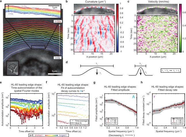
(**a–c**) Example of leading edge fluctuations extracted from a representative migrating HL-60 cell. (a) Phase contrast microscopy image from the first frame of a movie, overlaid with segmented leading edge shapes from time points increasing from blue to red in 2 s intervals. Top Inset: Magnification of the segmented leading edge between t = 0–2 s increasing from blue to red in 50 ms intervals. Bottom Inset: A de-magnified image of the whole cell at the last time point. (**b–c**) Kymographs of curvature (b) and velocity (c). Note the velocity is always positive, so no part of the leading edge undergoes retraction. (d) Schematic demonstrating a commonly observed trend between fluctuation wavelength and relaxation time. (e) Autocorrelation amplitude (complex magnitude) of the spatial Fourier transform plotted as a function of time offset from a representative cell. Each line corresponds to a different spatial frequency in the range of 0.22–0.62 µm^–1 (corresponding to a wavelength in the range of 4.5–1.6 µm) in 0.056 µm^–1 intervals. (f) Best fit of the autocorrelation data shown in (e) to an exponential decay, fitted out to a drop in amplitude of 2/e. (**g–h**) Fitted parameters of the autocorrelation averaged over 67 cells. Data from this figure can be found in Figure 1—source data 1.

Figure 1—source data 1 Source data corresponding to plots in Figure 1. See Readme for a description of the contents, and the locations of the corresponding plots in the figure.: https://cdn.elifesciences.org/articles/74389/elife-74389-fig1-data1-v2.zip
Download elife-74389-fig1-data1-v2.zip

Video 1

Download asset

posterframe for video — Segmentation overlaid onto migrating HL-60 cell.

Time lapse video representation of segmentation results shown in Figure 1a.

We estimate we were able to reliably measure fluctuations with wavelengths as small as ~650 nm, and amplitudes down to ~65 nm, by fitting the phase contrast halo around the leading edge (Figure 1—figure supplements 1–2, Materials and methods). These values should approximately correspond to 25 actin filaments at physiological spacing (Svitkina et al., 1997) and 25 actin monomers assembled into a filament lattice along the direction of motion. While our measurements of shape dynamics cannot resolve polymerization events of individual filaments, our results are consistent with the hypothesis that stochasticity in actin growth at the level of monomer addition – occurring throughout the leading edge actin network – ultimately manifests as the observed micron-scale leading edge fluctuations. In particular, kymograph analysis of curvature and velocity (Figure 1b–c) showed that relatively long-lived shape fluctuations are formed by the continual time-integration of seemingly uncorrelated and very short-lived (sub-second, sub-micron) velocity fluctuations. Because the average cell shape remains constant over time, there must be some form of feedback acting on leading edge curvature to sustain stable lamellipodial growth. These rich, measurable fine-scale dynamics therefore provide a unique opportunity to directly observe the time-evolution of leading edge maintenance. Taking advantage of our high-precision measurements, we aimed to quantitatively investigate the properties of the observed fluctuations, with the goal of determining the mechanisms by which molecular machinery at the leading edge coordinates the stochastic polymerization of individual actin filaments.

Lamellipodial stability mediated by viscous relaxation of shape fluctuations

The relaxation of fine-scale shape fluctuations back to the steady-state leading edge shape is essential for the long time scale stability of lamellipodia. As for any physical system, the nature of this relaxation reflects the system’s underlying physical properties; in this case, the characteristics of – and interactions between – actin filaments and the membrane. To provide a framework for exploration of the physical mechanisms underlying stable lamellipodial protrusion, we quantified the relaxation dynamics by performing time-autocorrelation analysis on the leading edge shape (Materials and methods). Applied in this context, this analytical technique calculates the extent to which the lamellipodium contour loses similarity with the shape at previous time points as fluctuations emerge and relax. As most material systems (actively-driven or otherwise) exhibit relaxation behavior with a characteristic wavelength-dependence (e.g. Figure 1d), we performed Fourier decomposition on the leading edge shape to separate out fluctuations at different length scales, and then performed autocorrelation analysis separately on each Fourier mode. We validated our analytical methods using simulations of membrane dynamics, for which there exists a well-established analytical theory (Materials and methods, Figure 1—figure supplement 3), and show that our results are not sensitive to an extension of our analysis to longer length and time scales (Materials and methods, Figure 1—figure supplements 4–5). Further, the membrane simulation control nicely demonstrates how visual features of curvature kymographs (e.g. Figure 1b) can be misleading (Materials and methods, Figure 1—figure supplement 3), and motivates the necessity of our more comprehensive technique.

Autocorrelation analysis revealed a monotonic relaxation of shape fluctuations at each wavelength (Figure 1e–f); the decay at every spatial scale is well-fit by an exponential form (Figure 1f), consistent with overdamped viscous relaxation. Importantly, we do not detect any increase in the autocorrelation over time, which would have appeared if there were any sustained, correlated growth of the fluctuations before they decay. This again suggests that the fluctuations arise from uncorrelated stochastic processes, such as fluctuations in actin density. A clear wavelength-dependence is observed, with shorter wavelengths decaying faster and having smaller amplitudes (Figure 1g–h). This general trend is shared by many physical systems with linear elastic constraints, such as idealized membranes (Brown, 2008) and polymers (De Gennes, 2002) freely fluctuating under Brownian motion, but can be contrasted with systems that have a dominant wavelength, as in the case of buckling or wrinkling of materials under compression (Cerda and Mahadevan, 2003). Importantly, these qualitative and quantitative properties of the leading edge fluctuations are not specific to cell type or experimental conditions (e.g. agarose overlay, ECM), as we also observe this phenomenon in fish epidermal keratocytes (Figure 1—figure supplement 6, Video 2).

Video 2

Download asset

Leading edge stability as an emergent property of branched actin growth

The rich behavior and quantitative nature of our leading edge shape fluctuation data made them ideal for comparison with physical models. In order to understand how molecular-scale actin assembly and biomechanics might give rise to the observed micron-scale shape dynamics, we aimed to reproduce this behavior in a stochastic model of branched actin network growth against a membrane (Figure 2a–c, Video 3, Materials and methods). Previous stochastic models of protrusive actin-based forces largely focused on actin polymerization against rigid obstacles (e.g. the bacterial cell wall for the Listeria comet tail Carlsson, 2001; Carlsson, 2003 or a single, flat membrane segment in models of lamellipodia Mueller et al., 2017). Expanding on this general framework, and in an approach conceptually similar to previous work simulating small (< 2 µm) patches of a lamellipodium (Schaus et al., 2007; Schaus and Borisy, 2008), we incorporated a two-dimensional leading edge with filaments polymerizing against a flexible membrane, which we modeled as a system of flat membrane segments coupled elastically to each other. The size of the membrane segments was comparable to the spatial resolution of our experimental measurements, allowing us to assay fluctuations over a similar dynamic range of wavelengths. Simulated filaments apply force to the membrane following the classic untethered Brownian ratchet formalism (Mogilner and Oster, 1996), consistent with recent experiments showing that cellular protrusions are formed by largely untethered actin networks (Bisaria et al., 2020). Designed to be as comparable as possible to our experimental data, the model incorporated experimentally measured values from the literature for the membrane tension, membrane bending modulus, and biochemical rate constants (Tables 1–2, Mogilner and Oster, 1996; Lieber et al., 2013). As we were specifically interested in identifying biophysical mechanisms regulating leading edge stability, we minimized the model’s biological complexity by including only the core biochemical elements of actin network growth dynamics: polymerization, depolymerization, branching, and capping. All filament nucleation in the model occurs through dendritic branching observed in cells to be mediated by the Arp2/3 complex (Welch et al., 1997; Svitkina et al., 1997), which catalyzes the nucleation of new ‘daughter’ actin filaments as branches from the sides of pre-existing ‘mother’ filaments at a characteristic angle of ~70° (Mullins et al., 1998; Volkmann et al., 2001; Rouiller et al., 2008). By simulating individual filament kinetics, the model captures the evolutionary dynamics of the filament network, allowing us to directly test hypothesized mechanisms for the interplay between actin network properties (e.g. filament orientation) and protrusion dynamics (Mogilner and Oster, 1996; Lacayo et al., 2007; Mueller et al., 2017; Grimm et al., 2003; Maly and Borisy, 2001; Schaus et al., 2007; Figure 2b).

Figure 2 with 3 supplements see all

Download asset Open asset

Minimal model of branched actin growth recapitulates leading edge stability and shape fluctuation relaxation.

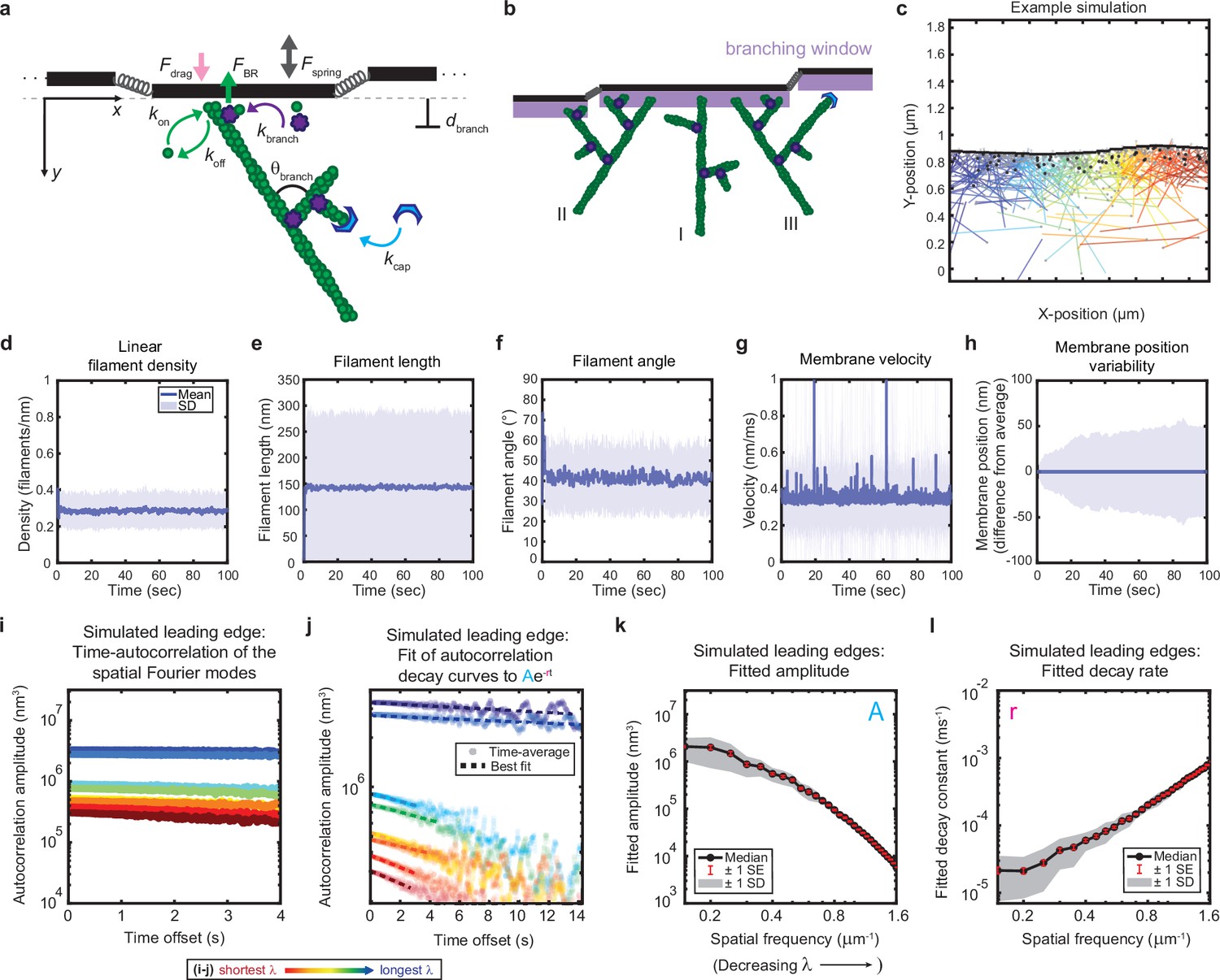
(**a–b**) Model schematic. Black lines, membrane; green circles, actin; purple flowers, Arp2/3 complex; blue crescents, capping protein. Rates: k_on, polymerization; k_off, depolymerization; k_branch, branching; k_cap, capping. θ_branch, branching angle. d_branch, branching window. Physical parameters: F_spring, forces between membrane segments; F_BR, force of filaments on the membrane (Brownian ratchet); F_drag, viscous drag. (b) Schematic demonstrating filament angle evolution. Filaments growing perpendicular to the leading edge (I) outcompete their progeny (branches), leading to a reduction in filament density; filaments growing at an angle (II and III) make successful progeny. Filaments spreading down a membrane positional gradient (II) are more evolutionarily successful than those spreading up (III). (c) Simulation snapshot: Black lines, membrane; colored lines, filament equilibrium position and shape; gray dots, barbed ends; black dots, capped ends; filament color, x-position of membrane segment filament is pushing (increasing across the x-axis from blue to red). (**d-h**) For a representative simulation, mean (solid line) and standard deviation (shading) of various membrane and actin filament properties as a function of simulation time. Note for linear filament density (d) lamellipodia are ~10 filament stacks tall along the z-axis, giving mean filament spacing of 10/density, or ~30 nm. (**i–l**) Autocorrelation analysis and fitting for a representative simulation (**i–j**) as well as best fit parameters averaged over 40 simulations (**k–l**). Data from this figure can be found in Figure 2—source data 1.

Figure 2—source data 1 Source data corresponding to plots in Figure 2. See Readme for a description of the contents, and the locations of the corresponding plots in the figure.: https://cdn.elifesciences.org/articles/74389/elife-74389-fig2-data1-v2.zip
Download elife-74389-fig2-data1-v2.zip

Figure 3

Download asset Open asset

Minimal model correctly predicts response of HL-60 cells to drug treatment.

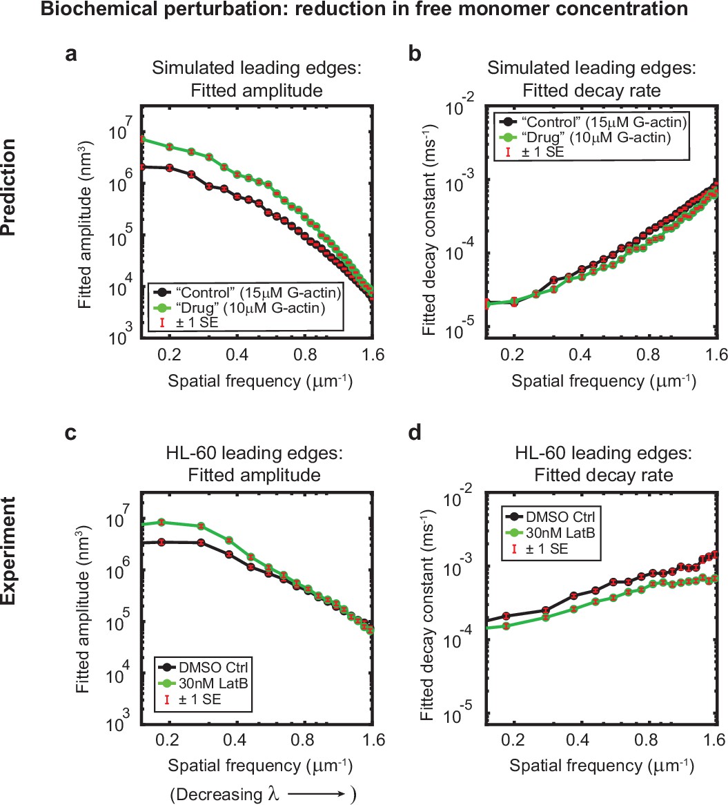
Predicted and experimentally-measured response of the autocorrelation decay fit parameters to drug treatment with Latrunculin B, plotted as in Figure 1g–h. (**a–b**) Predicted response to a reduction in the free monomer concentration (green, 10 µM G-actin) compared to the standard concentration used in this work (black, 15 µM G-actin) – medians over 40 simulations for each condition. (**c–d**) Experimentally measured behavior: DMSO control – medians over 67 cells (same data as plotted in Figure 1g–h). 30 nM Latrunculin B – medians over 34 cells. Data from this figure can be found in Figure 3—source data 1.

Figure 3—source data 1 Source data corresponding to plots in Figure 3. See Readme for a description of the contents, and the locations of the corresponding plots in the figure.: https://cdn.elifesciences.org/articles/74389/elife-74389-fig3-data1-v2.zip
Download elife-74389-fig3-data1-v2.zip

Video 3

Download asset

Table 1

Actin network growth parameters.

Parameters listed are the default used for the simulations.

Notation	Meaning	Value	Source
M	Free monomer concentration	15 µM	Cooper, 1991; Marchand et al., 1995
k_on	Polymerization rate	11∙10^–3 monomers ms^–1 µM^–1	Pollard, 1986
k_off	Depolymerization rate	10^–3 monomers ms^–1	Pollard, 1986
k_cap	Capping rate	3∙10^–3 ms^–1	~3∙10^–3 µM^–1 ms^-1 Schafer et al., 1996at 1 µM capping protein Pollard et al., 2000
k_branch	Branching rate	4.5∙10^–5 branches ms^–1 µM^–1 nm^–1	50 nm branch spacing Svitkina et al., 1997; Svitkina and Borisy, 1999;Branch rate approximated such that elongation rate / branch rate = 50 nm; k_branch = (k_on∙M∙l_m)/(50 nm∙M∙y_branch)
y_branch	Branching window length	15 nm	~3–5 protein diameters away from the membrane
θ_branch	Branching angle	70 ± 10°	Mullins et al., 1998; Volkmann et al., 2001; Rouiller et al., 2008; Blanchoin et al., 2000; Cai et al., 2008; Svitkina and Borisy, 1999
l_p	Actin filament persistence length	1 µm	Käs et al., 1996
l_m	Actin monomer length	2.7 nm	Pollard, 1986

Table 2

Physical parameters.

Parameters listed are the default used for the simulations.

Notation	Meaning	Value	Source
k_B	Boltzmann constant	0.0183 pN nm K^–1	–
T	Temperature	310.15 K	–
σ	Membrane tension	0.03 pN nm^–1	Lieber et al., 2013
κ	Membrane bending modulus	140 pN nm	Lieber et al., 2013
η_w	Viscosity of water at 37 °C	7∙10^–7 pN ns nm^–2	–
η	Effective viscosity at the leading edge	3000 η_w	~ effective viscosity of micron-scale beads in cytoplasm Wirtz, 2009
L	Leading edge length	20 µm	This work
h	Leading edge height	200 nm	Abraham et al., 1999; Laurent et al., 2005; Urban et al., 2010
Δx	Membrane segment length	100 nm	–
N	Number of membrane segments	200	–

To our great surprise, this very simple model was able to recapitulate stable leading edge fluctuations. Nascent leading edges reach steady state values for filament density, filament length, filament angle, membrane velocity, and (most importantly) membrane fluctuation amplitude within seconds, a biologically realistic time scale (Figure 2d–h). Furthermore, the steady state values obtained are in quantitative agreement with both our own experimental data and previously published measurements, with the model yielding mean values of: 0.3 filaments/nm for filament density (~30 nm filament spacing for a lamellipodium that is 10 filaments tall) (Abraham et al., 1999), ~150 nm for filament length, ~40° for filament angle (with respect to the direction of migration), ~0.35 nm/ms for membrane velocity, and ~50 nm for membrane fluctuation amplitude (Svitkina et al., 1997; Maly and Borisy, 2001; Verkhovsky et al., 2003).

As observed in the experimental measurements, simulated leading edge shape stability is mediated by an exponential decay of shape fluctuations (Figure 2i–j). Furthermore, the minimal model correctly predicts the monotonic trends of fluctuation amplitude and decay time scale with wavelength (Figure 2k–l) in a way that was not sensitive to our choices of simulation time step, membrane segment length, and overall length of the leading edge (Figure 2—figure supplements 1–3). It should be noted that the generation of the simulated data in Figure 2k–l did not involve any curve-fitting (and therefore no free parameters that could be fit) to the experimentally measured autocorrelation dynamics in order to parameterize the model. Rather, the simulated fluctuation relaxation behavior, qualitatively reproducing our experimental measurements, emerges directly from the molecular-scale actin growth model, in which all biochemical parameters were estimated from measurements in the existing literature (Tables 1–2) – leaving no free simulation parameters.

Predicting effects of drug treatment with Latrunculin B

We were interested in further assaying the predictive power of this minimal stochastic model by determining whether the output of the simulations was congruent with experimental observations under conditions that had not been tested prior to model development. As an example, we elected to test whether the model could correctly predict the response of HL-60 cells to treatment with the drug Latrunculin B, which binds to and sequesters actin monomers. Qualitatively, cells treated with Latrunculin B (Video 4) present with enhanced bleb formation and more variable leading edge shapes, in comparison with cells treated with a DMSO vehicle control (Video 5). In our model, addition of this drug can be simulated by reducing the free monomer concentration, which consequently reduces both the polymerization rate and the branching rate. At low effective doses, subtle but measurable changes to leading edge fluctuations were predicted: specifically, an increase in the amplitudes at large wavelengths, and a decrease in the decay rates across all wavelengths (Figure 3a–b). Our experimental results were consistent with these quantitative predictions; Latrunculin B-treated cells exhibited increased fluctuation amplitudes and decreased fluctuation rates over the predicted ranges (Figure 3c–d).

Video 4

Download asset

Video 5

Download asset

Geometry as the core determinant of simulated leading edge stability

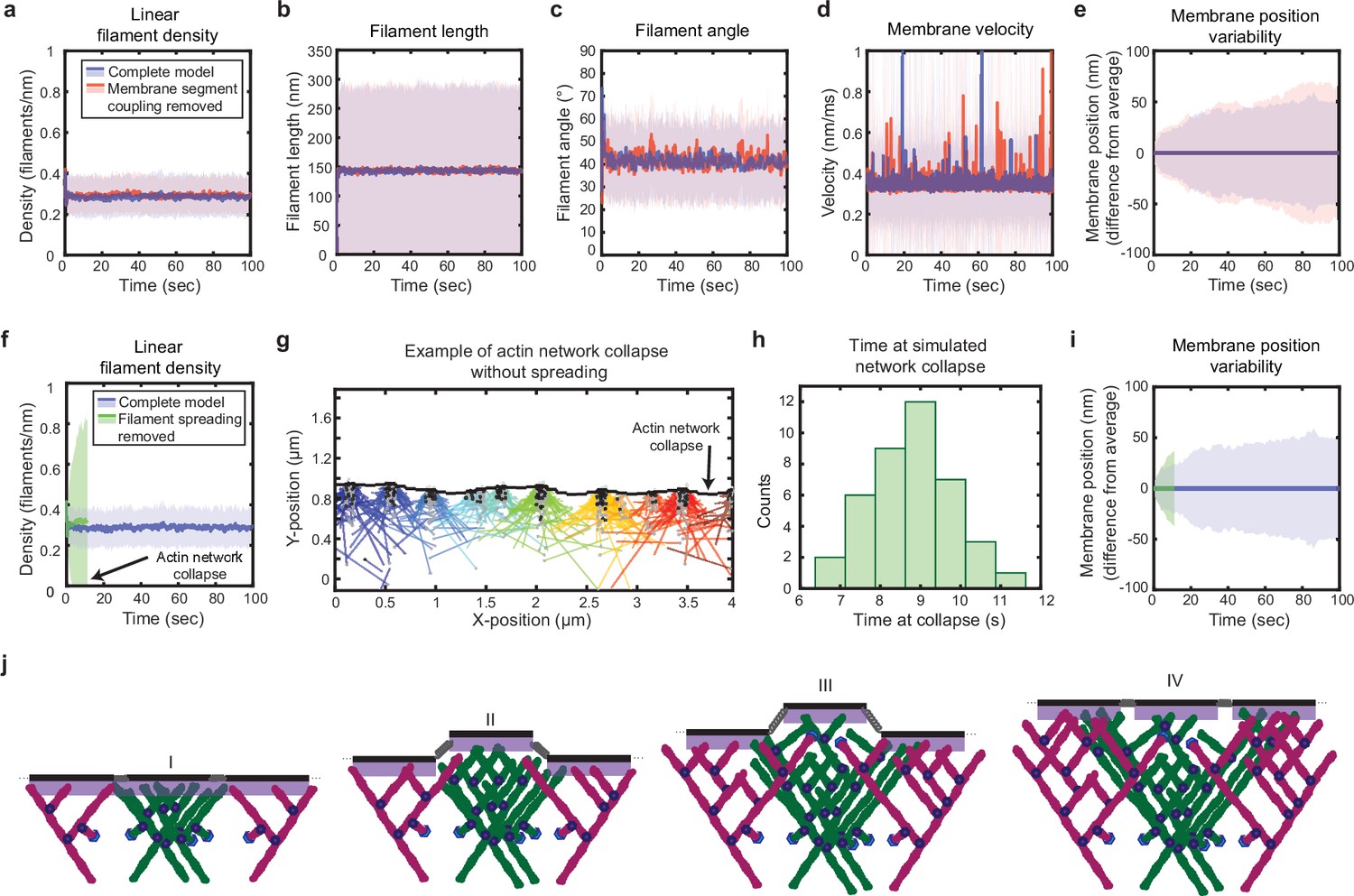
Given the success of the model in reproducing experimental results, we next wanted to determine which features of the simulation were responsible for leading edge stability and relaxation of fluctuations. The simplicity of the model allowed us to determine the stability mechanism by process of elimination, selectively removing elements of the model (Materials and methods) and determining whether stability was retained. To assay the importance of membrane tension and bending rigidity, which has been suggested to be a key factor regulating lamellipodial organization (Batchelder et al., 2011; Sens and Plastino, 2015), we simply removed the forces between the membrane segments (Figure 2a, F_spring) from the simulation (Materials and methods). Surprisingly, the coupling between the membrane segments (i.e. the effects of tension and bending at length scales larger than the size of an individual membrane segment) was completely dispensable for leading edge stability (Figure 4a–e).

Figure 4

Download asset Open asset

Simulated lamellipodial stability is governed by leading edge geometry.

(**a–e**) Comparison of leading edge properties with and without the coupling of the membrane segments by tension and bending rigidity (no coupling: *F_spring* = 0 in Figure 2a), plotted as in Figure 2d–h. (**f–i**) Comparison of leading edge properties with and without the ability of filaments to spread between neighboring membrane segments. (g) A snapshot of the simulation after filament network collapse (defined as a state where at least 25% of the membrane segments have no associated filaments). (**f,g,i**) Plots made from the same simulation. (h) A histogram of the average time to network collapse over 40 simulations. (j) Schematic representing the proposed molecular mechanism underlying the stability of leading edge shape, with time increasing from I-IV. Data from this figure can be found in Figure 4—source data 1.

Figure 4—source data 1 Source data corresponding to plots in Figure 4. See Readme for a description of the contents, and the locations of the corresponding plots in the figure.: https://cdn.elifesciences.org/articles/74389/elife-74389-fig4-data1-v2.zip
Download elife-74389-fig4-data1-v2.zip

Following a similar process of elimination, we determined that in fact only two elements were required for stability. First, as reported previously for dendritic actin network polymerization against a single stiff obstacle, it was necessary to constrain branching to occur only within a fixed distance from the leading edge membrane (Figure 2a–b) in order to maintain a steady state actin density (Carlsson, 2001). The molecular motivation for this spatially limited ‘branching window’ is rooted in that fact that activators of the Arp2/3 complex, which render Arp2/3 competent for actin filament nucleation, are typically membrane-associated proteins (Suetsugu, 2013). Second, we found that stability is inherently tied to the ability of filaments to spread laterally to neighboring membrane segments (Figure 2b II-III, Figure 4f–i). Recall that, because the branched actin network geometry causes filaments to grow, on average, at an angle relative to the membrane normal (Maly and Borisy, 2001; Verkhovsky et al., 2003), polymerizing tips spread laterally along the leading edge (Lacayo et al., 2007; Grimm et al., 2003). Removing filament spreading from the model by fixing filaments to remain associated with their nearest membrane segment at birth (Materials and methods) led to actin density divergence: network regions with low filament density eventually underwent complete depolymerization, while high-density regions continued to accumulate actin (Figure 4f–g).

These findings lead us to a simple molecular feedback mechanism for leading edge stability, based on a synergy between filament spreading and membrane-proximal branching (Figure 4j): To begin with, regions with initially high filament density come to protrude beyond the average position of the rest of the membrane, representing the emergence of a leading edge shape fluctuation (Figure 4j, I, II). This induces asymmetric filament spreading, where filaments from high-density regions can spread productively into neighboring regions (Figure 2b, II), but filaments spreading from adjacent low-density regions cannot keep up with the fast moving membrane segments (Figure 2b, III), and thus are unproductive (Figure 4j, II, III). In this way, the branched geometry inherent to dendritic actin polymerization, as well as its interaction with the shape of the membrane, naturally encodes leading edge stability (Figure 4j, IV). Thus our results directly demonstrate a ‘stability-through-spreading’ mechanism that has previously only been assumed in mean-field analytical theories (Lacayo et al., 2007; Grimm et al., 2003). Remarkably, this means that leading edge maintenance is an intrinsic, emergent property of branched actin network growth against a membrane, without requiring any further regulatory governance. Geometrical constraints imposed simply by the nature of membrane-proximal actin branching ensure that any small variations in either local actin filament density or growth rate are inherently self-correcting to regress toward the mean.

Of note, it has previously been shown that Arp2/3-mediated branching is required for lamellipodial formation in a wide variety of cell types; cells with inhibited or depleted Arp2/3 complex exhibit complete disruption of the lamellipodium shape and often switch to a different mode of migration altogether, such as filopodial motility (Fritz-Laylin et al., 2017b; Henson et al., 2015; Wu et al., 2012; Davidson et al., 2018). Indeed, HL-60s treated with the Arp2/3 inhibitor CK-666 have extremely variable leading edge shapes, characterized by long, thin filopodia-like protrusions (Video 6). Our theoretical results provide a mechanistic interpretation for this striking phenomenon, suggesting that the vital lamellipodial maintenance role of Arp2/3-mediated branching stems from its ability to mediate efficient filament spreading and equilibration of actin density fluctuations, purely because the daughter filament always grows at an angle distinct from its mother.

Video 6

Download asset

Optimal suppression of fluctuations by the highly conserved ~70° branching angle

Given the essential contribution of branched network geometry to the stability of the simulated leading edges, we reasoned that variations in the branching geometry alone might have a significant effect on leading edge fluctuations. We therefore performed simulations to determine the effects of changing the average branching angle and branching angle variability on filament orientation, filament density, and leading edge fluctuation fit parameters (Figure 5). In this context, we highlight the distinction between the branching angle, θ_br (i.e. the angle of a daughter filament relative to its mother), and the filament angle or orientation, θ_f (i.e. the angle of a filament relative to the direction of migration) (Figure 5a, inset). Due to the sterotypical branching angle, θ_br, there is a direct correspondence between the orientation, θ_f^mother, of a mother filament and the orientation, θ_f^daughter, she passes on to her daughter branches. Our simulations are thus, in effect, selection assays, as mother filaments compete to stay within the fixed branching window, spawn daughter branches, and thus pass down their angle to their progeny (Maly and Borisy, 2001; Schaus et al., 2007). For example, when filaments are initialized with a random orientation, and the branching angle is fixed (i.e. there is no variability in the branching angle), only a handful of the initial filament angles (θ_f) survive until the end of the simulation (Figure 5a). The surviving, successful filament angles are narrowly and symmetrically distributed around one half of the branching angle (Figure 5a–c). This optimal filament angle allows mother and daughter filaments to branch back and forth symmetrically about the membrane normal, such that mother filaments do not out-compete their progeny (as has been described previously) (Maly and Borisy, 2001; Schaus et al., 2007; Schaus and Borisy, 2008; Figure 2b).

Figure 5

Download asset Open asset

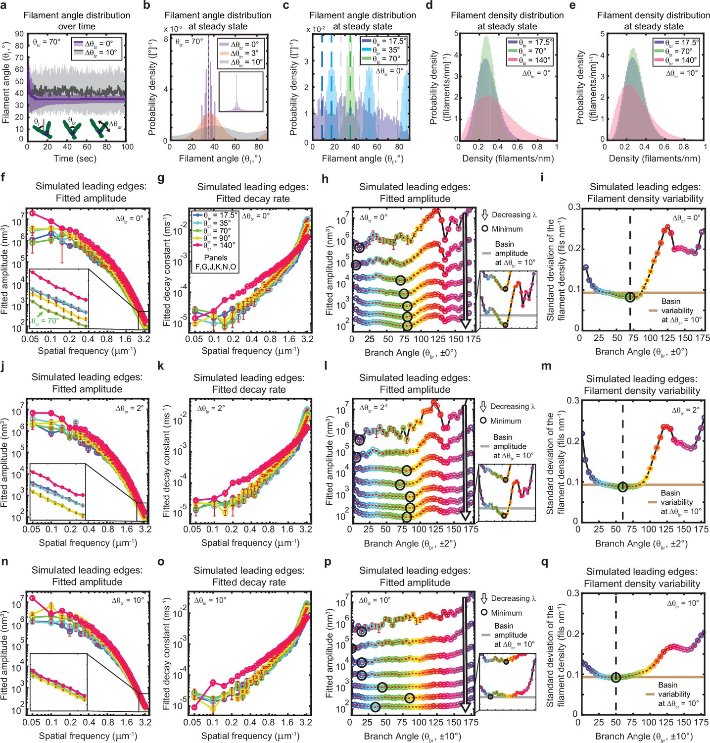
The genetically-encoded Arp2/3-mediated branching angle is optimal for suppressing leading edge fluctuations.

(**a–c**) Time course (a) and steady state distribution (**b–c**) of the filament angle (θ_f) for simulations with various branching angle standard deviations (Δθ_br), (**a–b**) and means (θ_br), (c). Dashed lines represent θ_br/2 plus integer multiples of θ_br. (**d–e**) Steady state filament density distribution as a function of the mean branching angle in the context of Δθ_br=0° (d) and Δθ_br=10° (e). (**a–b, d–e**) Results from a representative simulation for each condition. (c) Data integrated over 40 simulations. (**f–q**) Predicted response of leading edge fluctuations and filament density variability to changes in the branch angle and branch angle variability, medians over 40 simulations for each condition. Red error bars – standard error. Color map is identical for panels c-q. (**h,l,p**) Fitted amplitude as a function of branch angle, where each line represents a different spatial frequency, increasing from 0.2 to 3.2 µm^–1 in intervals of 0.5 µm^–1. Insets have identical x-axes to main panels. (**i,m,q**) Standard deviation of the filament density at steady state plotted as a function of branch angle. Note the x- and y-axes limits in (**f–g, j–k, n–o**) are expanded compared to the equivalent panels in Figures 1—3. Data from this figure can be found in Figure 5—source data 1.

Figure 5—source data 1 Source data corresponding to plots in Figure 5. See Readme for a description of the contents, and the locations of the corresponding plots in the figure.: https://cdn.elifesciences.org/articles/74389/elife-74389-fig5-data1-v2.zip
Download elife-74389-fig5-data1-v2.zip

In living cells, branching is mediated by the Arp2/3 complex, which has been experimentally measured to form highly regular and sterotyped branches at ~70° (Mullins et al., 1998; Volkmann et al., 2001; Rouiller et al., 2008). Intriguingly, this protein complex is highly conserved (Welch et al., 1997), with measurements of the branching angle in a wide variety of species, including protists (Mullins et al., 1998; Volkmann et al., 2001; Rouiller et al., 2008; Blanchoin et al., 2000), yeast (Rouiller et al., 2008), mammals (Rouiller et al., 2008; Blanchoin et al., 2000; Cai et al., 2008), and amphibians (Svitkina and Borisy, 1999), using various experimental techniques (platinum replica electron microscopy, cryo-electron microscopy, and total internal reflection microscopy), all falling within the range of 67–78° (± 2–13°). The high degree of conservation hints that this specific angle might carry some functional optimality, but the question has not been addressable experimentally; due to the lack of naturally occuring Arp2/3 variants with a substantially different branching angle, an alternative branching structure would hypothetically have to be designed do novo, presumably by altering the protein interaction interface by which the Arp2/3 complex binds to the side of a mother filament (Volkmann et al., 2001). We thus sought to explore the possible functional significance of this conserved angle using our minimal stochastic model. Excitingly, we found that in simulations with no branch angle variability, a 70–80° branching angle was optimal for minimizing both actin density fluctuations (Figure 5d and i) and leading edge fluctuation amplitudes for wavelengths smaller than ~2 µm (Figure 5f and h). These smoothing effects are therefore predicted to be relevant within the experimentally-measurable range of wavelengths (between ~0.7 µm and ~2 µm), but are most beneficial for the smallest wavelengths resolved by our simulations (down to ~0.3 µm) – closest to the length scales of individual filament polymerization. Overall, these results provide tantalizing mechanistic insight into the long-standing question of why the characteristic branching angle is so ubiquitous.

Heritability of filament orientation (i.e., the extent to which mother filament orientation determines the orientation of the daughters) is set by the degree of variability in the branching angle (which, in turn, reflects the influence of thermal fluctuations). Perhaps unsurprisingly, decreasing this orientational heritability significantly reduces the dependence of fluctuation amplitude and filament density variability on the branching angle (Figure 5j–q), and thereby counteracts the beneficial effect of the optimal angle on leading edge fluctuations. Introducing a branch angle variability of ±2° (on the lower end of the experimentally-measured values) broadens the range of near-optimal branch angles but maintains the optimum at ~70–80° (Figure 5j and l), while introducing a variability of ±10° (on the higher end of the measured range) completely removes the optimum (Figure 5n and p). In both cases, increasing the branch angle variability increases the minimum possible fluctuation amplitude (Figure 5h, l and p – insets) and filament density variability (Figure 5i, m and q), representing a decrease in the noise-suppression capabilities of the system. Overall, these results provide strong support for the idea that actin network geometry is not only essential for leading edge stability, but also plays a major role in determining the fundamental limits of smoothness in lamellipodial shape.

Discussion

The emergence of robust collective behaviors from stochastic elements is an enduring biological mystery which we are only beginning to unravel (Huang et al., 2016; Battich et al., 2015; Chang and Marshall, 2017; Mohapatra et al., 2016; Raj and van Oudenaarden, 2008; Gray et al., 2019; Oates, 2011). The apparent dichotomy in actin-based motility between the random elongation of individual filaments and the stable formation of smooth and persistent higher order actin structures such as lamellipodia exemplifies this enigma, and provides an avenue toward understanding general strategies for noise suppression in biological systems.

In recent years it has become clear that perturbation-free experiments which examine fluctuations around the mean at steady state (in contrast to probing the change in the mean due to a perturbation) can be a powerful tool for understanding noisy systems (Welf and Danuser, 2014). In this work, application of that principle in combination with high-precision measurements, quantitative analytical techniques, and physical modeling led to the surprising revelation that the suppression of stochastic fluctuations naturally emerges from the interactions between a growing actin network and the leading edge membrane, with no additional feedback required. Our insights into the molecular mechanisms mediating lamellipodial stability were largely enabled by experimentally measuring micron-scale leading edge shape dynamics and comparing them to a molecular-scale actin network growth model that correctly predicts this emergent behavior (as well as many other experimentally-measured features of lamellipodial actin networks). Ultimately, we hope our results inspire future experimental work to directly measure the nanometer-scale interactions predicted by our simulations, which may be accomplished using super-resolution imaging of actin dynamics in vivo or in an in vitro reconstitution of lamellipodial protrusion (i.e. branched polymerization of actin driving the motion of a flexible barrier).

The model developed in this work provides an understanding of the basic biophysical mechanisms underlying lamellipodial migration. Of course, living cells are home to array of additional complexities which are likely to further modulate leading edge fluctuations and stability, and our model may provide a framework for future exploration of such effects across diverse cell types and experimental conditions. Cells migrating in vivo inevitably experience a much more challenging and dynamic environment, in which additional feedback mechanisms will almost certainly be required for the maintenance of polarized migration. The simplicity and biophysical realism of our modeling framework should make it particularly well-suited for future studies focused on predicting and understanding the effects of additional potential feedback mechanisms, including tethering (Mogilner and Oster, 2003; Soo and Theriot, 2005; Alberts and Odell, 2004; Kuo and McGrath, 2000), a limiting monomer concentration (Mullins et al., 2018), force-dependent branching (Risca et al., 2012; Parekh et al., 2005; Chaudhuri et al., 2007), and regulation by curvature-sensing proteins (Tsujita et al., 2015; Zhao et al., 2011). Further, this computational model might be useful for exploring the effects of various extracellular forces, such as those produced by obstacles or variations in matrix density, or intracellular forces, such as those produced by hydrostatics. We also note that a certain degree of biochemical signaling is implicit in our model in the form of biochemical rate constants that are invariant in time and space; this property relies on signaling networks to maintain uniform gradients of actin-associated molecules (Devreotes et al., 2017). How local biochemical control (or lack thereof) over these rate constants might affect leading edge fluctuations remains an interesting avenue for future investigation, both theoretically and experimentally.

The defining characteristic and major advance of our model was the explicit inclusion of both the evolutionary dynamics of the actin network and its interaction with the two-dimensional geometry of the leading edge. By selectively removing elements of the model, we determined that lateral filament spreading, combined with a fixed branching window, is indispensable for leading edge stability. This highlights the crucial role in lamellipodial maintenance of the branched structure of actin networks, wherein each daughter filament inherits angular information from its mother. Our further investigations into the evolutionary properties of actin network growth revealed that a ~70–80° branch angle maximally suppresses fine-scale actin density and leading edge shape fluctuations, showing for the first time that Arp2/3-mediated branching imparts optimal functionality, as was long hypothesized based on strong sequence, structural, and functional conservation throughout the eukaryotic tree of life. It is interesting to note that the evolutionarily-conserved branching angle that we find maximally suppresses leading edge fluctuations appears not to be the same angle that optimizes the polymerization velocity of single filaments – predicted to be a broad angle closer to ~90–100° (and quite load-dependent) in the low-load regime (Mogilner and Oster, 1996). This contrast suggests that evolutionary selection acts at the level of actin network properties, rather than force production by individual filaments.

Returning to the broader question of how noisy biological systems control for stochasticity, we find that stability in the case of lamellipodial dynamics is inherently encoded by the geometry of branched actin network growth. It will be interesting to see whether similar principles hold for other cytoskeletal structures with clear geometric constraints, such as endocytic pits, the cytokinetic ring, and the mitotic spindle.

Materials and methods

HL-60 cell culture and differentiation

Request a detailed protocol

HL-60 cells were cultured as described previously (Millius and Weiner, 2009; Garner et al., 2020). In brief, cells were maintained at a density of 0.1–1 x 10⁵ cells/mL by passaging every 2–3 days into fresh RPMI media supplemented with 10% heat-inactivated fetal bovine serum and antibiotics/antimycotics. Supplementation with 1.57% DMSO was used to differentiate the cells into a neutrophil-like state. Cells were subsequently extracted for experiments at 6 days post-differentiation. Our HL-60 cell line was obtained from Orion Weiner’s lab at UCSF, who originally received them from Henry Bourne’s lab at UCSF. The identity of this suspension cell line was confirmed based on the behavior of the cells, including differentiating into a neutrophil-like state upon exposure to DMSO that exhibits characteristic phenotypes for substrate adhesion, rapid migration, and elongated morphology. HL-60s are not listed as a misidentified cell line on the Register of Misidentified Cell Lines. The cell line tested negative to mycoplasma contamination.

Under-agarose motility assays with HL-60s

Request a detailed protocol

Differentiated HL-60 cells were plated on fibronectin-coated coverslips and then overlaid with a 1% agarose pad containing 1 nM fMLP (to enhance migratory behavior), as described previously (Garner et al., 2020). Microscopy of the migrating cells was performed at 37 °C, using transmitted light to image phase contrast on an epifluorescence microscope at ×100 magnification (100 × 1.45 NA Plan Apo oil objective, Nikon MRD31905). A more detailed description of our microscopy system can be found in previous publications (Garner et al., 2020). For treatment with Latrunculin B or CK-666, the drug was embedded into the agarose pad by adding the drug to the unpolymerized agarose pad solution before gelling (at the same time as adding fMLP), such that drug treatment begins when cells are overlaid with the agarose pad and is maintained throughout imaging. Cells were imaged at 45 min post-plating. Drugs were first diluted down to 1000 X in DMSO, then added to the agarose solution at a dilution of 1:1,000 (for a final concentration of 30 nM for Latrunculin B and 100 μM for CK-666), giving a final DMSO concentration in the pad of 0.1%. Controls were performed by adding 0.1% DMSO to the agarose pad alone.

Keratocyte isolation and motility assays

Request a detailed protocol

Keratocytes were cultured from wild-type zebrafish embryos at 2 days post-fertilization as described previously (Lou et al., 2015). Briefly, zebrafish embryos were collected at 2 days post-fertilization, dechorionated, and anesthetized using tricaine. To dissociate the keratocytes, dechorionated fish were then washed in PBS, incubated in Cell Dissociation Buffer for 30 min at 4 °C, incubated in a solution of 0.25% trypsin and 1 mM EDTA for ~15 min at 28 °C, and then incubated in fetal bovine serum to quench the trypsin. From this point on, cells were maintained in antibiotic and antimycotic to deter microbial growth. The keratocyte-rich supernatant was then concentrated by centrifugation at 500 g for 3 min. Keratocytes were then plated on collagen-coated coverslips and incubated at room temperature for ~1 hr to allow cells to adhere. Once adherent, the supernatant was exchanged for imaging media (10% fetal bovine serum in L-15) and allowed to incubate another 15 min at room temperature before imaging. The keratocytes were imaged at 28 °C under similar conditions as those used for HL-60 cells. Data included in Figure 1—figure supplement 6 represent cells from a single coverslip. Experiments were approved by University of Washington Institutional Animal Care and Use Committee (protocol 4427–01).

Image segmentation

Request a detailed protocol

Most segmentation algorithms penalize curvature in the contour in order to reduce the noise in the fitting algorithm (Seroussi et al., 2012). However, this runs the risk of introducing artificial correlations and structure into the data. For example, a spring-like curvature penalty would artificially make fluctuations appear to be stretch-dominated. Therefore, we performed the following custom segmentation algorithm to avoid these potential artifacts (Figure 1—figure supplement 1). Phase contrast time-lapse videos were manually aligned to the direction of motion of the cell, such that each cell migrates up the y-axis on an x-y coordinate system (Figure 1—figure supplement 1a, b). The videos were then cropped to isolate the cell leading edges and exclude the cell body, for easier segmentation. If the cell migrates up the y-axis, this means every image pixel along the x-axis has an associated leading edge position along the y-axis. A leading edge y-position was assigned to each x-axis pixel independently of knowledge about neighboring x-axis pixels, to avoid injecting the artifacts discussed above. A manual segmentation was performed for the first time point in each movie. A custom, automated segmentation algorithm written in MATLAB then performed a line scan of the phase contrast intensity along the y-axis separately for each pixel along the x-axis. For each line scan, the algorithm performs a local search for the leading edge position, constrained to be within a fixed number of pixels from either the manual segmentation (for the first time point) or the previous time point (for subsequent timepoints). The leading edge position is defined as the midpoint between the brightest phase intensity (phase halo) and the point of steepest intensity gradient (transition from phase halo to phase-dense cytoplasm).

Preparation of the curvature and velocity kymographs

Request a detailed protocol

The curvature and velocity kymographs (Figure 1b–c, Figure 1—figure supplement 3) were prepared using custom MATLAB code. Curvatures are calculated as the inverse radius of the best-fit circle corresponding to a 30 pixel-wide (~1.5 µm) region about each position. The most prominent fluctuation events seen in the curvature kymographs (Figure 1b, Figure 1—figure supplement 3) somewhat correspond to (but do not exactly match) the length of the fitting window. For example, the simulated and experimental data shown in Figure 1—figure supplement 3 were fit using the same ~1.5 µm fitting window and have similar apparent ‘dominant wavemodes’ of ~3 μm, or twice the fitting window. However, despite being fit with the same fitting window, the simulated data has an observably smaller apparent ‘dominant wavemode’ than the experimental data. Velocities were calculated as the distance traveled over 250ms (five 50ms timepoints) non-overlapping windows.

Processing of segmented cell shapes for autocorrelation analysis

Request a detailed protocol

Kymographs of curvature and velocity such as those shown in Figure 1b–c, while helpful to obtain a qualitative sense of the fluctuation data, are visually dominated by the largest size-scale features of the leading edge. They thus offer an incomplete description of the shape fluctuations (Ma et al., 2018) – notably de-emphasizing the fine-scale features that are the subject of this study. Further, curvature kymographs emphasize features that are approximately the same size as the fitting window, and fail to pick up fluctuations at different size scales. To perform a quantitative analysis which faithfully captures fluctuations at all size scales, we choose to perform Fourier decomposition on the leading edge shape, and analyze the dynamics of each wavemode separately. As cells migrate, their global leading edge shape undergoes long timescale changes, such as variations in width, large-scale curvature, or slight turning of the cell, which can dominate the Fourier amplitudes and the subsequent autocorrelation signal. As we are most interested in extracting the fine-scale fluctuations, we performed background subtraction on the segmented leading edge shapes (Figure 1—figure supplement 2). To do this, we defined the ‘background’ leading edge shape as the contour after smoothing (by the lowess method, using a span of 7 μm). This rather large smoothing window was chosen specifically to preserve fine-scale features. The background-subtracted y-position is thus defined as the difference between the segmented leading edge and its smoothed counterpart. This process removed the large-scale features of the leading edge. We next wanted to remove the long-timescale features of the leading edge, so we also subtracted the time-averaged background-subtracted y-position for each x-pixel. Altogether, these pre-processing steps maintained the features of interest in the curvature kymograph (Figure 1—figure supplement 3). After performing background subtraction, we still needed to control for changes in leading edge width over time. The wavelengths represented in the Fourier transform are defined as λ = L/n, where L is the length of the leading edge, and n is an integer from 0 to one half the number of pixels. If the leading edge length were to vary over time, then so would the wavelengths, making it impossible to track the behavior of a single wavelength fluctuation over time. We thus cropped the dataset along the x-axis to include only pixels which contain the cell for all timepoints in the video, thereby extracting a fixed-length leading edge subset for further analyses.

Autocorrelation analysis and fitting

Request a detailed protocol

Autocorrelation analysis and fitting were performed separately for each cell and simulation. For experimental data, the entire video was analyzed. For simulated data, analysis was only performed on the time points after the simulation had reached steady state, for which we used a conservative cut-off of 10 s (see Figure 2d–h). To separate out fluctuations at different length scales, we first performed a spatial Fourier transform on the leading edge shape. Referencing the coordinate system defined in Figure 2a, the pixels (experiments) or membrane segments (simulations) are equally spaced in the x-direction, allowing us to perform a one-dimensional Fourier transform (MATLAB fft() function, which assumes periodic boundary conditions) on the y-positions of a segmented leading edge for each time point. We then normalize the Fourier transform by a factor of dx/ $\sqrt L$ , where dx is the pixel/membrane segment size and L is leading edge length. This normalization preserves the variance and accounts for the pixel size. To measure the fluctuation relaxation, we calculated the time-averaged autocorrelation (A_n(τ) = < Y_n(t+τ)∙Y_n*(t) > _t, using non-overlapping windows in t) of each Fourier mode amplitude. The autocorrelation function extracted from this analysis contains complex elements of the form A = a + ib. We performed all plotting and fitting on the complex magnitude (sqrt (a² + b²)) of the autocorrelation function, which is most representative of the total autocorrelation.

Note that because we are plotting the complex magnitude (which is always positive), the autocorrelation plots shown in Figures 1e–f ,–2i–j are expected to decay to some non-zero background noise window, rather than to zero. Indeed, the membrane simulation control (see Validation of autocorrelation analysis implementation), which is predicted to have a purely exponentially-decaying autocorrelation function, also shows a decay to a noise window at long times (Figure 1—figure supplement 4). We fit each Fourier mode time-autocorrelation to the exponential decay function described in the main text (Figure 1f), fitting ln(|A_n(τ)|) vs τ to a line using MATLAB’s polyfit function, to extract fit parameters for each cell and simulation. Each curve was fit out to a drop in the amplitude by a factor of e/2, or at least 10 points. To average fit parameters over many cells, we controlled for cell-to-cell variability in leading edge length by binning the parameters by spatial frequency, and then calculating summary statistics separately for each bin.

The spatial background subtraction performed on the leading edge shape (discussed in Materials and methods: Processing of segmented cell shapes for autocorrelation analysis) was necessary to extract the fine-scale shape fluctuations studied in this work. This background subtraction is expected to remove fluctuations with wavelengths larger than ~7 µm (i.e. reduce their amplitude to zero). For this reason, only wavelengths less than 7 µm are plotted in Figure 1e–h. We note that it is possible that fluctuations with wavelengths less than, but near 7 µm might also have slightly reduced measured amplitudes (i.e. the shape of the curve in Figure 1g may artificially level off at low spatial frequency). However, any such effect would be performed uniformly in time, and therefore is not expected to affect the measured temporal dynamics (Figure 1h). Indeed, when we extend the span of our background subtraction by ~50% (up to 10 μm), we find that only the amplitude of the largest mode is altered (slightly increased) and the measured relaxation timescales are not affected (Figure 1—figure supplement 5).

Validation of autocorrelation analysis implementation

Request a detailed protocol

To validate our autocorrelation method, we analyzed control simulations of a membrane freely fluctuating under Brownian motion in the absence of actin, and showed it recapitulates predictions from analytical theory for this system (Figure 1—figure supplement 3). These simulations were performed exactly as in the leading edge simulations, using the same parameters, but without actin. The equation of motion used for membrane segments in the control simulations, as well as a derivation of the associated autocorrelation function, can be found in Appendix 2.4.4: Choice of timestep. Interestingly, the curvature kymographs of these control simulations exhibit striking visual features reminiscent of instabilities, dominant wavemodes, or oscillations – and yet such effects are absent from this system by definition (which we confirm quantitatively using our autocorrelation method, Figure 1—figure supplement 3). This suggests that similar features in the experimentally-measured curvature kymograph are also not indicative of instabilities, dominant wavemodes, or oscillations, which we confirmed by autocorrelation analysis.

Modeling

Request a detailed protocol

Here, we briefly describe the geometry and major elements of the model. Please see the Appendix for a detailed description of the model and Tables 1 and 2 for a list of the chosen parameters. A simulated patch of leading edge was modeled by a branched network of actin filaments stochastically polymerizing towards a 2D strip of membrane, subject to periodic boundary conditions. The 2D strip was discretized as membrane segments that are fixed in position along one axis and move only along the direction of motion of the simulated cell. Stochastic, fixed time step Brownian dynamics simulations, implemented with custom MATLAB code, were performed to update the membrane position and actin network properties. Actin network growth evolved from constant rate Poisson processes for polymerization, depolymerization, branching, and capping. Once polymerized, filaments were fixed in position at their branch point of origin (in the lab frame of reference), and did not undergo retrograde flow (i.e. translation of the filament position opposite the direction of migration) or translational diffusion. The membrane strip was subject to forces of bending and stretching, drag from fluid viscosity, as well as the force of actin (Mogilner and Oster, 1996; Peskin et al., 1993; Carlsson, 2001). Filaments apply force to the membrane segments according to the untethered Brownian ratchet formalism (Mogilner and Oster, 1996), in which filament pointed end positions are assumed to be rigidly connected to the network (via their branch point of origin) and their barbed end positions are able to freely fluctuate. As previously, we ignore the possibility of filament buckling due to the fact that lamellipodial filaments exist in a sufficiently low-load, high branch density regime (Mogilner and Oster, 1996), and experimental evidence shows no indication of buckling (Svitkina et al., 1997). We expanded this formalism (which previously only considered filament fluctuations perpendicular to the filament’s long axis) to include all fluctuations of the filament along the filament’s short and long axes. Each filament pushes the membrane segment that spans the growing tip’s x-position. We note that the filament angles used to determine the filament forces on the membrane and presented throughout this work are always calculated relative to the global average direction of motion of the leading edge, rather than the local average membrane normal (a simplifying approximation necessitated by the discrete geometry and motivated by the shallow curvatures exhibited by cell leading edges). Control simulations were run to verify that the leading edge fluctuation behavior described in this work was not dependent on the temporal discretization (i.e. simulations were run with sufficiently small timesteps to resolve the fastest dynamics, Figure 2—figure supplement 1), spatial discretization (i.e. simulations were run with sufficiently short membrane segments to resolve the smallest length scales at which there is significant bending, Figure 2—figure supplement 2), or leading edge length (i.e. the periodic boundary conditions were implemented correctly, such that a simulated small patch of leading edge behaves identically to an equivalently sized portion of a larger simulated patch of leading edge, Figure 2—figure supplement 3). In cases where membrane tension and bending rigidity were removed, these forces were simply not calculated in the simulation (Figure 4a–e). To remove filament spreading, we modified how the filament position was updated upon addition of a monomer in order to maintain the growing filament tip’s x-position. Addition of monomers contributed only to changes in the barbed-end y-position, leaving the x-position intact, while updating the filament length correctly (effectively sliding the pointed end x-position backwards, rather than advancing the barbed end x-position forwards, Figure 4f–i).

Appendix 1

Detailed description of the model

In this section, we outline the main features of the model and reference the Detailed Derivations for more detailed derivations.

Model geometry

Given the flat structure of lamellipodial protrusions, we considered leading edge dynamics in two dimensions. In cartesian coordinates, the cell migrates in the x-y plane along the y-axis and maintains a fixed leading edge height of 200 nm along the z-axis. The leading edge membrane was modeled as a 2D strip that restricts bending and stretching in the x-y plane and is perfectly flat along the z-axis. We discretized the membrane such that a 20 μm leading edge membrane was modeled as 200 flat, rectangular segments (each 100 nm in length along the x-axis and 200 nm in height along z-axis) whose surface normal is fixed to lie along the y-axis. The membrane is implented using a Monge parameterization, such that these membrane segments are fixed in position along the x- and z-axes and move only along the y-axis (the direction of motion of the simulated cell).

Updating the membrane position

The membrane segments are assumed to move in a viscous medium at low Reynolds number, with drag force $F_{d r a g} = - γ \frac{\partial y}{\partial t}$ and Stoke’s drag coefficient $γ = 6 π η r$ , where r is the membrane segment length (x-axis) and $η$ is the dynamic viscosity of water. The membrane also acts under the forces of membrane bending and stretching ( $F_{S / B}$ , see Appendix section 1.3), and Brownian ratchet forces by the actin filaments ( $F_{B R}$ , see Appendix section 1.4). This gives us the following equation of motion.

\sum F = 0 = - γ \frac{\partial y}{\partial t} + F_{S / B} + \sum_{n = 1}^{N_{f i l}} F_{a c t i n}^{n}

Brownian dynamics simulations, implemented with a 4th order Runge-Kutta algorithm, were performed to update the membrane segment positions. Thermal fluctuations of the membrane were ignored in this implementation, as thermal fluctuations of the (much stiffer) actin filaments dominate the membrane’s motion as well as monomer incorporation into the actin network (Mogilner and Oster, 1996). See Appendix Detailed Derivations IV for a discussion of the numerical approximations included in the simulations.

Forces of membrane bending and stretching

The simulated leading edge membrane acts under the energetic constrains of stretching and bending, characterized by the experimentally measurable parameters of membrane tension ( $σ$ , $p N \cdot n m^{- 1}$ ) and bending modulus ( $κ$ , $p N \cdot n m$ ), and using the following energy functional:

\begin{array}{ll} E_{S / B} & = \int \int \frac{σ}{2} {(\frac{\partial y}{\partial x})}^{2} + \frac{κ}{2} {(\frac{\partial^{2} y}{\partial x^{2}})}^{2} d x d z \\ = h \int \frac{σ}{2} {(\frac{\partial y}{\partial x})}^{2} + \frac{κ}{2} {(\frac{\partial^{2} y}{\partial x^{2}})}^{2} d x \end{array}

where $h$ is the height of the leading edge in the z-dimension, $\frac{\partial y}{\partial x}$ is extension of the membrane (i.e. an increase in contour length), and $\frac{\partial^{2} y}{\partial x^{2}}$ is curvature in (bending of) the membrane. The force of membrane stretching and bending on a single membrane segment ( $F_{S / B}$ ) is defined as the free energy gained by movement of the segment ( $s e g$ ), and takes the following form… (See Detailed Derivations I for a derivation of the functional derivative and resulting force.)

\begin{array}{ll} F_{S / B} & = - \int_{s} e g \frac{δ E_{S / B}}{δ y} d x \\ = σ_{eff} \frac{\partial^{2} y}{\partial x^{2}} - κ_{eff} \frac{\partial^{4} y}{\partial x^{4}} \end{array}

Actin filament Brownian ratchet forces

Actin filaments constantly undulate due to thermal fluctuations, bending and stretching to sample their conformational space. The presence of the membrane restricts fluctuations of the filament past the membrane, presenting an entropic cost and a reduction in the free energy of the filament. The force of the filament exerted on the membrane segment, $F_{a c t i n}$ , can therefore be calculated as the gain in free energy, G, by an infinitesmal movement of the membrane position, $ξ$ :

G = - k_{B} T \log Z_{c o n f}

F_{a c t i n} = {\frac{\partial G}{\partial ξ} |}_{ξ = 0}

The partition function, $Z_{c o n f}$ , determined by the energetic cost of bending the filament, $E_{b e n d}$ , defines the conformational landscape. A few considerations must be made to determine the partition funciton in our system. Each filament applies force only to the membrane segment under which the filament’s barbed (growing) end equilibrium position sits, making the approximation that each membrane segment acts as an infinite wall past which filament fluctuations are blocked. Given this assumption, the membrane only restricts filament fluctuations along the y-axis. The partition function is therefore integrated over all x-positions, but only the subset of y-positions where the filament is not restricted by the membrane. With these considerations in mind, we arrive at our partition function: (See Appendix Detailed Derivations II for a derivation of the filament bending energy and Detailed Derivations III for the derivation of the force).

Z_{c o n f} = \int_{- \infty}^{\infty} \int_{0}^{\infty} e^{- β E_{b e n d}} d y d x

where y is measured relative to the membrane surface and $β = \frac{1}{k_{B} T}$ . The final equation for the force of a filament on the membrane becomes…

F_{a c t i n} = \frac{k_{B} T e^{- \frac{1}{2} {\bar{κ}}_{Eff} y_{0}^{2}}}{\int_{0}^{\infty} e^{- \frac{1}{2} {\bar{κ}}_{Eff} {(y - y_{0})}^{2}} d y}

where y₀ is the equilibrium filament position measured relative to the membrane surface (the filament pokes through the membrane for $y_{0} < 0$ ) and

{\bar{κ}}_{Eff} = (\frac{{\bar{κ}}_{∥} {\bar{κ}}_{⟂}}{{\bar{κ}}_{⟂} c o s^{2} (θ) + {\bar{κ}}_{∥} s i n^{2} (θ)})

and ${\bar{κ}}_{⟂} = \frac{3}{L^{2} N}$ , ${\bar{κ}}_{∥} = \frac{16}{L^{2} N^{2}}$ , and $N = \frac{L}{l_{p}}$ for a filament with length L and persistence length l_p at an angle $θ$ relative to the membrane segment normal.

Actin network dynamics

Actin network dynamics including polymerization, depolymerization, branching, and capping were assumed to be independent, constant rate Poisson processes. The choice of rates are described in their respective sections below. For a given time step of $Δ t$ and rate $r$ , the probability of an event happening during any given time step is…

p = 1 - e^{- r \cdot Δ t}

where $e^{- r \cdot Δ t}$ is the probability that the event did NOT take place within a time step of $Δ t$ . A random number generator was used to determine which processes occurred in each time step. In particular, a random number was chosen between 0 and 1. If the random number lied below the probability $p$ , then the event occured. For each simulation the random number generator was seeded with a unique, semi-random number, based on the current time.

Polymerization and depolymerization

The rate of polymerization was assumed to be $r_{o n} = k_{o n} \cdot M \cdot_{g a p^{'}}$ , where $k_{o n}$ is the rate of polymerization per free monomer concentration in $m o n o m e r s m s^{-} 1 μ M^{- 1}$ , M is the free monomer concentration in $μ M$ , and $p_{g a p}$ is the probability that enough space opens up in between the filament tip and the membrane to add a monomer (such that the polymerization rate far away from the membrane is $r_{(y = \infty)} = k_{o n} \cdot M$ ). Previously, it was determined that this probability is set by thermal fluctuations of the filament (Mogilner and Oster, 1996). In other words, the probability of adding a monomer is determined by the probability that thermal fluctuations, by chance, overcome the bending and stretching energies of the filament and bend the filament tip away from the membrane enough to open up a space of sufficient size to add a monomer. Given a monomer width $Δ$ , the probability of adding a monomer is…

p_{g a p} = \frac{\int_{Δ}^{\infty} e^{- \frac{1}{2} κ_{Eff} {(y - y_{0})}^{2}} d y}{\int_{0}^{\infty} e^{- \frac{1}{2} κ_{Eff} {(y - y_{0})}^{2}} d y}

where $κ_{Eff}$ takes into account the thermal energy ( $k_{B} T$ ) as well as the flexibility, length, and orientation of the filament. Depolymerization was assumed to be a constant rate process with rate $r_{o f f}$ ( $monomers m s^{- 1}$ ), independent of membrane proximity.

Branching

The rate of branching was calculated for each filament at each time step, such that $r_{branch} = k_{branch} \cdot M \cdot l_{branch}$ . Here $k_{branch}$ is the branching rate per free monomer concentration per length of mother filament in units of $branches m s^{- 1} μ M^{- 1} n m^{- 1}$ , M is the free monomer concentration in $μ M$ , and $l_{branch}$ is the length of the filament that sits inside the branching window. A fixed-length branching window is required for model stability, and is well-supported by experimental evidence that branching activation is localized to the leading edge membrane. Unlike linear polymerization, branching was not inhibited by membrane proximity. For simplicity, new branches were placed on the tip of the mother filament. If this placement caused the new branch tip position to extend past the membrane, then the branches were placed on the side of the mother filament such that the branch tip is flush with the membrane. The angle of the branch relative to the mother filament was randomly selected from a normal distribution with mean $μ = θ_{b r a n c h}$ and standard deviation $σ = Δ θ_{b r a n c h}$ as specified for each simulation. The side of the mother filament on which the branch was placed was random.

Capping

Capping was assumed to be a constant rate process with rate r_c ( $m s^{- 1}$ ), independent of membrane proximity. Filaments were not allowed to uncap. Capped filaments were not allowed to polymerize or depolymerize.

Filament deletion

Our simulations were intended to capture only leading edge actin dynamics. We therefore chose, for simulation efficiency, to only keep track of filaments actively applying force to the membrane. Filaments which were both (1) capped and (2) cumulatively provided less than 0.1% of the force on a given membrane segment were deleted from the simulation.

Detailed Derivations

This Detailed Derivations contains detailed derivations and clarifications for the material discussed in the previous section of the Appendix: “Detailed description of the model”.

Detailed Derivations I: Forces of membrane bending and stretching

In this section, we use the energy functional for membrane elasticity defined in section A.3 to calculate the elastic forces on a discrete membrane segment, filling in the steps of Appendix equation (3).

Functional derivative of the membrane stretch/bend energy functional

We can solve the functional derivative $\frac{δ E}{δ y}$ for our particular energy function (Appendix equation (2)) using the fact that for a functional of the following type…

F [ρ] = \int f (r, ρ (r), \nabla ρ (r), . . ., \nabla^{N} ρ) d r

The functional derivative is calculated by….

\frac{δ F}{δ ρ (r)} = (\frac{\partial f}{\partial ρ} + \sum_{i = 1}^{N} (- 1)^{i} \nabla^{i} \cdot \frac{\partial f}{\partial \nabla^{i} ρ})

So for this particular energy functional

E [y] = h \int \frac{σ}{2} {(\frac{\partial y}{\partial x})}^{2} + \frac{κ}{2} {(\frac{\partial^{2} y}{\partial x^{2}})}^{2} d x

f (x, y (x), \nabla y (x), \dots, \nabla^{N} y (x)) = h (\frac{σ}{2} {(\frac{\partial y}{\partial x})}^{2} + \frac{κ}{2} {(\frac{\partial^{2} y}{\partial x^{2}})}^{2})

\begin{array}{ll} \frac{δ E}{δ y (x)} & = h (- \frac{d}{d x} \frac{d f}{d (\frac{\partial y}{\partial x})} + \frac{d^{2}}{d x^{2}} \frac{d f}{d (\frac{\partial^{2} y}{\partial x^{2}})}) \\ = h (- \frac{d}{d x} (σ (\frac{\partial y}{\partial x})) + \frac{d^{2}}{d x^{2}} (κ (\frac{\partial^{2} y}{\partial x^{2}}))) \\ = h (- σ \frac{\partial^{2} y}{\partial x^{2}} + κ \frac{\partial^{4} y}{\partial x^{4}}) \end{array}

Note that $\frac{δ E}{δ y (x)}$ is a functional derivative (rather than an ordinary derivative), with units of a force per unit length (rather than a force). Finally, we can calculate the total elastic force on a discrete membrane segment of length $Δ x$ , by integrating this force density over the length of a segment (within which the spatial derivatives of $y$ do not vary).

\begin{array}{ll} F_{S / B} & = - \int_{s e g} \frac{δ E_{S / B}}{δ y} d x \\ = - \int_{s e g} h (- σ \frac{\partial^{2} y}{\partial x^{2}} + κ \frac{\partial^{4} y}{\partial x^{4}}) d x \\ = h Δ x (σ \frac{\partial^{2} y}{\partial x^{2}} - κ \frac{\partial^{4} y}{\partial x^{4}}) \\ = σ_{eff} \frac{\partial^{2} y}{\partial x^{2}} - κ_{eff} \frac{\partial^{4} y}{\partial x^{4}} \end{array}

where $σ_{eff} = σ h Δ x$ and $κ_{eff} = κ h Δ x$ .

Detailed Derivations II: 2D thermal fluctuations of actin filaments

In this section, we characterize the thermal fluctuations of an actin filament with a given length and persistence length (and the associated bending modulus). We first decompose the fluctuations into their (small) end-to-end and (larger) side-to-side fluctuations, and then further perform a wavelength decomposition on the side-to-side fluctuations. We next apply the equipartition theorem, giving $\frac{1}{2} k_{B} T$ to each independent bending mode, to determine the fluctuation magnitude of each of these modes. We then determine the average total side-to-side and end-to-end fluctuation magnitudes, allowing us to calculate effective bending coefficients for the side-to-side ( $κ_{⟂}$ ) and end-to-end ( $κ_{∥}$ ) fluctuations. These effective bending energies will then be used in Detailed Derivations III to determine the force of a filament on a membrane segment.

Determining the wavelength-dependence of thermal fluctuations

Assume we have a filament of length $L$ , which, in the absence of thermal fluctuations, points vertically upward in the direction $\hat{i}$ . Due to thermal fluctuations, the actin polymer will fluctuate all along its length, as well as along the directions of both the short and long axis of the filament. At any point $s$ along the polymer, we can define the local position vector $\vec{r} (s)$ , and the local tangent vector of the polymer $\vec{t} (s) = \frac{\partial \vec{r}}{\partial s}$ . Given a persistence length l_p, and thus a bending modulus $B = l_{p} k_{B} T$ , the bending energy $E_{b e n d}$ of a filament is defined as…

\begin{array}{ll} E_{b e n d} = \frac{B}{2} \int_{0}^{L} {(\frac{\partial \vec{t}}{\partial s})}^{2} d s \\ β E_{b e n d} = \frac{l_{p}}{2} \int_{0}^{L} {(\frac{\partial \vec{t}}{\partial s})}^{2} d s \end{array}

where $β = \frac{1}{k_{B} T}$ and $\vec{t} (s = 0) = \hat{i}$ . If we assume the thermal fluctuations are small ( $\frac{L}{l_{p}} << 1$ ), then we can write the position vector along the polymer as…

\vec{r} (s) = J (s) \hat{j} + (s - δ (s)) \hat{i}

Then…

\vec{t} = \frac{\partial \vec{r}}{\partial s} = \frac{\partial J}{\partial s} \hat{j} + (1 - \frac{\partial δ}{\partial s}) \hat{i}

And…

\frac{\partial \vec{t}}{\partial s} = \frac{\partial^{2} J}{\partial s^{2}} \hat{j} - \frac{\partial^{2} δ}{\partial s^{2}} \hat{i}

Because $\vec{t}$ is the unit tangent vector, we know $\vec{t} \cdot \vec{t} = 1$ . This allows us to solve for $\frac{\partial δ}{\partial s}$ in terms of $\frac{\partial J}{\partial s}$ .

\begin{array}{ll} \vec{t} \cdot \vec{t} = 1 = {(\frac{\partial J}{\partial s})}^{2} + {(1 - \frac{\partial δ}{\partial s})}^{2} \\ 0 \approx {(\frac{\partial J}{\partial s})}^{2} - 2 (\frac{\partial δ}{\partial s}) \\ \frac{\partial δ}{\partial s} \approx \frac{1}{2} {(\frac{\partial J}{\partial s})}^{2} \\ \frac{\partial^{2} δ}{\partial s^{2}} \approx \frac{\partial J}{\partial s} \frac{\partial^{2} J}{\partial s^{2}} \end{array}

Plugging this back into our equation for $E_{b e n d}$ …

\begin{array}{ll} β E_{b e n d} & = \frac{l_{p}}{2} \int_{0}^{L} {(\frac{\partial \vec{t}}{\partial s})}^{2} d s \\ = \frac{l_{p}}{2} \int_{0}^{L} (\frac{\partial \vec{t}}{\partial s} \cdot \frac{\partial \vec{t}}{\partial s}) d s \\ = \frac{l_{p}}{2} \int_{0}^{L} ({(\frac{\partial^{2} J}{\partial s^{2}})}^{2} + {(\frac{\partial^{2} δ}{\partial s^{2}})}^{2}) d s \\ = \frac{l_{p}}{2} \int_{0}^{L} ({(\frac{\partial^{2} J}{\partial s^{2}})}^{2} + {(\frac{\partial J}{\partial s} \frac{\partial^{2} J}{\partial s^{2}})}^{2}) d s \\ \approx \frac{l_{p}}{2} \int_{0}^{L} {(\frac{\partial^{2} J}{\partial s^{2}})}^{2} d s \end{array}

By decomposing $J (s)$ into its wavemodes, we can determine the relative amplitudes $A_{n}$ of thermal fluctuations at different lengthscales, where $n$ refers to the specific wavemode. This choice of wavemode decomposition oscillates around $\sqrt{2} A_{n}$ from 0 to $2 \sqrt{2} A_{N}$ ( $⟨ A_{n} ⟩ = 0$ ), where the filament is pinned at zero at $s = 0$ and open at the other end.

\begin{array}{ll} J (s) = \sum_{n = 0}^{\infty} \sqrt{2} A_{n} [1 - c o s (π (n + \frac{1}{2}) \frac{s}{L})] \frac{\partial J}{\partial s} = \sum_{n = 0}^{\infty} \sqrt{2} A_{n} π (n + \frac{1}{2}) \frac{1}{L} s i n (π (n + \frac{1}{2}) \frac{s}{L}) \frac{\partial^{2} J}{\partial s^{2}} = \sum_{n = 0}^{\infty} \sqrt{2} A_{n} π^{2} {(n + \frac{1}{2})}^{2} \frac{1}{L^{2}} c o s (π (n + \frac{1}{2}) \frac{s}{L}) \begin{array}{ll} {(\frac{\partial^{2} J}{\partial s^{2}})}^{2} & = \sum_{n = 0}^{\infty} 2 A_{n}^{2} π^{4} {(n + \frac{1}{2})}^{4} \frac{1}{L^{4}} c o s^{2} (π (n + \frac{1}{2}) \frac{s}{L}) \\ + \sum_{n \neq m} 2 A_{n} \cdot A_{m} π^{4} {(n + \frac{1}{2})}^{2} {(m + \frac{1}{2})}^{2} \frac{1}{L^{4}} c o s (π (n + \frac{1}{2}) \frac{s}{L}) \\ c o s (π (m + \frac{1}{2}) \frac{s}{L}) \end{array} \end{array}

Because…

{(\sum_{n = 0}^{N} A_{n})}^{2} = \sum_{n = 0}^{N} A_{n}^{2} + \sum_{n \neq m} A_{n} \cdot A_{m}

Now we can solve the integral for the parts of the function that contain $L$ . For the part where $n = m$ …

\begin{array}{ll} \int_{0}^{L} c o s^{2} (π (n + \frac{1}{2}) \frac{s}{L}) d s \\ = \frac{2 (π (n + \frac{1}{2})) + s i n (2 π (n + \frac{1}{2}))}{4 (\frac{π}{L} (n + \frac{1}{2}))} \\ = \frac{L}{2} \end{array}

And for $n \neq m$ …

\int_{0}^{L} c o s (π (n + \frac{1}{2}) \frac{s}{L}) c o s (π (m + \frac{1}{2}) \frac{s}{L}) d s = 0

\begin{array}{ll} β E_{b e n d} & \approx \frac{l_{p}}{2} \int_{0}^{L} {(\frac{\partial^{2} J}{\partial s^{2}})}^{2} d s \\ = \frac{l_{p}}{2} \sum_{n = 0}^{\infty} 2 A_{n}^{2} π^{4} {(n + \frac{1}{2})}^{4} \frac{1}{L^{4}} \frac{L}{2} \\ = \frac{l_{p} π^{4}}{2 L^{3}} \sum_{n = 0}^{\infty} A_{n}^{2} {(n + \frac{1}{2})}^{4} \\ = \frac{π^{4}}{2 L^{2} N} \sum_{n = 0}^{\infty} A_{n}^{2} {(n + \frac{1}{2})}^{4} \end{array}

where $N = \frac{L}{l_{p}}$ . By the equipartition theorem ( $β E_{b e n d} = 1 / 2$ for 1 degree of freedom), we can determine the Fourier coefficients.

⟨ A_{n}^{2} ⟩ = \frac{L^{2} N}{π^{4} {(n + \frac{1}{2})}^{4}}

We can now calculate a few useful integrals. From the equipartition theorem and Appendix Equation 26:

⟨ \int_{0}^{L} {(\frac{\partial^{2} J}{\partial s^{2}})}^{2} d s ⟩ = \frac{N}{L}

\begin{array}{ll} ⟨ \int_{0}^{L} {(\frac{\partial J}{\partial s})}^{2} d s ⟩ & = \sum_{n = 0}^{\infty} 2 ⟨ A_{n}^{2} ⟩ π^{2} {(n + \frac{1}{2})}^{2} \frac{1}{L^{2}} \frac{L}{2} \\ = \frac{1}{L} \sum_{n = 0}^{\infty} \frac{L^{2} N}{π^{4} {(n + \frac{1}{2})}^{4}} π^{2} {(n + \frac{1}{2})}^{2} \\ = \frac{L N}{π^{2}} \sum_{n = 0}^{\infty} \frac{1}{{(n + \frac{1}{2})}^{2}} \\ = \frac{L N}{2} \end{array}

Because…

\sum_{n = 0}^{\infty} \frac{1}{{(n + \frac{1}{2})}^{2}} = \frac{π^{2}}{2}

Finally…

\begin{array}{ll} ⟨ {(\int_{0}^{L} {(\frac{\partial J}{\partial s})}^{2} d s)}^{2} ⟩ & = ⟨ {(\sum_{n = 0}^{\infty} 2 A_{n}^{2} π^{2} {(n + \frac{1}{2})}^{2} \frac{1}{L^{2}} \frac{L}{2})}^{2} ⟩ \\ = \sum_{n = 0}^{\infty} 4 ⟨ A_{n}^{4} ⟩ π^{4} {(n + \frac{1}{2})}^{4} \frac{1}{L^{4}} \frac{L^{2}}{4} \\ = \sum_{n = 0}^{\infty} 4 \frac{3 L^{4} N^{2}}{π^{8} {(n + \frac{1}{2})}^{8}} π^{4} {(n + \frac{1}{2})}^{4} \frac{1}{L^{4}} \frac{L^{2}}{4} \\ = \frac{3 L^{2} N^{2}}{π^{4}} \sum_{n = 0}^{\infty} \frac{1}{{(n + \frac{1}{2})}^{4}} \\ = \frac{3 L^{2} N^{2}}{π^{4}} \frac{π^{4}}{6} \\ = \frac{L^{2} N^{2}}{2} \end{array}

Because for a Gaussian distribution, the 4th moment is related to the variance in the following way…

⟨ A_{n}^{4} ⟩ = 3 {⟨ A_{n}^{2} ⟩}^{2} = \frac{3 L^{4} N^{2}}{π^{8} {(n + \frac{1}{2})}^{8}}

and

\sum_{n = 0}^{\infty} \frac{1}{{(n + \frac{1}{2})}^{4}} = \frac{π^{4}}{6}

Determining the average end-to-end retraction

The the new effective length of the filament is $I (s = L)$ can be found by integrating $\hat{i}$ component of the tangent vector $\vec{t}$ over the arc length of the filament $s$ .

\begin{array}{ll} I_{s = L} & = \hat{i} \cdot \int_{0}^{L} \vec{t} d s \\ = \int_{0}^{L} (1 - \frac{\partial δ}{\partial s}) d s \\ \approx \int_{0}^{L} (1 - \frac{1}{2} {(\frac{\partial J}{\partial s})}^{2}) d s \\ \approx L - \frac{1}{2} \int_{0}^{L} {(\frac{\partial J}{\partial s})}^{2} d s \end{array}

From Appendix Equation 28…

\begin{array}{ll} ⟨ I_{s = L} ⟩ & \approx L - \frac{1}{2} \frac{L N}{2} \\ \approx L - \frac{L N}{4} \\ \approx L (1 - \frac{N}{4}) \end{array}

Determining the end-to-end retraction fluctuations

\begin{array}{ll} {(I_{s = L} - ⟨ I_{s = L} ⟩)}^{2} & = {(L - \frac{1}{2} \int_{0}^{L} {(\frac{\partial J}{\partial s})}^{2} d s - L (1 - \frac{N}{4}))}^{2} \\ = {(- \frac{1}{2} \int_{0}^{L} {(\frac{\partial J}{\partial s})}^{2} d s + \frac{L N}{4})}^{2} \\ = \frac{L^{2} N^{2}}{16} - \frac{L N}{4} \int_{0}^{L} {(\frac{\partial J}{\partial s})}^{2} d s + \frac{1}{4} {(\int_{0}^{L} {(\frac{\partial J}{\partial s})}^{2} d s)}^{2} \end{array}

From Appendix Equation 28 and Equation 30…

\begin{array}{ll} ⟨ {(I_{s = L} - ⟨ I_{s = L} ⟩)}^{2} ⟩ & = \frac{L^{2} N^{2}}{16} - \frac{L N}{4} \frac{L N}{2} + \frac{1}{4} \frac{L^{2} N^{2}}{2} \\ = \frac{L^{2} N^{2}}{16} \end{array}

Determining the side-to-side fluctuations

\begin{array}{ll} J_{s = L} & = \hat{j} \cdot \int_{0}^{L} \vec{t} d s \\ = \int_{0}^{L} \frac{\partial J}{\partial s} d s \\ = \int_{0}^{L} \sum_{n = 0}^{\infty} \sqrt{2} A_{n} π (n + \frac{1}{2}) \frac{1}{L} s i n (π (n + \frac{1}{2}) \frac{s}{L}) d s \\ = \sum_{n = 0}^{\infty} \sqrt{2} A_{n} \end{array}

\begin{array}{ll} ⟨ J_{s = L}^{2} ⟩ & = \sum_{n = 0}^{\infty} 2 ⟨ A_{n}^{2} ⟩ \\ = \sum_{n = 0}^{\infty} 2 \frac{L^{2} N}{π^{4} {(n + \frac{1}{2})}^{4}} \\ = \frac{2 L^{2} N}{π^{4}} \sum_{n = 0}^{\infty} \frac{1}{{(n + \frac{1}{2})}^{4}} \\ = \frac{2 L^{2} N}{π^{4}} \frac{π^{4}}{6} \\ = \frac{L^{2} N}{3} \end{array}

Deriving effective stretching constants

We know by the equipartition theorem that for each degree of freedom, $\frac{1}{2} k_{B} T = \frac{1}{2} κ ⟨ x^{2} ⟩$ . So for the $\hat{x}$ direction…

\begin{aligned} \frac{1}{2} κ_{⊥} ⟨ J_{s = L}^{2} ⟩ & = \frac{1}{2} k_{B} T \\ \frac{1}{2} κ_{⊥} \frac{L^{2} N}{3} & = \frac{1}{2} k_{B} T \\ κ_{⊥} & = k_{B} T \frac{3}{L^{2} N} \end{aligned}

And for the $\hat{i}$ direction…

\begin{aligned} \frac{1}{2} κ_{∥} ⟨ {(I_{s = L} - ⟨ I_{s = L} ⟩)}^{2} ⟩ & = \frac{1}{2} k_{B} T \\ \frac{1}{2} κ_{∥} \frac{L^{2} N^{2}}{16} & = \frac{1}{2} k_{B} T \\ κ_{∥} & = k_{B} T \frac{16}{L^{2} N^{2}} \end{aligned}

This gives us an effective bending energy as a function of actin filament tip position….

β E_{b e n d} = \frac{1}{2} {\bar{κ}}_{⟂} J_{s = L}^{2} + \frac{1}{2} {\bar{κ}}_{∥} {(I_{s = L} - L + \frac{N L}{4})}^{2}

where ${\bar{κ}}_{⟂} = \frac{3}{L^{2} N}$ and ${\bar{κ}}_{∥} = \frac{16}{L^{2} N^{2}}$ .

Detailed Derivations III: The force of an actin filament on the membrane

In this section, we take the effective side-to-side and end-to-end filament bending energies calculated in Detailed Derivations II to determine the force of a filament on a membrane segment. We start by converting from the coordinate system used in Detailed Derivations II (in the frame of the filament long axis) to the reference frame of the membrane segment. We then use the bending energies to evaluate the partition function $Z_{c o n f}$ for a filament which is constrained by the membrane segment - and then use the partition function to determine the free energy $G$ of the filament. Finally, we evaluate the force of the filament on the membrane segment ( $F_{a c t i n}$ ) as the increase in filament free energy obtained by an incremental movement of the membrane ${\frac{\partial G}{\partial ξ} |}_{ξ = 0}$ .

Converting to the reference frame of the membrane segment

We derived this bending energy function in the reference frame of the filament. However, our partition function, $Z_{c o n f}$ , will need to be integrated across the x-y coordinate system used in the rest of the paper. The energy function can be extended to an arbitrary filament orientation in a ${\vec{u}}_{0}$ and tip position $\vec{r}$ relative to resting filament tip position ${\vec{r}}_{0} = (0, 0)$ in the following way:

β E_{b e n d} = \frac{1}{2} {\bar{κ}}_{⟂} (\vec{r} (\underline{\underline{I}} - ({\vec{u}}_{0} \otimes {\vec{u}}_{0})) \vec{r}) + \frac{1}{2} {\bar{κ}}_{∥} {(\vec{r} \cdot {\vec{u}}_{0})}^{2}

Taking a coordinate system centered around the equilibrium filament tip position and aligned with the membrane normal, a filament lying at angle $θ$ relative to the membrane normal will have filament orientation vector ${\vec{u}}_{0} = s i n (θ) \hat{x} + c o s (θ) \hat{y}$ and filament tip position $\vec{r} = x \hat{x} + y \hat{y}$ will having the following perpendicular and parallel displacements…

\begin{aligned} \vec{r} \cdot {\vec{u}}_{0} & = x s i n (θ) + y c o s (θ) \\ {(\vec{r} \cdot {\vec{u}}_{0})}^{2} & = x^{2} s i n^{2} (θ) + y^{2} c o s^{2} (θ) + 2 x y c o s (θ) s i n (θ) \end{aligned}

and…

\begin{aligned} \vec{r} (\underline{\underline{I}} - ({\vec{u}}_{0} \otimes {\vec{u}}_{0})) \vec{r} & = (\vec{r} \cdot \vec{r})^{2} - (\vec{r} \cdot {\vec{u}}_{0})^{2} \\ = x^{2} + y^{2} - y^{2} c o s^{2} (θ) - x^{2} s i n^{2} (θ) - 2 x y c o s (θ) s i n (θ) \\ = x^{2} c o s^{2} (θ) + y^{2} s i n^{2} (θ) - 2 x y c o s (θ) s i n (θ) \end{aligned}

We arrive at the following bending energy as a function of the filament angle, relative to the membrane normal.

\begin{array}{ll} β E_{bend} & = \frac{1}{2} {\bar{κ}}_{⊥} (x^{2} c o s^{2} (θ) + y^{2} s i n^{2} (θ) - 2 x y c o s (θ) s i n (θ)) \\ + \frac{1}{2} {\bar{κ}}_{∥} (x^{2} s i n^{2} (θ) + y^{2} c o s^{2} (θ) + 2 x y c o s (θ) s i n (θ)) \\ = (\frac{{\bar{κ}}_{⊥}}{2} c o s^{2} (θ) + \frac{{\bar{κ}}_{∥}}{2} s i n^{2} (θ)) x^{2} + (\frac{{\bar{κ}}_{⊥}}{2} s i n^{2} (θ) + \frac{{\bar{κ}}_{∥}}{2} c o s^{2} (θ)) y^{2} \\ + ((\frac{{\bar{κ}}_{∥}}{2} - \frac{{\bar{κ}}_{⊥}}{2}) 2 s i n (θ) c o s (θ)) x y \end{array}

The x- and y-components have been separated for ease of integration in the next section.

Simplification of the bending energy function

Currently, the exponential being integrated is of the form $\int_{- \infty}^{\infty} \int_{0}^{\infty} e^{- a x^{2} + b x y - c y^{2}} d y d x$ . We can re-write the integral in the form $\int_{- \infty}^{\infty} \int_{0}^{\infty} e^{- {(d x + f y)}^{2} - g y^{2}} d y d x$ , to take advantage of the fact that $\int_{- \infty}^{\infty} e^{- {(x + c)}^{2}} d x = \int_{- \infty}^{\infty} e^{- x^{2}} d x$ . To do this, we can complete the square: $f (x) = a x^{2} + b x + c = a {(x + \frac{b}{2 a})}^{2} + c - \frac{b^{2}}{4 a}$

\begin{array}{ll} β E_{bend} & = (\frac{κ_{⊥}}{2} c o s^{2} (θ) + \frac{κ_{∥}}{2} s i n^{2} (θ)) {(x + \frac{((\frac{κ_{∥}}{2} - \frac{κ_{⊥}}{2}) 2 y s i n (θ) c o s (θ))}{2 (\frac{κ_{⊥}}{2} c o s^{2} (θ) + \frac{κ_{∥}}{2} s i n^{2} (θ))})}^{2} \\ + (\frac{κ_{⊥}}{2} s i n^{2} (θ) + \frac{κ_{p a r a l l e l}}{2} c o s^{2} (θ)) y^{2} - \frac{{((\frac{κ_{∥}}{2} - \frac{κ_{⊥}}{2}) 2 y s i n (θ) c o s (θ))}^{2}}{4 (\frac{κ_{⊥}}{2} c o s^{2} (θ) + \frac{κ_{∥}}{2} s i n^{2} (θ))} \\ = (\frac{κ_{⊥}}{2} c o s^{2} (θ) + \frac{κ_{∥}}{2} s i n^{2} (θ)) {(x + \frac{((κ_{∥} - κ_{⊥}) y s i n (θ) c o s (θ))}{(κ_{⊥} c o s^{2} (θ) + κ_{∥} s i n^{2} (θ))})}^{2} \\ + ((\frac{κ_{⊥}}{2} s i n^{2} (θ) + \frac{κ_{∥}}{2} c o s^{2} (θ)) - \frac{{(κ_{∥} - κ_{⊥})}^{2} s i n^{2} (θ) c o s^{2} (θ)}{2 (κ_{⊥} c o s^{2} (θ) + κ_{∥} s i n^{2} (θ))}) y^{2} \end{array}

Now looking just at the $y^{2}$ portion, we can determine an effective bending coefficient in the $\hat{y}$ direction.

\begin{array}{ll} β E_{bend}^{y^{2}} & = \frac{1}{2} (({\bar{κ}}_{⊥} s i n^{2} (θ) + {\bar{κ}}_{∥} c o s^{2} (θ)) - \frac{{({\bar{κ}}_{∥} - {\bar{κ}}_{⊥})}^{2} s i n^{2} (θ) c o s^{2} (θ)}{({\bar{κ}}_{⊥} c o s^{2} (θ) + {\bar{κ}}_{∥} s i n^{2} (θ))}) y^{2} \\ = \frac{1}{2} (\frac{{\bar{κ}}_{⊥}^{2} c o s^{2} (θ) s i n^{2} (θ) + {\bar{κ}}_{∥}^{2} c o s^{2} (θ) s i n^{2} (θ) + {\bar{κ}}_{∥} {\bar{κ}}_{⊥} (c o s^{4} (θ) + s i n^{4} (θ))}{{\bar{κ}}_{⊥} c o s^{2} (θ) + {\bar{κ}}_{∥} s i n^{2} (θ)} - \frac{{({\bar{κ}}_{∥} - {\bar{κ}}_{⊥})}^{2} s i n^{2} (θ) c o s^{2} (θ)}{{\bar{κ}}_{⊥} c o s^{2} (θ) + {\bar{κ}}_{∥} s i n^{2} (θ)}) y^{2} \\ = \frac{1}{2} (\frac{{\bar{κ}}_{∥} {\bar{κ}}_{⊥} (c o s^{4} (θ) + s i n^{4} (θ)) + 2 {\bar{κ}}_{∥} {\bar{κ}}_{⊥} s i n^{2} (θ) c o s^{2} (θ)}{{\bar{κ}}_{⊥} c o s^{2} (θ) + {\bar{κ}}_{∥} s i n^{2} (θ)}) \\ = \frac{1}{2} (\frac{{\bar{κ}}_{∥} {\bar{κ}}_{⊥} {(c o s^{2} (θ) + s i n^{2} (θ))}^{2}}{{\bar{κ}}_{⊥} c o s^{2} (θ) + {\bar{κ}}_{∥} s i n^{2} (θ)}) y^{2} \\ = \frac{1}{2} (\frac{{\bar{κ}}_{∥} {\bar{κ}}_{⊥}}{{\bar{κ}}_{⊥} c o s^{2} (θ) + {\bar{κ}}_{∥} s i n^{2} (θ)}) y^{2} \\ = \frac{1}{2} {\bar{κ}}_{Eff} y^{2} \end{array}

Because ${\bar{κ}}_{⊥} < {\bar{κ}}_{∥}$ , $κ_{Eff}$ has a maximum at $θ = 0$ and a minimum at $θ = \frac{π}{2}$ . In the limit where ${\bar{κ}}_{⊥} << {\bar{κ}}_{∥}$ , we find

\begin{array}{ll} β E_{bend}^{y^{2}} & = \frac{1}{2} (\frac{{\bar{κ}}_{⊥}}{s i n^{2} (θ)}) y^{2} \\ = \frac{1}{2} κ_{Eff} y^{2} \end{array}

where $κ_{Eff} = \frac{3 l_{p} k_{B} T}{L^{3} s i n^{2} (θ)}$ , agreeing with previous models (Mogilner and Oster, 1996, BiophysJ), except for the fact that we arrive at a prefactor of 3 rather than 4, as we took into account all of the bending modes of the filament, rather than assuming bending of the filament lies along an arc of constant curvature - a difference also arrived at by Dickinson and colleagues (Dickinson, Caro, and Purich, 2004, BiophysJ).

This gives us a final bending energy…

β E_{bend} = \frac{1}{2} (\frac{{\bar{κ}}_{⟂} \cdot {\bar{κ}}_{∥}}{{\bar{κ}}_{Eff}}) {(x + f (y))}^{2} + \frac{1}{2} {\bar{κ}}_{Eff} y^{2}

Calculation of the partition function

Using these energies, we can determine the partition function, $Z_{c o n f}$ , summing over all possible positions of the filament. In this case, the filament can fluctuate freely along the x-axis, but cannot fluctuate past the membrane position along the y-axis. Here we define the membrane position $d$ relative to the filament tip.

\begin{array}{ll} Z_{c o n f} & = \int_{- \infty}^{\infty} \int_{- \infty}^{d} e^{- β E_{b e n d}} d y d x \\ = \int_{- \infty}^{\infty} \int_{- \infty}^{d} e^{- (\frac{1}{2} \frac{{\bar{κ}}_{⊥} \cdot {\bar{κ}}_{∥}}{{\bar{κ}}_{Eff}}) {(x + f (y))}^{2} - (\frac{1}{2} {\bar{κ}}_{Eff} y^{2})} d y d x \\ = \int_{- \infty}^{d} \sqrt{\frac{π}{(\frac{1}{2} \frac{{\bar{κ}}_{⊥} \cdot {\bar{κ}}_{∥}}{{\bar{κ}}_{Eff}})}} e^{- \frac{1}{2} {\bar{κ}}_{Eff} y^{2}} d y \\ = \sqrt{\frac{2 π {\bar{κ}}_{Eff}}{{\bar{κ}}_{⊥} \cdot {\bar{κ}}_{∥}}} \int_{- \infty}^{d} e^{- \frac{1}{2} {\bar{κ}}_{Eff} y^{2}} d y \end{array}

If we then have a change of variables, where we center the system at d, the equation becomes…

Z_{c o n f} = \sqrt{\frac{2 π {\bar{κ}}_{Eff}}{{\bar{κ}}_{⟂} \cdot {\bar{κ}}_{∥}}} \int_{0}^{\infty} e^{- \frac{1}{2} {\bar{κ}}_{Eff} {(y - y_{0})}^{2}} d y

where y₀ is the equilibrium filament position, measured relative to the membrane surface (the filament pokes through the membrane for $y_{0} < 0$ ).

Calculation of the force of actin on a membrane

Upon an infinitesimal membrane position perturbation $ξ$ , the equilibrium filament tip position becomes $y_{0} \to y_{0} + ξ$ . The partition function becomes…

\begin{array}{ll} Z_{c o n f} (ξ) & = \sqrt{\frac{2 π {\bar{κ}}_{Eff}}{{\bar{κ}}_{⊥} \cdot {\bar{κ}}_{∥}}} \int_{0}^{\infty} e^{- \frac{1}{2} {\bar{κ}}_{Eff} {(y - y_{0} - ξ)}^{2}} d y \\ = \sqrt{\frac{2 π {\bar{κ}}_{Eff}}{{\bar{κ}}_{⊥} \cdot {\bar{κ}}_{∥}}} \int_{- ξ}^{\infty} e^{- \frac{1}{2} {\bar{κ}}_{Eff} {(y^{'} - y_{0})}^{2}} d y^{'} \end{array}

and the derivative of the partition function with respect to the perturbation is (by Leibniz’s rule)…

\begin{array}{ll} {\frac{\partial {\tilde{Z}}_{c o n f}}{\partial ξ} |}_{ξ = 0} & = {\frac{\partial}{\partial ξ} (\sqrt{\frac{2 π {\bar{κ}}_{Eff}}{{\bar{κ}}_{⊥} \cdot {\bar{κ}}_{∥}}} \int_{- ξ}^{\infty} e^{- \frac{1}{2} {\bar{κ}}_{Eff} {(y^{'} - y_{0})}^{2}} d y^{'}) |}_{ξ = 0} \\ = {- \sqrt{\frac{2 π {\bar{κ}}_{Eff}}{{\bar{κ}}_{⊥} \cdot {\bar{κ}}_{∥}}} e^{- \frac{1}{2} {\bar{κ}}_{Eff} {(- ξ - y_{0})}^{2}} |}_{ξ = 0} \\ = - \sqrt{\frac{2 π {\bar{κ}}_{Eff}}{{\bar{κ}}_{⊥} \cdot {\bar{κ}}_{∥}}} e^{- \frac{1}{2} {\bar{κ}}_{Eff} y_{0}^{2}} \end{array}

Plugging Appendix Equation 51 and Equation 53 into Appendix Equation 5, we get the following force:

\begin{array}{ll} F_{a c t i n} & = {\frac{\partial G}{\partial ξ} |}_{ξ = 0} \\ = - {\frac{k_{B} T}{{\tilde{Z}}_{c o n f}} (\frac{\partial {\tilde{Z}}_{c o n f}}{\partial ξ}) |}_{ξ = 0} \\ = - \frac{k_{B} T}{{\tilde{Z}}_{c o n f}} (- \sqrt{\frac{2 π {\bar{κ}}_{Eff}}{{\bar{κ}}_{⊥} \cdot {\bar{κ}}_{∥}}} e^{- \frac{1}{2} {\bar{κ}}_{Eff} y_{0}^{2}}) \\ = \frac{k_{B} T e^{- \frac{1}{2} {\bar{κ}}_{Eff} y_{0}^{2}}}{\int_{0}^{\infty} e^{- \frac{1}{2} {\bar{κ}}_{Eff} {(y - y_{0})}^{2}} d y} \end{array}

Note that this equation for the force assumes that the pointed (non-growing) ends of the filaments (as well as branches) are rigidly fixed to a stiff and immobile actin network.

Detailed Derivations IV: Numerical approximations

In this section, we describe the various numerical approximations made in the development of our computational model.

Membrane stretch/bend forces

For membrane stretch/bend force calculations, the 2nd and 4th order spatial derivatives were calculated using a central finite difference approximation with 8th order accuracy.

Force of actin on the membrane

Many equations used in this model required performing numerical calculations of Gaussians over half-space. For this purpose, we used the error function. The denominator of Appendix Equation 54 can be rewritten in terms of the error function in the following way…

\begin{array}{ll} f_{denominator} & = \int_{0}^{\infty} d y e^{- \frac{1}{2} {\bar{κ}}_{Eff} {(y - y_{0})}^{2}} \\ = \int_{y_{0}}^{- \infty} (- d \bar{y}) e^{- \frac{1}{2} {\bar{κ}}_{Eff} {\bar{y}}^{2}} \\ = \int_{- \infty}^{y_{0}} d \bar{y} e^{- \frac{1}{2} {\bar{κ}}_{Eff} {\bar{y}}^{2}} \\ = \int_{- \infty}^{0} d \bar{y} e^{- \frac{1}{2} {\bar{κ}}_{Eff} {\bar{y}}^{2}} + \int_{0}^{y_{0}} d \bar{y} e^{- \frac{1}{2} {\bar{κ}}_{Eff} {\bar{y}}^{2}} \\ = [(\frac{1}{2} \sqrt{\frac{π}{(\frac{1}{2} {\bar{κ}}_{Eff})}})] + \frac{1}{2} \sqrt{\frac{π}{\frac{1}{2} {\bar{κ}}_{Eff}}} Erf [\sqrt{\frac{{\bar{κ}}_{Eff}}{2}} y_{0}] \\ = \sqrt{\frac{π}{2 {\bar{κ}}_{Eff}}} (1 + Erf [\sqrt{\frac{{\bar{κ}}_{Eff}}{2}} y_{0}]) \end{array}

The error function appears in the equation as $1 + erf (z)$ , which can give inaccurate calculations when $z << 0$ and $1 + erf (z) \approx 0$ . Therefore, in the low $z$ regime ( $z < 0$ ), we replaced $1 + erf (z)$ with $erfc (| z |)$ . (Because $erf (- z) = - erf (z)$ , $erf (z (z < 0)) = - erf (| z (z < 0) |)$ ). It follows that $1 + erf (z (z < 0)) = 1 - erf (| z (z < 0) |) = erfc (| z (z < 0) |)$ . The following cases are listed below for the relevant equations.

F_{a c t i n} = {\begin{cases} y_{0} > 0, \frac{k_{B} T e^{- \frac{1}{2} {\bar{κ}}_{Eff} y_{0}^{2}}}{\sqrt{\frac{π}{2 {\bar{κ}}_{Eff}}} (1 + erf [\sqrt{\frac{{\bar{κ}}_{Eff}}{2}} y_{0}])} \\ y_{0} \leq 0, \frac{k_{B} T e^{- \frac{1}{2} {\bar{κ}}_{Eff} y_{0}^{2}}}{\sqrt{\frac{π}{2 {\bar{κ}}_{Eff}}} erfc (| \sqrt{\frac{{\bar{κ}}_{Eff}}{2}} y_{0} |)} \end{cases}

When the error function calculations failed (e.g., produced values of 0 or $\infty$ ), variable precision accuracy was used.

Probability of adding a monomer

We used similar error function approximations to calculate the probabilities that thermal fluctuations of the filament open up a gap between the filament tip and the membrane of sufficient size to add a monomer: (See Detailed Derivations IV: Numerical approximations, Force of actin on the membrane for rational on using the erf and erfc functions.)

p_{g a p} = {\begin{cases} y_{0} > Δ, & \frac{(1 + Erf [\sqrt{\frac{κ_{Eff}}{2}} (y_{0} - Δ)])}{(1 + Erf [\sqrt{\frac{κ_{Eff}}{2}} y_{0}])} \\ Δ \geq y_{0} > 0, & \frac{erfc (| \sqrt{\frac{{\bar{κ}}_{Eff}}{2}} (y_{0} - Δ) |)}{(1 + Erf [\sqrt{\frac{κ_{Eff}}{2}} y_{0}])} \\ y_{0} \leq 0, & \frac{erfc (| \sqrt{\frac{{\bar{κ}}_{Eff}}{2}} (y_{0} - Δ) |)}{erfc (| \sqrt{\frac{{\bar{κ}}_{Eff}}{2}} y_{0} |)} \end{cases}

When the error function calculations failed (e.g., produced values of 0 or $\infty$ ), variable precision accuracy was used.

Choice of timestep

The timestep was chosen to capture the fastest dynamics in the system, which could either be the membrane stretch/bend relaxation, or actin network growth dynamics. This was implemented as min( $\frac{0.1}{r_{m a x}^{a c t i n}}$ , $\frac{1}{r_{m a x}^{m e m b}}$ ). This timestep was calculated specifically for each simulation, depending on the parameters chosen. The timescales of the actin dynamics are set by the rates of polymerization, depolymerization, branching, and capping. To estimate the timescales of relaxation for membrane elastic forces, we calculate the relaxation timescales of the membrane fluctuating under Brownian thermal forces. (We do this because we do not a priori have an analytical theory describing the shape profile of the actin dynamics. Importantly, the fact that our simulations are not affected by the timestep (Fig. S3) provide evidence that we are sufficiently resolving all system dynamics using this approximation to set the timestep.) For a membrane at low Reynolds number, we have the following equation of motion.

\begin{array}{ll} 0 = - γ \frac{\partial y}{\partial t} + σ_{eff} \frac{\partial^{2} y}{\partial x^{2}} - κ_{eff} \frac{\partial^{4} y}{\partial x^{4}} + ξ (t) \\ \frac{\partial y}{\partial t} = \frac{1}{γ} (σ_{eff} \frac{\partial^{2} y}{\partial x^{2}} - κ_{eff} \frac{\partial^{4} y}{\partial x^{4}} + ξ (t)) \end{array}

The random Brownian force is Gaussian distributed with mean $μ = 0$ and variance $σ^{2} = 2 γ k_{B} T$ and is defined by its autocorrelation function

⟨ ξ (x, t) ξ (x^{'}, t^{'}) ⟩ = 2 γ k_{B} T δ (t - t^{'}) δ (x - x^{'})

We are ultimately interested in the time evolution of wave mode solutions to this equation, so we first take the Fourier transform in order to solve for the amplitude of each wavemode. Using the following properties of the Fourier transform:

F (f (x, t)) = F (k, t) = \sqrt{\frac{1}{L}} \sum_{k = 1}^{\infty} \cos (\frac{2 π k x}{L}) f (x, t)

ℱ (\frac{d^{n} f (x, t)}{d x^{n}}) = {(\frac{i 2 π k}{L})}^{n} ℱ (f (x, t))

ℱ (\frac{d^{n} f (x, t)}{d t^{n}}) = \frac{d^{n}}{d t^{n}} ℱ (f (x, t))

we can re-write the equation in Fourier space as…

\begin{array}{ll} \frac{d Y (k, t)}{d t} & = \frac{1}{γ} (σ_{eff} {(\frac{i 2 π k}{L})}^{2} Y (k, t) - κ_{eff} {(\frac{i 2 π k}{L})}^{4} Y (k, t) + Ξ (k, t)) \\ = - \frac{Y (k, t)}{γ} (σ_{eff} {(\frac{2 π k}{L})}^{2} + κ_{eff} {(\frac{2 π k}{L})}^{4}) + \frac{Ξ (k, t)}{γ} \\ = - Y (k, t) (\frac{σ_{eff} α}{γ} + \frac{κ_{eff} α^{2}}{γ}) + \frac{Ξ (k, t)}{γ} \end{array}

where $α = \frac{2 π k}{L}$ . The random Brownian force in Fourier space is Gaussian distributed with mean $μ = 0$ and variance $2 γ k_{B} T Δ x$ as defined by its autocorrelation function. For a discrete system, a Fourier transform with normalization $\frac{1}{\sqrt{N}}$ , where N is the number of discrete membrane segments in this case, preserves the variance and standard deviation of a vector of normally distrbuted random values. Here, our normalization is $\frac{1}{\sqrt{L}}$ in addition to integrating over the fixed segment length $Δ x$ , giving a final normalization of $\sqrt{\frac{Δ x}{N}}$ for the Brownian force $Ξ (k, t)$ . The factor of $\frac{1}{\sqrt{N}}$ preserves the variance, leaving the variance changed only by the multiplicative factor of ${(\sqrt{Δ x})}^{2} = Δ x$ .

⟨ Ξ (k, t) Ξ (k^{'}, t^{'}) ⟩ = 2 γ k_{B} T Δ x δ (t - t^{'}) δ (k - k^{'})

We can solve this equation using a Laplace transform.

s \hat{Y} (k, s) - Y (k, 0) = - \hat{Y} (k, s) (\frac{σ_{eff} α}{γ} + \frac{κ_{eff} α^{2}}{γ}) + \frac{\hat{Ξ} (k, s)}{γ}

\hat{Y} (k, s) = \frac{\frac{\hat{Ξ} (k, s)}{γ} + Y (k, 0)}{s + (\frac{σ_{eff} α}{γ} + \frac{κ_{eff} α^{2}}{γ})}

and then in inverse Laplace transform

\begin{array}{ll} Y (k, t) & = \int_{0}^{t} e^{- (\frac{σ_{eff} α}{γ} + \frac{κ_{eff} α^{2}}{γ}) (t - τ)} \frac{Ξ (k, τ)}{γ} d τ + Z (k, 0) e^{- (\frac{σ_{eff} α}{γ} + \frac{κ_{eff} α^{2}}{γ}) t} \\ = \int_{0}^{t} e^{- \frac{Γ}{γ} (t - τ)} \frac{Ξ (k, τ)}{γ} d τ + Y (k, 0) e^{- \frac{Γ}{γ} t} \end{array}

Using the properties

\begin{array}{ll} L [(f * g) (t)] & = L [\int_{0}^{t} f (τ) g (t - τ) d τ] \\ = F (s) \cdot G (s) \end{array}

and

ℒ [a f (t)] = a F (s)

and

ℒ [e^{- a t} \cdot u (t)] = \frac{1}{s + a}

and

ℒ [f^{'} (t)] = s F (s) - f (0)

Now that we have $Y (k, t)$ , we can solve for for the time-autocorrelation function $⟨ Y (k^{'}, t) Y (k, 0) ⟩$ .

\begin{array}{ll} ⟨ Y (k^{'}, t) Y (k, 0) ⟩ & = ⟨ [\int_{0}^{t} e^{- \frac{Γ}{γ} (t - τ)} \frac{Ξ (k^{'}, τ)}{γ} d τ + Z (k^{'}, 0) e^{- \frac{Γ}{γ} t}] Y (k, 0) ⟩ \\ = ⟨ Y (k^{'}, 0) Y (k, 0) ⟩ e^{- \frac{Γ}{γ} t} \end{array}

We know that $⟨ Y (k^{'}, 0) Y (k, 0) ⟩$ is non-zero only if $k = k^{'}$ .

⟨ Y (k^{'}, 0) Y (k, 0) ⟩ = lim_{t \to \infty} ⟨ Y (k, t) Y (k, t) ⟩

\begin{array}{ll} lim_{t \to \infty} ⟨ Y (k, t) Y (k, t) ⟩ & = lim_{t \to \infty} [⟨ Y (k, t) ⟩]^{2} \\ = lim_{t \to \infty} {[⟨ \int_{0}^{t} e^{- \frac{Γ}{γ} (t - τ)} \frac{Ξ (k^{'}, τ)}{γ} d τ + Z (k, 0) e^{- \frac{Γ}{γ} t} ⟩]}^{2} \\ = lim_{t \to \infty} {[⟨ \int_{0}^{t} e^{- \frac{Γ}{γ} (t - τ)} \frac{Ξ (k^{'}, τ)}{γ} d τ ⟩]}^{2} \\ = lim_{t \to \infty} \int_{0}^{t} \int_{0}^{t} ⟨ e^{- \frac{Γ}{γ} (t - τ)} e^{- Γ (t - τ^{'})} \frac{Ξ (k^{'}, τ)}{γ} \frac{Ξ (k^{'}, τ^{'})}{γ} ⟩ d τ^{'} d τ \\ = \frac{1}{γ^{2}} lim_{t \to \infty} \int_{0}^{t} \int_{0}^{t} e^{- \frac{Γ}{γ} (t - τ)} e^{- \frac{Γ}{γ} (t - τ^{'})} ⟨ Ξ (k, τ) Ξ (k, τ^{'}) ⟩ d τ^{'} d τ^{'} \\ = \frac{1}{γ^{2}} lim_{t \to \infty} \int_{0}^{t} \int_{0}^{t} e^{- \frac{Γ}{γ} (t - τ)} e^{- \frac{Γ}{γ} (t - τ^{'})} (2 γ k_{B} T Δ x δ (τ^{'} - τ)) d τ^{'} d τ \\ = \frac{2 γ k_{B} T Δ x}{γ^{2}} lim_{t \to \infty} \int_{0}^{t} e^{- \frac{Γ}{γ} (t - τ)} (\int_{0}^{t} e^{- \frac{Γ}{γ} (t - τ^{'})} δ (τ^{'} - τ) d τ^{'}) d τ \\ = \frac{2 k_{B} T Δ x}{γ} lim_{t \to \infty} \int_{0}^{t} e^{- \frac{Γ}{γ} (t - τ)} e^{- \frac{Γ}{γ} (t - τ)} d τ \\ = \frac{2 k_{B} T Δ x}{γ} lim_{t \to \infty} \int_{0}^{t} e^{- 2 \frac{Γ}{γ} (t - τ)} d τ \\ = \frac{2 k_{B} T Δ x}{γ} lim_{t \to \infty} e^{- 2 \frac{Γ}{γ} t} \int_{0}^{t} e^{2 \frac{Γ}{γ} τ} d τ \\ = \frac{k_{B} T Δ x}{\frac{Γ}{γ} γ} lim_{t \to \infty} e^{- 2 \frac{Γ}{γ} t} [e^{2 \frac{Γ}{γ} t} - 1] \\ = \frac{k_{B} T Δ x}{\frac{Γ}{γ} γ} \\ = \frac{k_{B} T Δ x}{Γ} \\ = \frac{k_{B} T Δ x}{σ_{eff} λ + κ_{eff} λ^{2}} \\ = \frac{k_{B} T Δ x}{σ_{eff} {(\frac{2 π k}{L})}^{2} + κ_{eff} {(\frac{2 π k}{L})}^{4}} \\ = \frac{k_{B} T}{σ h {(\frac{2 π k}{L})}^{2} + κ h {(\frac{2 π k}{L})}^{4}} \end{array}

by a variant of Fubini’s theorem

{(\int_{a}^{b} f (x) d x)}^{2} = \int_{a}^{b} f (x) f (y) d x d y

and a property of the Delta function

\int_{- \infty}^{\infty} f (x) δ (x - a) d x = f (a)

So finally…

⟨ Y (k^{'}, t) Y (k, 0) ⟩ = \frac{k_{B} T δ_{k k^{'}}}{σ h {(\frac{2 π k}{L})}^{2} + κ h {(\frac{2 π k}{L})}^{4}} e^{- (\frac{σ_{eff}}{γ} {(\frac{2 π k}{L})}^{2} + \frac{κ_{eff}}{γ} {(\frac{2 π k}{L})}^{4}) t}

From this equation, the rate of relaxation due to membrane elasticity is…

\begin{array}{ll} r^{memb} = \frac{σ}{γ} {(\frac{2 π k}{L})}^{2} + \frac{κ}{γ} {(\frac{2 π k}{L})}^{4} \\ r_{m a x}^{memb} = \frac{σ}{γ} {(\frac{2 π N_{segments}}{L})}^{2} + \frac{κ}{γ} {(\frac{2 π N_{segments}}{L})}^{4} \end{array}

Data availability

Analysis and modeling code for this paper is available on the Theriot lab Gitlab: <https://gitlab.com/theriot_lab/leading-edge-stability-in-motile-cells-is-an-emergent-property-of-branched-actin-network-growth> under the MIT license. Figure data are available in the Source Data files. The large size of the raw video microscopy data (865 GB of image files in the Open Microscopy Environment OME-TIFF format) and the associated analyzed data (320 GB) prohibits their upload to a public repository. The complete raw and analyzed data files for one example experimental dataset and one example simulated dataset (corresponding to the data shown in Fig. 1a-f and Fig. 2c-j, respectively) are available on Figshare <https://figshare.com/projects/Leading_edge_stability_in_motile_cells_is_an_ emergent_property_of_branched_actin_network_growth/132878>. Code to analyze this data are publicly available on Gitlab as noted above. Requests for additional raw or analyzed data should be sent to the corresponding author by email. Data will be made available in the form of a hard drive shipped by mail. There are no restrictions on who may access the data.

References

(1999) The Actin-Based Nanomachine at the Leading Edge of Migrating Cells
Biophysical Journal 77:1721–1732.
https://doi.org/10.1016/S0006-3495(99)77018-9
- PubMed
- Google Scholar
1. Alberts JB
2. Odell GM
(2004) In silico reconstitution of Listeria propulsion exhibits nano-saltation
PLOS Biology 2:e412.
https://doi.org/10.1371/journal.pbio.0020412
- PubMed
- Google Scholar
(2011) Membrane tension regulates motility by controlling lamellipodium organization
PNAS 108:11429–11434.
https://doi.org/10.1073/pnas.1010481108
- PubMed
- Google Scholar
(2015) Control of Transcript Variability in Single Mammalian Cells
Cell 163:1596–1610.
https://doi.org/10.1016/j.cell.2015.11.018
- PubMed
- Google Scholar
1. Bisaria A
2. Hayer A
3. Garbett D
4. Cohen D
5. Meyer T
(2020) Membrane-proximal F-actin restricts local membrane protrusions and directs cell migration
Science (New York, N.Y.) 368:1205–1210.
https://doi.org/10.1126/science.aay7794
- PubMed
- Google Scholar
(2000) Direct observation of dendritic actin filament networks nucleated by Arp2/3 complex and WASP/Scar proteins
Nature 404:1007–1011.
https://doi.org/10.1038/35010008
- PubMed
- Google Scholar
1. Brown FLH
(2008) Elastic Modeling of Biomembranes and Lipid Bilayers
Annual Review of Physical Chemistry 59:685–712.
https://doi.org/10.1146/annurev.physchem.59.032607.093550
- PubMed
- Google Scholar
1. Cai L
2. Makhov AM
3. Schafer DA
4. Bear JE
(2008) Coronin 1B antagonizes cortactin and remodels Arp2/3-containing actin branches in lamellipodia
Cell 134:828–842.
https://doi.org/10.1016/j.cell.2008.06.054
- PubMed
- Google Scholar
1. Carlsson AE
(2001) Growth of Branched Actin Networks against Obstacles
Biophysical Journal 81:1907–1923.
https://doi.org/10.1016/S0006-3495(01)75842-0
- PubMed
- Google Scholar
1. Carlsson AE
(2003) Growth Velocities of Branched Actin Networks
Biophysical Journal 84:2907–2918.
https://doi.org/10.1016/S0006-3495(03)70018-6
- PubMed
- Google Scholar
1. Cerda E
2. Mahadevan L
(2003) Geometry and Physics of Wrinkling
Physical Review Letters 90:074302.
https://doi.org/10.1103/PhysRevLett.90.074302
- PubMed
- Google Scholar
1. Chang AY
2. Marshall WF
(2017) Organelles - Understanding noise and heterogeneity in cell biology at an intermediate scale
Journal of Cell Science 130:819–826.
https://doi.org/10.1242/jcs.181024
- PubMed
- Google Scholar
(2007) Reversible stress softening of actin networks
Nature 445:295–298.
https://doi.org/10.1038/nature05459
- PubMed
- Google Scholar
1. Cooper JA
(1991) The Role of Actin Polymerization in Cell Motility
Annual Review of Physiology 53:585–605.
https://doi.org/10.1146/annurev.ph.53.030191.003101
- PubMed
- Google Scholar
(2018) WASP family proteins and formins compete in pseudopod- and bleb-based migration
The Journal of Cell Biology 217:701–714.
https://doi.org/10.1083/jcb.201705160
- PubMed
- Google Scholar
1. De Gennes PG
(2002) Dynamics of Entangled Polymer Solutions
Macromolecules 9:587–593.
https://doi.org/10.1021/ma60052a011
- Google Scholar
(2016) Neutrophil migration in infection and wound repair: Going forward in reverse
Nature Reviews. Immunology 16:378–391.
https://doi.org/10.1038/nri.2016.49
- PubMed
- Google Scholar
(2017) Excitable Signal Transduction Networks in Directed Cell Migration
Annual Review of Cell and Developmental Biology 33:103–125.
https://doi.org/10.1146/annurev-cellbio-100616-060739
- PubMed
- Google Scholar
(2016) Membrane Tension Acts Through PLD2 and mTORC2 to Limit Actin Network Assembly During Neutrophil Migration
PLOS Biology 14:e1002474.
https://doi.org/10.1371/journal.pbio.1002474
- PubMed
- Google Scholar
(2017a) WASP and SCAR are evolutionarily conserved in actin-filled pseudopod-based motility
The Journal of Cell Biology 216:1673–1688.
https://doi.org/10.1083/jcb.201701074
- PubMed
- Google Scholar
(2017b) Actin-based protrusions of migrating neutrophils are intrinsically lamellar and facilitate direction changes
eLife 6:e26990.
https://doi.org/10.7554/eLife.26990
- Google Scholar
(2020) Neutrophil‐like HL‐60 cells expressing only GFP‐tagged β‐actin exhibit nearly normal motility
Cytoskeleton (Hoboken, N.J.) 77:181–196.
https://doi.org/10.1002/cm.21603
- PubMed
- Google Scholar
(2012) Mechanical feedback between membrane tension and dynamics
Trends in Cell Biology 22:527–535.
https://doi.org/10.1016/j.tcb.2012.07.005
- PubMed
- Google Scholar
(2004) Periodic lamellipodial contractions correlate with rearward actin waves
Cell 116:431–443.
https://doi.org/10.1016/s0092-8674(04)00058-3
- PubMed
- Google Scholar
1. Gray WT
2. Govers SK
3. Xiang Y
4. Parry BR
5. Campos M
6. Kim S
7. Jacobs-Wagner C
(2019) Nucleoid Size Scaling and Intracellular Organization of Translation across Bacteria
Cell 177:1632–1648.
https://doi.org/10.1016/j.cell.2019.05.017
- PubMed
- Google Scholar
(2003) Analysis of actin dynamics at the leading edge of crawling cells: implications for the shape of keratocyte lamellipodia
European Biophysics Journal 32:563–577.
https://doi.org/10.1007/s00249-003-0300-4
- PubMed
- Google Scholar
1. Henson JH
2. Yeterian M
3. Weeks RM
4. Medrano AE
5. Brown BL
6. Geist HL
7. Pais MD
8. Oldenbourg R
9. Shuster CB
(2015) Arp2/3 Complex Inhibition Radically Alters Lamellipodial Actin Architecture, Suspended Cell Shape, and the Cell Spreading Process
Molecular Biology of the Cell 26:887–900.
https://doi.org/10.1091/mbc.E14-07-1244
- PubMed
- Google Scholar
1. Houk AR
2. Jilkine A
3. Mejean CO
4. Boltyanskiy R
5. Dufresne ER
6. Angenent SB
7. Altschuler SJ
8. Wu LF
9. Weiner OD
(2012) Membrane Tension Maintains Cell Polarity by Confining Signals to the Leading Edge during Neutrophil Migration
Cell 148:175–188.
https://doi.org/10.1016/j.cell.2011.10.050
- PubMed
- Google Scholar
1. Huang WYC
2. Yan Q
3. Lin WC
4. Chung JK
5. Hansen SD
6. Christensen SM
7. Tu HL
8. Kuriyan J
9. Groves JT
(2016) Phosphotyrosine-mediated LAT assembly on membranes drives kinetic bifurcation in recruitment dynamics of the Ras activator SOS
PNAS 113:8218–8223.
https://doi.org/10.1073/pnas.1602602113
- PubMed
- Google Scholar
1. Käs J
2. Strey H
3. Tang JX
4. Finger D
5. Ezzell R
6. Sackmann E
7. Janmey PA
(1996) F-actin, a model polymer for semiflexible chains in dilute, semidilute, and liquid crystalline solutions
Biophysical Journal 70:609–625.
https://doi.org/10.1016/S0006-3495(96)79630-3
- PubMed
- Google Scholar
1. Kolaczkowska E
2. Kubes P
(2013) Neutrophil recruitment and function in health and inflammation
Nature Reviews. Immunology 13:159–175.
https://doi.org/10.1038/nri3399
- PubMed
- Google Scholar
1. Kuo SC
2. McGrath JL
(2000) Steps and fluctuations of Listeria monocytogenes during actin-based motility
Nature 407:1026–1029.
https://doi.org/10.1038/35039544
- PubMed
- Google Scholar
1. Lacayo CI
2. Pincus Z
3. VanDuijn MM
4. Wilson CA
5. Fletcher DA
6. Gertler FB
7. Mogilner A
8. Theriot JA
(2007) Emergence of Large-Scale Cell Morphology and Movement from Local Actin Filament Growth Dynamics
PLOS Biology 5:e233.
https://doi.org/10.1371/journal.pbio.0050233
- PubMed
- Google Scholar
(2005) Gradient of rigidity in the lamellipodia of migrating cells revealed by atomic force microscopy
Biophysical Journal 89:667–675.
https://doi.org/10.1529/biophysj.104.052316
- PubMed
- Google Scholar
(2013) Membrane tension in rapidly moving cells is determined by cytoskeletal forces
Current Biology 23:1409–1417.
https://doi.org/10.1016/j.cub.2013.05.063
- PubMed
- Google Scholar
(2015) Myosin light chain kinase regulates cell polarization independently of membrane tension or Rho kinase
The Journal of Cell Biology 209:275–288.
https://doi.org/10.1083/jcb.201409001
- PubMed
- Google Scholar
1. Ma X
2. Dagliyan O
3. Hahn KM
4. Danuser G
5. Asthagiri AR
(2018) Profiling cellular morphodynamics by spatiotemporal spectrum decomposition
PLOS Computational Biology 14:e1006321.
https://doi.org/10.1371/journal.pcbi.1006321
- Google Scholar
1. Maly IV
2. Borisy GG
(2001) Self-organization of a propulsive actin network as an evolutionary process
PNAS 98:11324–11329.
https://doi.org/10.1073/pnas.181338798
- Google Scholar
(1995) Actin-based movement of listeria monocytogenes: Actin assembly results from the local maintenance of uncapped filament barbed ends at the bacterium surface
The Journal of Cell Biology 130:331–343.
https://doi.org/10.1083/jcb.130.2.331
- PubMed
- Google Scholar
1. Millius A
2. Weiner OD
(2009) Chemotaxis in neutrophil-like HL-60 cells
Methods in Molecular Biology (Clifton, N.J.) 571:167–177.
https://doi.org/10.1007/978-1-60761-198-1_11
- PubMed
- Google Scholar
1. Mogilner A
2. Oster G
(1996) Cell motility driven by actin polymerization
Biophysical Journal 71:3030–3045.
https://doi.org/10.1016/S0006-3495(96)79496-1
- PubMed
- Google Scholar
1. Mogilner A
2. Oster G
(2003) Force generation by actin polymerization II: The elastic ratchet and tethered filaments
Biophysical Journal 84:1591–1605.
https://doi.org/10.1016/S0006-3495(03)74969-8
- PubMed
- Google Scholar
(2016) Design Principles of Length Control of Cytoskeletal Structures
Annual Review of Biophysics 45:85–116.
https://doi.org/10.1146/annurev-biophys-070915-094206
- PubMed
- Google Scholar
1. Mueller J
2. Szep G
3. Nemethova M
4. de Vries I
5. Lieber AD
6. Winkler C
7. Kruse K
8. Small JV
9. Schmeiser C
10. Keren K
11. Hauschild R
12. Sixt M
(2017) Load Adaptation of Lamellipodial Actin Networks
Cell 171:188–200.
https://doi.org/10.1016/j.cell.2017.07.051
- PubMed
- Google Scholar
(1998) The interaction of Arp2/3 complex with actin: Nucleation, high affinity pointed end capping, and formation of branching networks of filaments
PNAS 95:6181–6186.
https://doi.org/10.1073/pnas.95.11.6181
- Google Scholar
(2018) From solution to surface to filament: actin flux into branched networks
Biophysical Reviews 10:1537–1551.
https://doi.org/10.1007/s12551-018-0469-5
- PubMed
- Google Scholar
1. Oates AC
(2011) What’s all the noise about developmental stochasticity
Development (Cambridge, England) 138:601–607.
https://doi.org/10.1242/dev.059923
- PubMed
- Google Scholar
(2005) Loading history determines the velocity of actin-network growth
Nature Cell Biology 7:1219–1223.
https://doi.org/10.1038/ncb1336
- PubMed
- Google Scholar
(1993) Cellular motions and thermal fluctuations: the Brownian ratchet
Biophysical Journal 65:316–324.
https://doi.org/10.1016/S0006-3495(93)81035-X
- PubMed
- Google Scholar
Preprint
1. Pipathsouk A
2. Brunetti RM
3. Town JP
4. Breuer A
5. Pellett PA
6. Marchuk K
7. Tran NHT
8. Krummel MF
9. Stamou D
10. Weiner OD
(2019) WAVE Complex Self-Organization Templates Lamellipodial Formation
bioRxiv.
https://doi.org/10.1101/836585
- Google Scholar
1. Pollard TD
(1986) Rate constants for the reactions of ATP- and ADP-actin with the ends of actin filaments
The Journal of Cell Biology 103:2747–2754.
https://doi.org/10.1083/jcb.103.6.2747
- PubMed
- Google Scholar
(2000) Molecular Mechanisms Controlling Actin Filament Dynamics in Nonmuscle Cells
Annual Review of Biophysics and Biomolecular Structure 29:545–576.
https://doi.org/10.1146/annurev.biophys.29.1.545
- PubMed
- Google Scholar
1. Pollard TD
2. Cooper JA
(2009) Actin, a Central Player in Cell Shape and Movement
Science (New York, N.Y.) 326:1208–1212.
https://doi.org/10.1126/science.1175862
- PubMed
- Google Scholar
(2006) Direct measurement of the lamellipodial protrusive force in a migrating cell
The Journal of Cell Biology 174:767–772.
https://doi.org/10.1083/jcb.200601159
- PubMed
- Google Scholar
1. Rafelski SM
2. Theriot JA
(2004) Crawling Toward a Unified Model of Cell Motility: Spatial and Temporal Regulation of Actin Dynamics
Annual Review of Biochemistry 73:209–239.
https://doi.org/10.1146/annurev.biochem.73.011303.073844
- PubMed
- Google Scholar
1. Raj A
2. van Oudenaarden A
(2008) Nurture, or Chance: Stochastic Gene Expression and Its Consequences
Cell 135:216–226.
https://doi.org/10.1016/j.cell.2008.09.050
- PubMed
- Google Scholar
1. Risca VI
2. Wang EB
3. Chaudhuri O
4. Chia JJ
5. Geissler PL
6. Fletcher DA
(2012) Actin filament curvature biases branching direction
PNAS 109:2913–2918.
https://doi.org/10.1073/pnas.1114292109
- PubMed
- Google Scholar
1. Rouiller I
2. Xu X-P
3. Amann KJ
4. Egile C
5. Nickell S
6. Nicastro D
7. Li R
8. Pollard TD
9. Volkmann N
10. Hanein D
(2008) The structural basis of actin filament branching by the Arp2/3 complex
The Journal of Cell Biology 180:887–895.
https://doi.org/10.1083/jcb.200709092
- PubMed
- Google Scholar
(2012) A review of models of fluctuating protrusion and retraction patterns at the leading edge of motile cells
Cytoskeleton (Hoboken, N.J.) 69:195–206.
https://doi.org/10.1002/cm.21017
- PubMed
- Google Scholar
(1996) Dynamics of capping protein and actin assembly in vitro: Uncapping barbed ends by polyphosphoinositides
The Journal of Cell Biology 135:169–179.
https://doi.org/10.1083/jcb.135.1.169
- PubMed
- Google Scholar
(2007) Self-organization of actin filament orientation in the dendritic- nucleation/array-treadmilling model
PNAS 104:7086–7091.
https://doi.org/10.1073/pnas.0701943104
- PubMed
- Google Scholar
1. Schaus TE
2. Borisy GG
(2008) Performance of a population of independent filaments in lamellipodial protrusion
Biophysical Journal 95:1393–1411.
https://doi.org/10.1529/biophysj.107.125005
- PubMed
- Google Scholar
1. Sens P
2. Plastino J
(2015) Membrane tension and cytoskeleton organization in cell motility
Journal of Physics. Condensed Matter 27:273103.
https://doi.org/10.1088/0953-8984/27/27/273103
- PubMed
- Google Scholar
(2012) Segmentation and tracking of live cells in phase-contrast images using directional gradient vector flow for snakes
Journal of Microscopy 247:137–146.
https://doi.org/10.1111/j.1365-2818.2012.03624.x
- PubMed
- Google Scholar
1. Soo FS
2. Theriot JA
(2005) Adhesion controls bacterial actin polymerization-based movement
PNAS 102:16233–16238.
https://doi.org/10.1073/pnas.0507022102
- PubMed
- Google Scholar
(2005) A phagocytic cell line markedly improves survival of infected neutropenic mice
Journal of Leukocyte Biology 78:338–344.
https://doi.org/10.1189/jlb.0205072
- PubMed
- Google Scholar
1. Suetsugu S
(2013) Activation of nucleation promoting factors for directional actin filament elongation: Allosteric regulation and multimerization on the membrane
Seminars in Cell & Developmental Biology 24:267–271.
https://doi.org/10.1016/j.semcdb.2013.01.006
- PubMed
- Google Scholar
(1997) Analysis of the actin-myosin II system in fish epidermal keratocytes: Mechanism of cell body translocation
The Journal of Cell Biology 139:397–415.
https://doi.org/10.1083/jcb.139.2.397
- PubMed
- Google Scholar
1. Svitkina TM
2. Borisy GG
(1999) Arp2/3 complex and actin depolymerizing factor/cofilin in dendritic organization and treadmilling of actin filament array in lamellipodia
The Journal of Cell Biology 145:1009–1026.
https://doi.org/10.1083/jcb.145.5.1009
- PubMed
- Google Scholar
1. Svitkina TM
(2013) Ultrastructure of protrusive actin filament arrays
Current Opinion in Cell Biology 25:574–581.
https://doi.org/10.1016/j.ceb.2013.04.003
- PubMed
- Google Scholar
1. Svitkina T
(2018) The actin cytoskeleton and actin-based motility
Cold Spring Harbor Perspectives in Biology 10:1–21.
https://doi.org/10.1101/cshperspect.a018267
- PubMed
- Google Scholar
(1992) The rate of actin-based motility of intracellular Listeria monocytogenes equals the rate of actin polymerization
Nature 357:257–260.
https://doi.org/10.1038/357257a0
- PubMed
- Google Scholar
1. Tsai TY-C
2. Collins SR
3. Chan CK
4. Hadjitheodorou A
5. Lam P-Y
6. Lou SS
7. Yang HW
8. Jorgensen J
9. Ellett F
10. Irimia D
11. Davidson MW
12. Fischer RS
13. Huttenlocher A
14. Meyer T
15. Ferrell JE Jr
16. Theriot JA
(2019) Efficient Front-Rear Coupling in Neutrophil Chemotaxis by Dynamic Myosin II Localization
Developmental Cell 49:189–205.
https://doi.org/10.1016/j.devcel.2019.03.025
- PubMed
- Google Scholar
(2015) Feedback regulation between plasma membrane tension and membrane-bending proteins organizes cell polarity during leading edge formation
Nature Cell Biology 17:749–758.
https://doi.org/10.1038/ncb3162
- PubMed
- Google Scholar
1. Urban E
2. Jacob S
3. Nemethova M
4. Resch GP
5. Small JV
(2010) Electron tomography reveals unbranched networks of actin filaments in lamellipodia
Nature Cell Biology 12:429–435.
https://doi.org/10.1038/ncb2044
- PubMed
- Google Scholar
(2005) Actin polymerization kinetics, cap structure, and fluctuations
PNAS 102:8543–8548.
https://doi.org/10.1073/pnas.0501435102
- PubMed
- Google Scholar
(2003) Orientational Order of the Lamellipodial Actin Network as Demonstrated in Living Motile Cells
Molecular Biology of the Cell 14:4667–4675.
https://doi.org/10.1091/mbc.e02-10-0630
- Google Scholar
1. Volkmann N
2. Amann KJ
3. Stoilova-McPhie S
4. Egile C
5. Winter DC
6. Hazelwood L
7. Heuser JE
8. Li R
9. Pollard TD
10. Hanein D
(2001) Structure of arp2/3 complex in its activated state and in actin filament branch junctions
Science (New York, N.Y.) 293:2456–2459.
https://doi.org/10.1126/science.1063025
- PubMed
- Google Scholar
(1997) The Human Arp2/3 Complex Is Composed of Evolutionarily Conserved Subunits and Is Localized to Cellular Regions of Dynamic Actin Filament Assembly
The Journal of Cell Biology 138:375–384.
https://doi.org/10.1083/jcb.138.2.375
- PubMed
- Google Scholar
1. Welf ES
2. Danuser G
(2014) Using fluctuation analysis to establish causal relations between cellular events without experimental perturbation
Biophysical Journal 107:2492–2498.
https://doi.org/10.1016/j.bpj.2014.10.032
- PubMed
- Google Scholar
1. Wirtz D
(2009) Particle-Tracking Microrheology of Living Cells: Principles and Applications
Annual Review of Biophysics 38:301–326.
https://doi.org/10.1146/annurev.biophys.050708.133724
- PubMed
- Google Scholar
1. Wu C
2. Asokan SB
3. Berginski ME
4. Haynes EM
5. Sharpless NE
6. Griffith JD
7. Gomez SM
8. Bear JE
(2012) Arp2/3 is critical for lamellipodia and response to extracellular matrix cues but is dispensable for chemotaxis
Cell 148:973–987.
https://doi.org/10.1016/j.cell.2011.12.034
- PubMed
- Google Scholar
(2011) I-BAR domain proteins: linking actin and plasma membrane dynamics
Current Opinion in Cell Biology 23:14–21.
https://doi.org/10.1016/j.ceb.2010.10.005
- PubMed
- Google Scholar

Decision letter

Alphee Michelot

Reviewing Editor; Institut de Biologie du Développement, France
Anna Akhmanova

Senior Editor; Utrecht University, Netherlands
Alphee Michelot

Reviewer; Institut de Biologie du Développement, France

Our editorial process produces two outputs: i) public reviews designed to be posted alongside the preprint for the benefit of readers; ii) feedback on the manuscript for the authors, including requests for revisions, shown below. We also include an acceptance summary that explains what the editors found interesting or important about the work.

Decision letter after peer review:

Thank you for submitting your article "Leading edge maintenance in migrating cells is an emergent property of branched actin network growth" for consideration by eLife. Your article has been reviewed by two peer reviewers, including Alphee Michelot as the Reviewing Editor and Reviewer #1, and the evaluation has been overseen by Anna Akhmanova as the Senior Editor.

The reviewers have discussed their reviews with one another, and the Reviewing Editor has drafted this to help you prepare a revised submission.

Essential revisions:

1) The main point raised by Reviewer #2 is closely related to the last point raised by previous Reviewer #3. The reviewer found that the analysis of Figure A1, A2 and A3 in the appeal to the other Journal shows that the red-blue stripe pattern of Figure 1b is indeed not intrinsic to the system. Presumably the features of Figure 1b reflect the length scale over which the curvature was calculated. Thus we agree that you should include the analysis of these figures in the manuscript and discuss these results to clarify these concerns.

2) Some explanations on spatial resolution would help (Reviewer #1). The spatial scales accessible with the experiments and those described in the model are very different. It would be useful to explain to which scales the experimental data remain informative for the understanding of these molecular mechanisms.

Reviewer #1 (Recommendations for the authors):

I have only one comment below which should be addressed before publication:

A missing point of this manuscript is the spatial resolution of these experiments based on phase-contrast microscopy. I find hard to believe that measured fluctuations arise from stochasticity in actin growth at the level of monomer addition, as claimed by the authors. This does not necessarily precludes all the conclusions from this study, but these seemingly exaggerated claims do not help readers understand the link between the experimental data and the model.

In a revised manuscript, I would suggest the authors to add a section addressing this problem of spatial resolution. This section should provide estimates of typical shape fluctuations that the experimental system is capable of detecting (or not), together with estimates of minimal network growth that can be detected. Next, the authors should indicate over which range of parameters their model can be compared with experimental data, and over which range of parameters their model becomes simply predictive.

Reviewer #2 (Recommendations for the authors):

To resolve my concern, the authors could plot the autocorrelation functions in Figure 1e at longer times and calculate Figure 1g using a smoothing length scale sufficiently larger than 7 microns.

https://doi.org/10.7554/eLife.74389.sa1

Author response

Essential revisions:

1) The main point raised by Reviewer #2 is closely related to the last point raised by previous Reviewer #3. The reviewer found that the analysis of Figure A1, A2 and A3 in the appeal to the other Journal shows that the red-blue stripe pattern of Figure 1b is indeed not intrinsic to the system. Presumably the features of Figure 1b reflect the length scale over which the curvature was calculated. Thus we agree that you should include the analysis of these figures in the manuscript and discuss these results to clarify these concerns.

2) Some explanations on spatial resolution would help (Reviewer #1). The spatial scales accessible with the experiments and those described in the model are very different. It would be useful to explain to which scales the experimental data remain informative for the understanding of these molecular mechanisms.

We have now addressed both of these essential revisions in our updated manuscript. For our response to point (1), please see our additions to the Results (lines 121-128), Methods (lines 427-432, 452-454, 480-482, 497-512), and three new supplemental figures (Figure 1 —figure supplement 3-5). For our response to point (2), please see our expanded discourse on differences in spatial resolution between the experimental and theoretical aspects of our work in the Results (lines 92-99, 144-145, 153-154, 286-291) and Discussion (lines 318-325).

Reviewer #1 (Recommendations for the authors):

I have only one comment below which should be addressed before publication:

A missing point of this manuscript is the spatial resolution of these experiments based on phase-contrast microscopy. I find hard to believe that measured fluctuations arise from stochasticity in actin growth at the level of monomer addition, as claimed by the authors. This does not necessarily precludes all the conclusions from this study, but these seemingly exaggerated claims do not help readers understand the link between the experimental data and the model.

In a revised manuscript, I would suggest the authors to add a section addressing this problem of spatial resolution. This section should provide estimates of typical shape fluctuations that the experimental system is capable of detecting (or not), together with estimates of minimal network growth that can be detected. Next, the authors should indicate over which range of parameters their model can be compared with experimental data, and over which range of parameters their model becomes simply predictive.

We have now done this. Please see our expanded discourse on this topic in the Results and Discussion.

Reviewer #2 (Recommendations for the authors):

To resolve my concern, the authors could plot the autocorrelation functions in Figure 1e at longer times and calculate Figure 1g using a smoothing length scale sufficiently larger than 7 microns.

We have now done this. Please see additions to the Results, Materials and methods, and in three new supplemental figures (Figure 1 —figure supplement 3-5).

[Editors' note: we include below the reviews that the authors received from another journal, along with the authors’ responses.]

Reviewer #1:

In their manuscript Garner and Theriot take a perturbation free observational approach in combination with theoretical modelling to address the question why lamellipodia have a smooth structure. They employ neutrophil like cells migrating under agarose pads and obtain movies with very high time resolution and find that the edge fluctuates locally. Autocorrelations show that the local fluctuations show a characteristic relaxation pattern that can be modelled using minimal components of actin polymerisation dynamics and membrane interaction. A striking result was that the relaxation could be reproduced even without including lateral mechanical interaction with the plasma membrane. The authors propose a model where the relaxation is an emergent property of the actin network geometry. Due to the 70{degree sign} branchpoint connections the filaments slide sideways and thereby the adjacent segments catch up, as the filaments sliding in from the lagging segments cannot catch up with the leading membrane and fail to spawn nucleation sites (the only occur in association with the membrane). Varying branching angles they find that the 70{degree sign} Arp2/3 branch is optimal for providing this behavior.

This is very elegant and deep work and an extremely useful framework to think about the crucial question why the branch junction is conserved around 70{degree sign}. Some questions should be addressed before publication.

1. Neutrophils under agarose are certainly develop lamellipodia, however their hydrostatic components seem quite strong and even in the phase contrast movie of the untreated cell a bleb seems to occur. It would be good to control that fluctuations are really driven by polymerisation and not by hydrostatics. Blebbistatin treated cells should still migrate and it would be good to see that the fluctuations are not affected.

The reviewer raises an excellent point that hydrostatics may play a role in mediating leading edge shape fluctuations, and the strength of this effect remains an exciting area of study. Unfortunately, blebbistatin would almost certainly perturb actin turnover and thus free monomer concentration (which would lead to similar phenotype to that observed under Latrunculin B treatment), in addition to hydrostatic pressure. This experiment would therefore be unlikely to shed light on the relative roles of actin polymerization and hydrostatic pressure on leading edge fluctuation dynamics. Future modeling efforts which explicitly include hydrostatic pressure might allow predictions of fluctuation behavior in hydrostatics-driven or polymerization-driven regimes, but we consider this to be outside the scope of the current work. We have added clarification in the discussion that other cellular properties, including hydrostatics, may be acting in cells to additionally modulate leading edge shape dynamics, and that subsequent additions to the model could be used to further dissect the relative strength of these effects in diverse contexts (lines 299-302, 310).

2. As neutrophils have little to no retrograde flow of actin the following question arises: if the agarose pad has some structural irregularity the load on the lamellipodial tip would fluctuate as well and forcevelocity relation could also drive fluctuations. It would be satisfying to see that the model also holds in a situation without agarose overlay. The Theriot lab should have plenty of movies of e.g. fish keratocytes to check if the fluctuations are comparable.

We thank the reviewer for their intriguing question regarding the effects of agarose and comparative analyses of leading edge fluctuations in HL-60s cells and keratocytes. We were sufficiently intrigued by the reviewer’s suggestion that we collected a new, high-speed imaging dataset on keratocytes for the first time. We are happy to report that keratocytes, in the absence of an agarose pad overlay, indeed exhibit leading edge fluctuations qualitatively and quantitatively similar to those of HL-60 cells under confinement. We have added a new supplementary companion figure to Figure 1 (Figure S3) describing leading edge fluctuations in keratocytes, and discuss these results in the main text (lines 123-125). We believe this fully addresses the reviewer’s question on the effect of agarose on the fluctuations in HL-60s. We note the model itself is not cell type-specific, and so should generally apply regardless of experimental condition. Therefore it was indeed satisfying to see that the results of the model are congruent with experimental data from both HL-60 cells and keratocytes.

3. The authors propose that filaments laterally sliding in from the lagging segments cannot keep up with the membrane, fall behind and do not contribute to new branches. Therefore the lagging segments that receive additional filaments sliding in from the leading segment catch up while the initially leading segment thins out and slows. This is a plausible result of the model – but I have difficulties understanding that the filaments laterally arriving from the lagging parts cannot keep up. Following a force velocity curve they should speed up and keep contact with the membrane instead of falling behind and being capped.

The reviewer states that filaments following a force-velocity curve should speed up to keep contact with the membrane. However, this is not the case for lamellipodial actin networks, according to established theoretical and experimental work. Rather, force-velocity curves of branched actin networks as measured by AFM in keratocyte lamellipodia (Prass, Jacobson, Mogilner, and Radmacher, 2006) and in vitro (Parekh, Chaudhuri, Theriot, and Fletcher, 2005) exhibit a largely load-independent velocity in low load regimes (<1 nN/µm²). This is largely due to the fact that dendritically branched actin networks increase in actin density (via branching) in response to increased force to maintain a constant amount of force per filament. Lamellipodial actin networks, in which filaments are much shorter than their persistence length and much stiffer than the plasma membrane, operate in this low load regime (Mogilner and Oster, 1996), consistent with electron microscopy images of the keratocyte lamellipodium, in which filaments are observed to remain straight, rather than bend, under the load of the leading edge membrane (Svitkina and Borisy, 1999). Therefore we do not expect significant changes in the polymerization velocity due to small variations in the load (and in particular, we do not expect lagging filaments to speed up). Rather, we expect actin density to decrease in response to a reduced load to maintain a constant polymerization velocity, which is consistent with our model. Thus there is no discrepancy between our model and the known force-velocity relationship.

4. Can the sideway sliding be directly seen as lateral propagation in in the curvature plots (Figure 1b)? When the red area splits the resulting Y junction should have a characteristic angle. Is this the case and if yes is it in quantitative agreement with the model?

We thank the reviewer for their intriguing observation of lateral propagation in the curvature kymograph. The filament spreading invoked by the model and schematized in Figure 4j should, as far as we know, act uniformly in both directions rather than slide unidirectionally. Although sliding should not be unidirectional, actin density in cells tends to be highest in the center of the leading edge and decreases towards the edges. Thus we might imagine spreading could manifest as curvature events that slide from the center towards the sides of the cell. However, spreading in our model occurs at the single-filament level. It remains an open area of research how this molecular-scale spreading phenomenon should propagate to the larger length-scales seen in the curvature kymograph – and further what implications that might have for lateral spreading of micron-scale curvature events. We remain excited about this future direction but find it to be outside of the scope of the current work.

Reviewer #2:

In this work, the authors study the protrusion of membranes by polymerizing a branched actin network. In particular, the address the question of how a flat membrane configuration can be stable in presence of fluctuations due to molecular noise in the actin polymerization and branching process. They find that high actin density regions, which would locally deform the leading edge, are dissolved because newly nucleated filaments (daughter filaments) branch off under an angle from existing filaments (mothers). Their simulations indicate that the experimentally observed branching angle of 70 degrees is optimal for stabilizing a flat leading edge.

The problem as such is interesting – analyzing the fluctuations of a membrane that is pushed by a polymerizing actin network – and also the mechanism by which fluctuations relax is nicely worked out but the authors, but I have several issues with this work that, in my opinion, preclude its publication in the Journal. First of all, the main motivation for the study is "Because the average cell shape remains constant over time, there must be some form of feedback acting on leading edge curvature to sustain stable lamellipodial growth." (ll 83) This is not necessarily true – and sure enough the authors find that no feedback is necessary, which they sell as a "surprising revelation" (l 278). There is a large body of literature in physics that studies surface growth and there it is very common to see that the roughness of the surface saturates with time, see for example, the ballistic deposition model. Also in the context of a polymerizing branched network this is at least implicitly known, see Weichsel and Schwarz, PNAS 107, 6305 (2010).

While the reviewer correctly states that many general physical models of surface growth exhibit a surface roughness that saturates with time, this is not necessarily the case for all systems, and certainly has not been established for lamellipodial actin. In particular, several features of lamellipodial actin are known to lead to nonlinearities in network growth, which might amplify stochastic fluctuations. First, dendritic branching is an autocatalytic process which can lead to explosive growth. Second, the “deposition” of actin is dependent on the velocity of the flexible membrane surface it is pushing, in a manner which imparts hysteresis to the system (Parekh et al., 2005). Finally, the geometry of actin network growth exhibits nontrivial interactions with the motion and shape of the leading edge membrane. It is far from obvious whether these generic surface growth models would capture each of these complexities. The reviewer cites Weichsel and Schwarz, PNAS 107, 6305 (2010), but this work only investigates actin network growth against a flat rigid surface – in which “surface roughness” is not defined and therefore does not provide a relevant point of comparison. Further, our spreading-null simulations (Figure 4f-i) explicitly demonstrate a case in which actin network growth exhibits instability – providing a direct counterexample to the reviewer’s expectation from generic surface growth models. For all of these reasons, the existence of a class of generic surface growth models that exhibit stability in no way precludes the significance and novelty of our results.

Furthermore, decades of work in cell biology and cell biophysics have investigated the need for extrinsic feedback mechanisms to maintain leading edge stability. This has been considered a major open question in the field – until now. For instance, several influential reviews and perspectives dedicated to the subject have identified the potential roles of membrane tension (Diz-Muñoz, Fletcher, and Weiner, 2013; Sens and Plastino, 2015), curvature-sensing proteins (Zegers and Friedl, 2015), and a competition for membrane-associated free monomers (Mullins, Bieling, and Fletcher, 2018) in maintaining a single, stable lamellipodium – in addition to several influential papers outlining mechanisms based on force-dependent directional filament branching (Risca et al., 2012) and WAVE complex self-organization (Pipathsouk et al., 2019). The current work shows that none of these mechanisms are required for the generation and maintenance of a stable lamellipodium, and thus represents a major advance in the field as well as a surprising and novel finding.

We have made substantial changes to the Introduction which more clearly set up why our major finding is surprising and a significant contribution to the field, including rearranging the logical flow of the Introduction, as well as: 1) strengthening our language regarding the decades of prior literature assuming some sort of regulatory or mechanical must be required for leading edge stability (lines 43-47); and 2) highlighting sources of known nonlinearities in actin network growth that likely amplify stochastic fluctuations (lines 53-59).

My second issue is that the argument the authors give for the 70 degrees branching angle are not convincing to me. First of all, the minimum in relaxation times is not very pronounced. Second, why should evolution single out the network structure that minimizes surface roughness? Would there be any way to test the evolutionary advantage experimentally?

We assume that the reviewer’s reference to the “minimum in relaxation times” is meant to refer to the minimum in leading edge shape fluctuation amplitude, seen in Figure 5h, as the manuscript never references a minimum relaxation time. It is difficult to state in absolute terms whether this minimum is or is not “pronounced”. While it is unknown quantitatively how the effect size on leading edge fluctuation amplitude translates to a functional advantage in cell motility, and further unknown how a functional advantage on the cellular level conveys a fitness advantage to the organism, there is no reason to assume the downstream effects of this minimum are small. In general, a small perturbation to one component of a physical system can have large effects the behavior of the system as a whole – and this certainly holds for many cellular processes (e.g. signaling cascades). Specifically in the case of evolutionary selection, it has certainly been established that even phenotypes with very small relative fitness advantages can come to dominate a population, and thus act as a driver of evolution (Crow and Kimura, 1970; Imhof and Schlotterer, 2001) Therefore it is not possible to conclude that an apparently shallow minimum is not functionally or biologically significant. Further, this minimum observed in our work is the only evidence of any kind proposed in the literature addressing the striking evolutionary conservation of the Arp2/3-mediated branching angle, and thus represents a significant finding for the field.

The reviewer’s next question regarding why evolution might minimize surface roughness is an excellent one, and one that could only even be asked now that our work has identified this important potential mechanism. As discussed in the previous paragraph, the relationship between molecular mechanism, cellular function, and organismal fitness is extremely nontrivial and currently poorly understood – and thus beyond the scope of our work, but we certainly hope that our thought provoking results will inspire future work to address this important question.

My third issue is with the way the model is set up, notably the membrane part. The membrane bending energy is incorporated in a strange way. By themselves, the springs connecting the membrane segments do not lead to a bending energy. Only by constraining the motion of the segments along the y-direction, it comes into play in some way. But then this is also membrane tension, so it's quite confusing to me.

Furthermore, if I understood correctly, thermal fluctuations of the membrane are not taken into account.

These also depend on the membrane tension, which would thus affect the roughness of the surface. Continuing with the segments, their size corresponds to which physical parameter? Probably something like the membrane's persistence length. When changing the membrane tension, then the persistence length changes and thus the size of the segments. All these points remained unclear to me and I think that the description of the membrane is not physically sound.

The reviewer is incorrect to state that bending energy comes into play within our model implementation “only by constraining the motion of the segments along the y-direction”. Rather, the bending energy is incorporated as the 2^nd derivative of the membrane position (curvature) in the energy functional (Supplementary text equation 2). For clarity we now provide a succinct physical interpretation of our energy functional, including where bending appears, to the Supplementary Text corresponding to Equation 2. Perhaps the reviewer interpreted “connected by springs” more literally than intended, as the springs were meant to represent elastic coupling (i.e., resisting both extension and curvature) between the segments. For clarity, we have revised the text to replace “connected by springs” with “coupled elastically to each other” (line 137).

The reviewer is also incorrect to assume that membrane fluctuations would affect “surface roughness”. It has long been established that actin filament fluctuations, rather than membrane fluctuations, drive membrane motion and monomer incorporation into the network (Mogilner and Oster, 1996). Therefore we do not expect thermal fluctuations of the membrane to significantly affect leading edge shape fluctuations – thus it is physically sound to exclude them. We have added clarification to this extent in the supplementary text associated with Equation 1.

Finally, the reviewer is correct that the membrane segment size must be sufficiently short to resolve the smallest length scales at which there is significant bending. Indeed, we took this into account in developing our model. For a freely floating membrane fluctuating under Brownian motion, the appropriate segment size would be at least as small as the membrane’s persistence length to correctly resolve the membrane dynamics. We chose a membrane segment size well below the persistence length of this membrane “strip”. However, what we have modeled is not a membrane fluctuating under Brownian motion, but a membrane being driven by a very stiff actin network. It is possible, even likely, that the system as a whole would have a different effective persistence length than a membrane alone (e.g., the actin growth dynamics might suppress bending of the leading edge below a certain curvature). Lacking analytical theory describing this effective persistence length of the actinmembrane system, the only way to know that the relevant length scales have been sufficiently resolved is to vary the segment size and confirm that there is no effect on the dynamics. We directly demonstrated that the membrane segment size is sufficiently small by varying the membrane segment size and show quantitatively that the leading edge fluctuations are not affected (Figure S5). This was referenced in the main text (lines 165-166), and now is described more explicitly in the Methods section on Modeling (lines 478-479). Therefore we are convinced that our treatment of the membrane is physically sound.

In conclusion, in my opinion, the authors need to tone down their claims and provide more physical justification of their model. With such revisions, they could submit the work to a more specialized journal.

Minor comments

ll. 79 "reminiscent of an excitable system in which local instabilities in the leading edge emerge, grow, and then relax" This is not sufficient for describing it as an excitable system. Fluctuations always grow initially and – if the system is stable – relax, but not all systems subject to fluctuations are excitable.

The reference to excitable systems has been removed (line 88).

ll. 80 "Consistent with the idea that these fluctuations arise from stochasticity in actin growth, kymograph analysis of curvature and velocity (Figure 1b-c) showed that relatively long-lived curvature fluctuations are formed by the continual time-integration of very short-lived (sub-second, sub-micron) velocity fluctuations." I fear that I do not understand this sentence.

It is unclear which part of the sentence confused the reviewer, but we thank them for drawing our attention to some potential points of confusion which we have clarified in the text as outlined below.

As our manuscript was written for a broad audience, one function of this sentence is to act as a succinct reminder (for the benefit of readers lacking a strong physics or mathematics background) of the mathematical relationship between velocity, position, and curvature. As velocity is defined as the first time-derivative of position, the membrane position results from the continual time-integration of the velocity fluctuations (i.e., the velocity fluctuations add up over time to determine the membrane positional fluctuations). As curvature is defined as the second spatial-derivative of the membrane position, curvature fluctuations also arise via a time-integration of the velocity fluctuations. We have replaced the phrase “curvature fluctuations” with “shape fluctuations” to avoid inadvertently implying that curvature is directly determined as the time-integral of the velocity (line 93).

Additionally, this sentence serves to emphasize that the small sub-second, sub-micron scales of the velocity fluctuations – visually appearing uncorrelated to and acting at different scales than the membrane curvature – are consistent with fluctuations arising from stochastic actin polymerization at the level of monomer addition. Several clarifying points along these lines have been added to this sentence (lines 91-94).

Figure 1d: I am not sure what to learn from this sketch.

Figure 1d is intended to provide readers without a strong background in physics or mathematics with an intuition for the relaxation of shape fluctuations, a pictographic description of the wavelength, λ, and relaxation timescale, τ, as used throughout the paper. Based on our experience presenting this work to audiences with a biological background, we have found that it is helpful to include a cartoon representation of this commonly observed relationship between wavelength and relaxation timescale for elastic systems (see figure caption for Figure 1d).

Figure 1e,f: What are the wavelengths associated with the chosen Fourier modes?

The spatial frequencies are equally spaced between 0.22-0.62 µm^-1 in 0.06 µm^-1 intervals, corresponding to wavelengths between 1.6-4.5 µm. This information has been added to the legend for Figure 1.

Ll 109 "This general trend is shared by many physical systems with linear elastic constraints, such as idealized membranes and polymers freely fluctuating under Brownian motion, but can be contrasted with systems that have a dominant wavelength, as in the case of buckling or wrinkling of materials under compression." I do not understand the relation between buckling and fluctuations. The buckling instability can be discussed within the frame of linear elasticity (Landau-Lifshitz, vol 7, {section sign}21).

Buckling is invoked here merely as an example to give readers without a strong physics background some intuition for the kinds of systems that exhibit a dominant wavelength. We are not claiming any specific connection between buckling and fluctuations.

L 138 "To our great surprise" Depends on your experience… I would suggest to take it out.

As we have described in our response to the reviewer’s first major concern, the result that a simple actin network growth model can reproduce stable leading edge fluctuations, in the absence of any extrinsic sources of feedback, is indeed a surprising result in the field. Therefore we believe that, while our choice is a stylistic preference, the use of this phrase correctly indicates to readers less familiar with actin biology that this result was highly unexpected given the state of the field.

Ll 151 "It should be noted that the generation of the simulated data in Figure 2k-l did not involve any curve-fitting (and therefore no free parameters that could be fit) to the experimentally-measured autocorrelation dynamics." I do not understand. The relaxation times and fluctuation amplitudes should depend on parameters. I think what you want to state is that the parameters you have taken from the literature give results that agree decently with the experimental data.

We did not mean to imply that the simulation results do not depend on the input parameters. Rather we state that we did not use curve-fitting on the experimentally measured fluctuations to parameterize the simulations. In modeling of biological systems, it is common to parameterize models by fitting to the experimental data, so we needed to make clear this is not the case. We have clarified these points in the text (line 168).

Figure 3 "Minimal model correctly predicts response of HL-60 cells to drug treatment." The model does not predict anything – and "correct" is not defined. You show that the trends and the range of fluctuation amplitude and decay rate are similar.

We thank the reviewer for prompting us to clarify how we defined predictive power in this context. The title for Figure 3 uses the shorthand “correctly predicts”, which is intended to convey that the outputs of the simulation are congruent with experimental observations under conditions that had not been tested prior to model development. (Specifically, our model originally developed using parameters measured for unperturbed cells is able to recapitulate qualitative and quantitative features of the experimental data for latrunculin-treated cells, demonstrating how a reduction in free monomer concentration should affect quantitative parameters such as leading edge fluctuation amplitudes and timescales.) This is obviously too long for a figure title; however, to address the reviewer’s concern we now explicitly define how we assess the model’s predictive power in the main text associated with Figure 3 (lines 175-177).

Ll 233 "only a handful of mother filament angles (θf) survive until the end of the simulation" I do not understand – there is a well-defined average of θ_f and some variation around this angle; what does "handful of mother filament angles" mean? In Figure 5a there is no distinction between mother and daughter filaments, right?

We thank the reviewer for drawing our attention to this potential point of confusion. The reviewer is correct that there is no distinction between mother and daughter filaments in Figure 5a. In this sentence we used “mother filament[s]” to identify the filaments which seeded the simulation. Because there are a finite set of discrete filament angles represented in this randomized starting population, the “surviving” filament angles are descended from a few “ideal” seed filament angles. We agree this is slightly confusing, as any filament which creates a branch at any time in the simulation is technically a mother filament to its branch. For clarity, we have replaced “mother filament angles” with “the initial filament angles” (line 251).

Ll 234 "successful filament angles are narrowly (…) distributed around one half of the branching angle" What does "narrowly" mean? 'Narrow' is a relative notion, right?

We agree with the reviewer that “narrow” is a relative notion. However, the referenced distribution is narrow by almost all reasonable standards. The distribution is narrow relative to the initial population of seed filament angles, relative to the range of total possible angles (0˚-180˚), relative to the branching angle, and relative to the resolution of experimental measurements of lamellipodial filament angles by scanning electron microscopy (SEM).

Figure 5h,l, q: add labels to the x-axes.

It is unclear what the reviewer is referring to. The x-axes on Figure 5 h, l, and q are labeled. Possibly the reviewer is referring to the insets of Figure 5h,l,p? The figure legend states “(h,l,p) […] Insets have identical x-axes to main panels.” Adding duplicate, identical x-axis labels to the insets would only make the figure more cluttered and difficult to interpret.

Ll 293 "The defining characteristic and major advance of our model was the explicit inclusion of both the evolutionary dynamics of the actin network and its interaction with the two-dimensional geometry of the leading edge." But this the membrane is not essential, see also Weichsel and Schwarz op cit, who produced a similar network dynamics but without an explicit membrane.

As the reviewer correctly states, Weichsel and Schwarz 2010 did not include an explicit membrane – and therefore could not possibly have explored the interaction between network dynamics and membrane bending leading to the two-dimensional leading edge geometry (as we have done here). We have been careful to cite the landmark papers describing the evolutionary aspects of the actin network (Maly and Borisy, 2001; Schaus and Borisy, 2008; Schaus, Taylor, and Borisy, 2007), and we do not claim that our reproduction of these results is novel. Rather, it is the interaction between these evolutionary dynamics and the two-dimensional leading edge shape which is novel in our work.

Ll 368 "for which we used a conservative cut-off of 10 sec." I am not sure what this means. Could you present a graph showing the steady state has been reached after 10s?

Our model’s approach to steady state can be seen in three out of our five main text figures (Fid 2d-h, Figure 4a-e, and Figure 5a), as well as three out of our five supplementary figures (Figure S4c-g, Figure S5c-g, Figure S6c-g), and is directly referenced in the main text: “Nascent leading edges reach steady state values for filament density, filament length, filament angle, membrane velocity, and (most importantly) membrane fluctuation amplitude within seconds, a biologically realistic time scale (Figure 2d-h).” (lines 154-156). However, for good measure we have added a reference to Figure 2d-h at the end of the line referenced by the reviewer (line 423).

Ll 400 "We expanded this formalism to include all fluctuations of the filament along the filament's short and long axes." In ll 397 you write that filaments were fixed in position, now you write about fluctuations along the filament direction and perpendicular to it. Could you clarify?

As described in the work by Mogilner and Oster (1996) cited in this section, “filaments apply force to the membrane segments according to the untethered Brownian ratchet formalism⁵”. In this formalism, filaments are assumed to be rigidly attached to the actin network at their branch points. The filament thus fluctuates around this rigid attachment. This rigid attachment is fixed in position (in the lab frame of reference), such that filaments do not undergo retrograde flow (i.e. translation of the filament position opposite the direction of migration) or translational diffusion. Clarification of how filaments are translationally fixed in position at one end (lines 461-462), and freely fluctuating at the other end (lines 465-466) is now included.

Supplementary Material

I do not understand Equation (3). F_S/B should be $\frac{{δE}_{S / B}}{δy} \ \$ – I am not sure, why you integrate over x. Furthermore, why is the integral over x replaced by multiplication with Δ x? Doesn't the integral extend over the whole membrane? – Now I have seen Equation (14), which clarifies things. I would suggest that you add the integration boundaries to Equation (3) to make it clearer.

As the reviewer correctly understood after having read the appendix referenced in the text corresponding to Equation 3, $\frac{{δE}_{S / B}}{δy} \ \$ is a functional derivative (as opposed to an ordinary derivative) having units of force per unit length, and must be integrated over the size of a discrete membrane segment in order to determine the force on said segment. We have added the integration boundaries as suggested, and added clarifications in the text associated with Eq 3 and Eq 14.

App. II: I still do not understand how connecting segments by springs lead to a bending energy. I guess that it is somehow related to the fact that the segments can only move along the y-direction.

Please see our response to the reviewer’s third major concern (above), where we address this question.

Reviewer #3:

This paper describes analysis and modeling of leading edge fluctuations in migrating cells driven by a branched Arp2/3 lamellipodial network. A stochastic model shows how branching contributes to shape stability, thus explaining the measured spectrum and dynamics of leading edge fluctuations. Analysis of the model as a function of branching angle suggests that the Arp2/3 branching angle might be selected to smooth lamellipodial shape. The topic of actin driven cell motility will be of general interest and appropriate for the Journal. The authors provide new ideas to a big field of research, including Fourier analysis of leading edge fluctuations, which to my knowledge is a novel approach. The modeling methods and model design seem valid and appropriate to me and the paper is well written.

I have however several questions on issues that are unclear to me and are central to the main results of the paper. The following comments focus on the validity of the analysis of experimental images to derive the observed spectrum of fluctuations, the interpretation of the model results, as well as whether the derived optimal Arp2/3 complex value may be dependent on the chosen parameter values.

Major comments

1) I have some questions and concerns regarding the analysis of leading edge behavior in Figure 1.

Firstly, I am worried that looking at deviations of the leading edge contour away from a smoothed profile over 7 microns (as was done in this work) may be erasing the dynamics that cause the most significant fluctuations in the system. The behavior of the large wavelength fluctuations in Figure 1e-h may depend on this smoothing. Figure 1B shows a nearly periodic red-blue curvature pattern with a scale of order 4 microns that persists over 10-15 sec, a time over which the cell advances by a distance of order the size of the lamellipodium. Such a nearly periodic pattern would lead to a peak at the corresponding wavelength, which is not seen however in Figure 1g.

We appreciate the reviewer’s remarks on the details of our spectral analysis, which prompted us to incorporate several additions and clarifications to the manuscript text regarding the methods – including: 1) a detailed description on how the kymographs were generated, 2) a discussion on why kymographs fall short in characterizing fine-scale leading edge fluctuations, and 3) a discussion on how or whether the background subtraction is expected to affect the measured fluctuation amplitudes and dynamics. We believe these changes, in addition to our point-by-point response below, fully address the reviewer’s concerns.

With regards to the reviewer’s concern that the background subtraction removes “the most significant fluctuations in the system”, we emphasize that the most obvious fluctuations seen in the curvature kymograph are not necessarily the most significant. Indeed, the most obvious features in a kymograph will inevitably be the largest features occurring over the longest timescales. In contrast, the explicit goal of this work was to understand the fine-scale fluctuations in the leading edge shape that we discovered, and then took great pains to measure, using high-speed, high resolution imaging (Figure 1a). In fact, our work nicely demonstrates the limitations of kymograph analysis, where the larger-scale fluctuations are arbitrarily emphasized over fine-scale fluctuations – making obvious the need for a more quantitative treatment that encompasses all spatial scales, as exemplified by our Fourier autocorrelation analysis. We include the kymographs in Figure 1 to serve as a visual aid for readers who are most familiar with this kind of analysis to obtain a qualitative sense of the data, before quickly moving on to our more in-depth definitive analysis. To clarify these points for the reader, we have added to the Methods: 1) a new section describing the generation of the kymographs (lines 389-392) and 2) a discussion of our motivation for using spectral decomposition, including the limitations of kymograph analysis (lines 394-401).

In response to the reviewer’s concern that the background subtraction is removing oscillatory dynamics in the data, we do not believe a lack of oscillations in our Fourier analysis means that there is something wrong with our background subtraction technique. Most importantly, we do not see a mechanism by which spatial smoothing/filtering should remove temporal oscillations in our dataset. Even if for some reason the background subtraction were to partially suppress the 4 µm signal, it would do so uniformly in time, and therefore would maintain oscillations in the Fourier autocorrelation results. To elucidate these points, we have expanded our description of the spectrum analysis in the Methods to include an explicit discussion on the expected effects (or lack thereof) of the background subtraction on the measured fluctuation amplitudes and rates (lines 442-450).

Finally, we do not see evidence of strong temporal oscillations, as opposed to long-timescale fluctuations which appear and then decay, in our curvature kymograph. In general, it is non-trivial to prove the existence of oscillations in any noisy signal (e.g., see Liu, Oh, Peshkin, and Kirschner, 2020); certainly visual inspection of a kymograph does not suffice. We acknowledge some readers familiar with the field may be primed to look for oscillations due to their familiarity with protrusion-retraction patterns – which are not directly relevant to this system (please see our answer to the reviewer’s next comment for further discussion on this topic).

Therefore, our curvature kymograph is very much consistent with our Fourier autocorrelation results, and we have no reason to doubt our use of background subtraction for fluctuations larger than 7 µm.

Leading edge fluctuations over these spatial and temporal scales (microns, lamellipodium turnover time) have been considered in several prior works, including modeling studies by Zimmerman and Falcke, Ryan and Vavylonis, Gov group and others. The fact that there is no connection made to this body of work makes me wonder if the authors may have missed relevant questions answered or raised by these prior works.

We thank the reviewer for drawing attention to a potential point of confusion regarding the previously well-studied case of lamellipodial protrusion-retraction dynamics and their comparison to the leading edge shape fluctuations presented in this paper. The modeling studies mentioned by the reviewer only considered lamellipodia that undergo protrusion-retraction cycles, which is a fundamentally different mode of motility compared to that studied in this work – operating with distinct actin dynamics and biomechanics, exhibiting qualitatively different shape dynamics, and evolving over markedly slower (hundred-fold longer) timescales.

In particular, these cells cannot be undergoing protrusion-retraction cycles, because the leading edge does not exhibit any evidence of retraction (i.e. the velocity is never negative in Figure 1c). A line has been added to the caption for Figure 1c pointing out the uniformly positive velocity shown in the kymograph. In addition, cells that undergo protrusion-retraction-based motility, such as fibroblasts, typically migrate inefficiently, moving with average speeds ten- to a hundred-fold slower than HL-60 cells, and the oscillatory period of their protrusion-retraction dynamics is typically on the order of tens of minutes, while the fluctuations studied in this work maximally last tens of seconds. Therefore the reviewer is incorrect to say that the referenced prior publications considered leading edge fluctuations over the same temporal scales as our current work.

For all of these reasons, the leading edge fluctuations identified and explored in this work represent a novel class of leading edge dynamics, which are mechanistically distinct from protrusion-retraction cycles. To highlight the novelty of the observed dynamics, we have added a sentence to the manuscript clarifying how our measured leading edge fluctuations are distinct from the previously well-studied case of protrusion-retraction cycles, including citations to some of this literature (lines 89-91).

I think that the autocorrelation functions in Figure 1e should be shown at longer times to check that they decay to zero (or perhaps those with long λ may show weak periodicity as Figure 1b would suggest). It's not clear to me why none of the examples in Figure 1e do not decay significantly over time.

The reviewer’s assumption that the autocorrelation functions as plotted in Figure 1e should decay to zero is not correct, for reasons we now make more clear in the Methods (lines 432-436) and discuss here. The amplitude being plotted in Figure 1e is the complex magnitude of the autocorrelation values (this is stated in the figure legend as well as in the Methods). The Fourier transform and resulting autocorrelation values are complex, having both real and imaginary parts of the form A = a + ib. The complex magnitude of this value, sqrt(a² + b²), is most representative of the total autocorrelation. We of course expect the autocorrelation to decay down to some noise window, which may be wavelength-dependent. Because we are plotting the complex magnitude (which is always positive), the noise window appears as a leveling-off of the autocorrelation curve to some non-zero background value. Therefore we do not expect the complex magnitude to decay down to zero, but rather to some finite background value, which is indeed what we find. The timescales shown in Figure 1e are adequate to demonstrate this decay to background levels.

The leading velocity kymograph in Figure 1c is very noisy. Does it show anything beyond noise around an average value and was there any effort to calculate the velocity over varying time intervals to smooth it out and possibly reveal a pattern?

As alluded to in our answer to the reviewer’s first comment, the kymographs are not central to any conclusions in the paper, but rather serve as a visual aid for readers to obtain a qualitative sense of the data. We did not investigate the velocity kymograph further, because, as mentioned in the paper (lines 91-92), a noisy velocity kymograph is consistent with the very simple expectation that leading edge shape fluctuations are driven by stochastic fluctuations in actin network growth. Further, as kymographs are ultimately a qualitative method, we chose to analyze the fluctuations using a superior quantitative method: the Fourier autocorrelation analysis that forms the basis for the rest of the manuscript.

2. A model with fluctuating membrane pushed by a dendritic network has been developed by Schaus et al. (Ref. 45) with a follow up paper in Biophys J. A comparison/discussion I feel is necessary, even if the similarities end up superficial. These authors also varied the branching angle.

While the two papers referenced by the reviewer included a model similar to the current work (in that they incorporated stochastic filament polymerization near a flexible membrane), these papers were mainly focused on self-organization of the actin network, largely ignoring the membrane shape. For example, Schaus et al. (2007) designed their model to study the self-organization of actin filament orientation, and Schaus and Borisy (2008) sought to understand limitations on the optimal “performance” and load-sharing of filaments from an engineering perspective. Importantly, these papers simulated only small segments of a leading edge that were < 2 µm – and thus barely touched on questions of leading edge stability and shape fluctuations. Therefore there are no results that could be compared to the current work, and any comparative discussion would potentially mislead and/or confuse the reader. However, we now acknowledge the conceptual similarity of our approach to the referenced publications in the introduction of our model (lines 134-135). Of course, we also reference this work where it is most relevant to our results: in the context of previous literature discussing self-organization of actin filament orientation (lines 246-248, 253-255) – as was recognized by the reviewer – and now with added emphasis on line 255.

3. Intrinsic stability of branched actin networks seems to be a main message of the paper and it's discussed in Figure 4. But why would one expect instability and why was it a surprise that the simple model would lead to stable fluctuations (page 9, beginning of last paragraph)? From Figure 4g, this it seems the authors may have in mind a density/curvature instability, perhaps with a characteristic wavelength (which is yet what appears to be seen in Figure 1b as I mention on comment 1).

We thank the reviewer for raising this point, which prompted us to make several changes to the Introduction that clarify why our result is surprising. For our complete response, please see our reply to the first comment by Reviewer #2, who had a similar question.

Also, given the emphasis on spectral analysis in Figure 1-3, in Figure 4 I was expecting to see how membrane tension and bending influence the amplitude and decay constants of the modes (but this is not shown). Do membrane tension and bending energy play any role in the fluctuations, and at what values? I would anticipate the spectral analysis is most relevant in Figure 4, to show the wavelength-dependence of the stability mechanism in Figure 4j (and possibly its relationship to the spectrum of Figure 2).

We are glad the reviewer takes interest in our spectral analysis. Indeed, we also believe a dissection of the exact shape of the fluctuation amplitude and decay rate curves, as well as their dependence on model parameters such as membrane tension, would be an exciting area for future study. However, the major findings of this work are the emergent stability of lamellipodial actin and the optimal angle of the Arp2/3-complex – neither of which depend on the details of the spectral analysis. Rather, we use the spectral analysis to quantitatively describe the experimentally observed fluctuations and to validate our model by comparison to the experimental data. While further interrogation of the spectra would be interesting, it is not required for any of our main conclusions and is thus beyond the scope of the work.

With respect to the stability mechanism suggested in Figure 4j, it is not trivial to intuit the associated fluctuation spectra from first principles, and therefore any comparison to the results shown in Figure 2 would be speculative. One could develop an analytical model reflecting our proposed mechanism, which could then predict the wavelength-dependence of the proposed stability mechanism and be compared to our simulations. However, we believe our identification of this novel mechanism, on its own, is already a major advance in the field. The additional development and validation of an associated analytical model would be a substantial undertaking and is left for future studies.

4. (Related to the previous question) Is there a qualitative or quantitative interpretation of the behavior of the amplitude of fluctuations versus wavelength in Figure 2k? For example, does this graph show a crossover between two (power-law?) regimes from high amplitude large wavelengths confined by the cell/simulation size to suppressed fluctuations at short wavelengths as a result of the stability mechanism in Figure 4j? I am partly asking this trying to understand the long wavelength behavior as function of the leading edge length in Figure S5 where I would have expected the longest wavelength fluctuations to increase with system size.

As discussed in our answer to the reviewer’s previous comment, we believe an in-depth investigation into the exact shape of the fluctuation spectrum curves is beyond the scope of the current work and is not required to inform the major conclusions of our study. The observed curves could possibly be determined by any number of complex interactions between the relevant variables (polymerization velocity, actin density, actin filament orientation, membrane tension/bending rigidity, etc.) – and so even a qualitative interpretation would be speculative at best. Therefore we did not include any speculation in the text of the manuscript.

With regards to the reviewer’s specific reference to Figure S5 (now Figure S6), the fluctuation amplitudes for each wavelength are not, and should not be, constrained by the length of the leading edge. If we simulate a longer leading edge, we can resolve longer wavelength fluctuations, but the amplitude of any particular mode should not be affected by the size of the system (length of the leading edge). The size of the system is a simulation parameter, not a biological parameter, so it should not affect the result (i.e., a simulated small patch of membrane should behave identically to an equivalently sized portion of a larger simulated patch of membrane). Figure S5 (now Figure S6) is therefore a control demonstrating that our results correctly do not depend on the leading edge length simulated. To clarify these points for the reader, we have added an explanation for each of the control simulations to the Methods (lines 477-482).

5. Various modeling works have shown that the filament angle distribution at steady state have different preferred orientation, depending on both the branching angle as well as the ratio of protrusion to polymerization rate (which determine if a polymerizing branch can catch up with the leading edge). I assume that as the branching angle is varied in Figure 5, the system may change preferred steady state orientations. As I understand, the analysis in Figure 5 showing that the genetically-encoded Arp2/3 angle is optimal was performed for fixed polymerization rate. Wouldn't the optimal value change depending on the polymerization rate?

We are excited that the reviewer is curious about the mechanisms by which the Arp2/3-mediated branching angle optimally smooths fluctuations – a topic that we believe will be of considerable interest for follow-up studies based on this work.

The reviewer brings up an interesting question about the role of the polymerization rate in leading edge fluctuations. However, we do not believe there is a trivial relationship between the polymerization rate and the optimal branching angle. While the relationship between branching angle, the preferred filament orientation, and polymerization velocity is well understood, how or whether any of these variables might affect the leading edge fluctuation amplitude remains entirely unclear. If we cannot a priori predict how a change in the polymerization velocity should affect the fluctuation amplitude for a given branching angle, then we certainly cannot predict how a change in the polymerization velocity would affect the minimum amplitude across all possible branching angles. Given these complexities, any investigation or discussion of the effect of the polymerization rate – however interesting – would be beyond the scope of the current work.

In any case, the polymerization rate used in our simulations was specifically chosen to be within a biologically-relevant regime and well-grounded in experimental data. The rate was taken directly from published experimental measurements (Table S1), and produces a simulated leading edge velocity nearly identical to that of our experimentally measured cell velocities (Figure 1c, Figure 2g). Therefore the 70-80˚ branching angle is indeed optimal for the experimentally-measured cell velocities and actin polymerization rates – which should be most relevant for the question we were most interested in, regarding the evolutionary conservation of the branching angle in cells. We emphasize that this is the first mechanistic evidence of any kind regarding the optimality of the evolutionarily conserved angle, and thus represents a major advance that stands on its own. Any explorations into the roles of the polymerization rate on the optimal branching angle would be outside the scope of this work.

Minor points

6. In Table S1, the actin filament persistence length seems very small, 1 micron. This is an important parameter for this Brownian ratchet model. Is this a typo?

We thank the reviewer for their keen eye – however, our use of 1µm as the persistence length is not a typo. We use the same value for the persistence length as Mogilner and Oster (1996), and as measured by analysis of thermal undulations of actin filaments in Käs et al. (1996) (Käs et al., 1996; Mogilner and Oster, 1996). While we acknowledge that a persistence length of ~10-20 µm is a more commonly cited range, all of the known experimentally measured values have been acquired using in vitro systems, rather than in cells. Given recent evidence that microtubules exhibit a persistence length ~100 times smaller in cells than those observed in vitro (Pallavicini et al., 2014), we believe it is not unreasonable to assume a value on the lower end of in vitro experimental measurements for Factin.

7. An outline or plan of the Appendix material would be helpful to understand the purpose of various calculations involved as one starts reading it. The math can also greatly be reduced, for example I don't think showing the details of a simple integration such as Equation (55) is needed, this takes away from focusing on more important equations such as 56.

We thank the reviewer for their suggestion to add an outline of the Appendix material. An introductory paragraph has been added at the beginning of each Appendix in the Supplementary Text.

We respectfully disagree that the detailed derivations should be removed. As this manuscript was written for the broad readership of the Journal, we believe that not all readers will find Supp. Equation 55 to be simple – particularly those without a strong background in math and physics, many of whom will not be familiar with the error function, for example. We find it is far easier for those having familiarity with the material to skip over seemingly trivial details, than for someone with no familiarity to fill in the gaps themselves.

8. A simulation movie at shorter time intervals than the one provided might be more helpful: the current one shows snapshots that differ significantly from frame to frame.

The purpose of this video was to display the simulations at a similar timescale to that shown for the experimental data – in particular, to demonstrate the long timescale stability of the simulated leading edges. Therefore we show the full simulated time (100s) at 0.5 s resolution. Displaying at faster time resolution would quickly make the file size prohibitively large.

9. It may be helpful to list somewhere the values of the wavelength of the modes in Figure 1e,f and elsewhere. At first reading I understood these curves to be the first few modes rather than a sampling of different modes.

We thank the reviewer for prompting us to clarify the wavemodes shown in Figure 1e-f. The spatial frequencies are equally spaced between 0.22-0.62 µm^-1 in 0.06 µm^-1 intervals, corresponding to wavelengths between 1.6-4.5 µm. This information has been added to the legend for Figure 1.

10. Figure 5: is there a reason to choose branching angles of 17.5, 35 and 70 deg in 5c while 17.5, 70 and 140 degrees in 5d?

A different set of angles were displayed in Figure 5c, as compared to Figure 5d, as the two graphs are making a different set of comparisons. Figure 5c shows not only how the dominant angle is always one half of the branching angle, θ_br, but also show additional resonant peaks at θ_br/2 + θ for branches growing off of filaments lying at the dominant angle. Given the axes limits of 0-90˚ (filaments pointing towards the membrane), these resonant peaks can only be seen for branch angles less than 60˚. In contrast, Figure 5d-e shows that a 70˚ branching angle optimally minimizes actin density variability, for which angles both above and below 70˚ must be displayed for comparison.

11) In case this helps, I noticed the κ_eff above Equation (49) has the numerical prefactor in Dickinson Biophys J 87:2838 (2004) that they mention is different to Mogilner and Oster, though I am not sure if the calculation here is the same.

We thank the reviewer again for their keen eye in drawing our attention to the fact that Dickinson et al. also arrived at this prefactor. As discussed in Dickinson et al., Mogilner and Oster arrive at a different prefactor because they approximate filament bending to occur only along an arc of constant curvature, rather than treating the full spectrum of bending fluctuations – as performed in this work and in Dickinson et al. We have added a discussion to this extent to the Supplementary Text associated with Equation (49).

References:

Crow, J. F., and Kimura, M. (1970). An introduction to population genetics theory. An introduction to population genetics theory. New York, Evanston and London: Harper and Row, Publishers.

Diz-Muñoz, A., Fletcher, D. a., and Weiner, O. D. (2013). Use the force: Membrane tension as an organizer of cell shape and motility. Trends in Cell Biology, 23(2), 47–53. https://doi.org/10.1016/j.tcb.2012.09.006

Imhof, M., and Schlotterer, C. (2001). Fitness effects of advantageous mutations in evolving Escherichia coli populations. Proceedings of the National Academy of Sciences, 98(3), 1113–1117. https://doi.org/10.1073/pnas.98.3.1113

Käs, J., Strey, H., Tang, J. X., Finger, D., Ezzell, R., Sackmann, E., and Janmey, P. A. (1996). F-actin, a model polymer for semiflexible chains in dilute, semidilute, and liquid crystalline solutions. Biophysical Journal, 70(2 I), 609–625. https://doi.org/10.1016/S0006-3495(96)79630-3

Liu, X., Oh, S., Peshkin, L., and Kirschner, M. W. (2020). Computationally enhanced quantitative phase microscopy reveals autonomous oscillations in mammalian cell growth. Proceedings of the National Academy of Sciences of the United States of America, 117(44), 27388–27399. https://doi.org/10.1073/pnas.2002152117

Maly, I. V., and Borisy, G. G. (2001). Self-organization of a propulsive actin network as an evolutionary process. Proceedings of the National Academy of Sciences, 98(20), 11324–11329. https://doi.org/10.1073/pnas.181338798

Mogilner, A., and Oster, G. (1996). Cell motility driven by actin polymerization. Biophysical Journal, 71(6), 3030–3045. https://doi.org/10.1016/S0006-3495(96)79496-1

Mullins, R. D., Bieling, P., and Fletcher, D. A. (2018). From solution to surface to filament: actin flux into branched networks. Biophysical Reviews, 10(6), 1537–1551. https://doi.org/10.1007/s12551018-0469-5

Narayanan, J., Xiong, J. Y., and Liu, X. Y. (2006). Determination of agarose gel pore size: Absorbance measurements vis a vis other techniques. Journal of Physics: Conference Series, 28(1), 83–86. https://doi.org/10.1088/1742-6596/28/1/017

Pallavicini, C., Levi, V., Wetzler, D. E., Angiolini, J. F., Benseñor, L., Despósito, M. A., and Bruno, L. (2014). Lateral motion and bending of microtubules studied with a new single-filament tracking routine in living cells. Biophysical Journal, 106(12), 2625–2635. https://doi.org/10.1016/j.bpj.2014.04.046

Parekh, S. H., Chaudhuri, O., Theriot, J. A., and Fletcher, D. A. (2005). Loading history determines the velocity of actin-network growth. Nature Cell Biology, 7(12), 1219–1223. https://doi.org/10.1038/ncb1336

Pipathsouk, A., Brunetti, R., Town, J., Breuer, A., Pellett, P., Marchuk, K., … Weiner, O. (2019). WAVE complex self-organization templates lamellipodial formation. BioRxiv. https://doi.org/10.1101/836585

Prass, M., Jacobson, K., Mogilner, A., and Radmacher, M. (2006). Direct measurement of the lamellipodial protrusive force in a migrating cell. Journal of Cell Biology, 174(6), 767–772. https://doi.org/10.1083/jcb.200601159

Risca, V. I., Wang, E. B., Chaudhuri, O., Chia, J. J., Geissler, P. L., and Fletcher, D. a. (2012). Actin filament curvature biases branching direction. Proceedings of the National Academy of Sciences, 109(8), 2913–2918. https://doi.org/10.1073/pnas.1114292109

Schaus, T. E., and Borisy, G. G. (2008). Performance of a population of independent filaments in lamellipodial protrusion. Biophysical Journal, 95(3), 1393–1411. https://doi.org/10.1529/biophysj.107.125005

Schaus, T. E., Taylor, E. W., and Borisy, G. G. (2007). Self-organization of actin filament orientation in the dendritic- nucleation/array-treadmilling model. Proceedings of the National Academy of Sciences of the United States of America, 104(17), 7086–7091. https://doi.org/10.1073/pnas.0701943104

Sens, P., and Plastino, J. (2015). Membrane tension and cytoskeleton organization in cell motility. Journal of Physics: Condensed Matter, 27(27), 273103. https://doi.org/10.1088/09538984/27/27/273103

Svitkina, T. M., and Borisy, G. G. (1999). Arp2/3 complex and actin depolymerizing factor/cofilin in dendritic organization and treadmilling of actin filament array in lamellipodia. Journal of Cell Biology, 145(5), 1009–1026. https://doi.org/10.1083/jcb.145.5.1009

Zegers, M. M., and Friedl, P. (2015). Translating Membrane Tension into Cytoskeletal Action by FBP17. Developmental Cell, 33(6), 628–630. https://doi.org/10.1016/j.devcel.2015.06.006

https://doi.org/10.7554/eLife.74389.sa2

Article and author information

Author details

Rikki M Garner
1. Biophysics Program, Stanford University School of Medicine, Stanford, United States
2. Department of Biology, Howard Hughes Medical Institute, University of Washington, Seattle, United States
Present address
Department of Systems Biology, Harvard Medical School, Boston, United States

Contribution
Conceptualization, Data curation, Formal analysis, Investigation, Methodology, Software, Validation, Visualization, Writing – original draft, Writing – review and editing

Competing interests
No competing interests declared

"This ORCID iD identifies the author of this article:" 0000-0001-9998-4596
Julie A Theriot

Department of Biology, Howard Hughes Medical Institute, University of Washington, Seattle, United States

Contribution
Conceptualization, Funding acquisition, Project administration, Resources, Supervision, Writing – review and editing

For correspondence
jtheriot@uw.edu

Competing interests
No competing interests declared

"This ORCID iD identifies the author of this article:" 0000-0002-2334-2535

Funding

National Science Foundation

Rikki M Garner

Howard Hughes Medical Institute

Julie A Theriot

Washington Research Foundation

Julie A Theriot

The funders had no role in study design, data collection and interpretation, or the decision to submit the work for publication.

Acknowledgements

We dedicate this work to A B Savinov, who was in preparation alongside this manuscript and was born during revisions. We are exceedingly grateful to E Labuz for generously isolating and preparing fish epidermal keratocytes used for the experiments presented in Figure 1—figure supplement 6. We also kindly thank E F Koslover and A J Spakowitz for their thoughtful advice on model conceptualization and data analysis, and E F Koslover, A Mogilner, N M Belliveau, P Radhakrishnan, and A Savinov for helpful comments on the manuscript. Funding: Howard Hughes Medical Institute to JAT, Washington Research Foundation to JAT, Gerald J Lieberman Fellowship to RMG, NSF Graduate Research Fellowship to RMG.

Ethics

Experiments using zebrafish larvae were approved by the University of Washington Institutional Animal Care and Use Committee (protocol 4427-01).

Senior Editor

Anna Akhmanova, Utrecht University, Netherlands

Reviewing Editor

Alphee Michelot, Institut de Biologie du Développement, France

Reviewer

Alphee Michelot, Institut de Biologie du Développement, France

Version history

Preprint posted: August 22, 2020 (view preprint)
Received: October 2, 2021
Accepted: March 9, 2022
Accepted Manuscript published: March 11, 2022 (version 1)
Version of Record published: April 22, 2022 (version 2)
Version of Record updated: May 3, 2022 (version 3)

Copyright

This article is distributed under the terms of the Creative Commons Attribution License, which permits unrestricted use and redistribution provided that the original author and source are credited.