The ellipse of insignificance, a refined fragility index for ascertaining robustness of results in dichotomous outcome trials
Abstract
There is increasing awareness throughout biomedical science that many results do not withstand the trials of repeat investigation. The growing abundance of medical literature has only increased the urgent need for tools to gauge the robustness and trustworthiness of published science. Dichotomous outcome designs are vital in randomized clinical trials, cohort studies, and observational data for ascertaining differences between experimental and control arms. It has however been shown with tools like the fragility index (FI) that many ostensibly impactful results fail to materialize when even small numbers of patients or subjects in either the control or experimental arms are recoded from event to non-event. Critics of this metric counter that there is no objective means to determine a meaningful FI. As currently used, FI is not multidimensional and is computationally expensive. In this work, a conceptually similar geometrical approach is introduced, the ellipse of insignificance. This method yields precise deterministic values for the degree of manipulation or miscoding that can be tolerated simultaneously in both control and experimental arms, allowing for the derivation of objective measures of experimental robustness. More than this, the tool is intimately connected with sensitivity and specificity of the event/non-event tests, and is readily combined with knowledge of test parameters to reject unsound results. The method is outlined here, with illustrative clinical examples.
Editor's evaluation
This valuable article describes a fragility index based on the geometry of chi-square tests. The result is linked to the concept of measurement error in outcomes, such that one can directly quantify how less-than-perfect sensitivity or specificity will call into question the statistical significance of a particular finding. The methodology rests upon solid mathematical exposition and several real-world examples of both interventional and observational studies. Noteworthy extensions for future considerations would be the application of this approach to censored outcomes.
https://doi.org/10.7554/eLife.79573.sa0eLife digest
Science and medicine are vital to the well-being of humankind. Yet for all the incredible advances science has made, the unfortunate reality is that a worrying fraction of biological research is not reliable. Erroneous results might arise by chance or because of scientists’ mistakes or ineptitude. Very occasionally, researchers may behave unethically and fabricate or inappropriately manipulate their data.
Inevitably, this can lead to untrustworthy research that misleads scientists and the public on questions integral to our health. Indeed, a recent study showed the results of several high-profile cancer papers could not be fully replicated. This problem is not unique to cancer, and studies on various other diseases have also not stood up to scrutiny from outside investigators. Finding ways to detect dubious results is therefore essential to protect the public’s well-being and maintain public trust in science.
Here, Grimes demonstrates a new tool called the ‘Ellipse of Insignificance’ for measuring the reliability of dichotomous studies which are commonly used in many branches of biomedical sciences, including clinical trials. These studies typically compare two groups: one which was subjected to a specific treatment, and a control group which was not. Statistical methods are then applied to estimate how likely it is that differences in the number of observed events between the groups are real or due to chance.
The tool created by Grimes explores what would happen to seemingly strong results if some of the events in both the control and experimental arm of the study are recoded. It then assesses how much nudging is needed to change the statistical outcome of the experiment: the more interventions the result can withstand, the more robust the experiment. Grimes tested the tool and showed that a study suggesting a link between miscarriage and magnetic field exposure was likely unreliable because shifting the outcomes of less than two participants would change the result.
Scientists could use the Ellipse of Insignificance tool to quickly identify misleading published results or potential research fraud. Doing this could benefit researchers and protect the public from potential harm. It may also help preserve research integrity, increase transparency, and bolster public trust in science.
Introduction
Biomedical science is crucial for human well-being, but there is an increasing awareness that many published results are less robust than desirable (Ioannidis, 2005; Loken and Gelman, 2017; Grimes et al., 2018). In fields from psychology (Krawczyk, 2015) to cancer research (Errington et al., 2021), a substantial volume of research fails to replicate. There is an urgent need to address this, as spurious findings can not only obscure important research directions, but can even misinform potentially life-or-death decisions. While there are many reasons why published research might fail trustworthiness (including poorly conducted experiments, publish-or-perish pressure, and overt fraud in the form of data and image manipulation), inappropriate or misapplied statistical methods account for a large portion of misleading results. Even a properly performed statistical analysis may fail to adequately identify situations where data might lack robustness. p values are routinely misunderstood and misapplied, leading to confused research outputs (Altman and Krzywinski, 2017; Colquhoun, 2014; Halsey et al., 2015). Dichotomous outcome trials and studies are crucial in many avenues of biomedicine, from preclinical observational studies to randomized controlled trials. The essential principle is that they contrast experimental and control groups for some intervention, comparing the numbers positive for some specific endpoint in both arms. This is absolutely integral to modern medicine to ascertain significant differences, but some authors have voiced concern that seeming significant findings in these trials can often disappear with the recoding of even small numbers of patients from endpoint positive to negative in either arm. The fragility index (FI) is the measure of many subjects are required to change a trial outcome from statistical significance to not significant. It is calculated by recoding a patient or subject in the experimental group (or control group) from event to non-event, and employing Fisher’s exact test until significance is lost. The number of patients requiring this recoding for this to occur is the FI. The concept of FI has existed in various forms since at least the work of Feinstein, 1990, and in general the higher the FI is, the more robust an experiment is deemed. Applications of FI have shown some concerning results; in a study of 399 randomized controlled trials (RCTs) in high-impact medical journals, Walsh et al., 2014 found that median FI was 8 (range: 0–109), with 25% having FI . In 53% of these trials, numbers lost to follow-up exceeded FI. A meta-analysis of spinal surgery studies Evaniew et al., 2015 found a median FI of 2, with 65% of trials having loss to follow-up greater than FI. A review of critical care trials (Ridgeon et al., 2016) and 2018 review of phase 3 cancer trials (Del Paggio and Tannock, 2019a) both found median FIs of 2, and a 2020 review of epilepsy research (Das and Xaviar, 2020) yielded a median FI of 1.5. A recent fragility analysis of COVID-19 trials found that had a median FI of only 4, despite the large numbers of patients involved (Itaya et al., 2022). This suggests that many results are not robust, and teeter on the edge of statistical significance. While a very useful metric, FI has some substantial faults. There is considerable debate over whether is it appropriate for time-to-event cases (Bomze and Meirson, 2019; Desnoyers et al., 2019; Machado et al., 2019; Del Paggio and Tannock, 2019b). More directly, there is no simple FI cut-off metric that designates studies as either robust or fragile, though some authors suggest the fragility quotient (FQ) as an extension, the fraction of FI over sample size (Tignanelli and Napolitano, 2019). In addition, FI and FQ can also be computationally expensive to run, typically requiring multiple iterations of Fisher’s exact test to converge. As Fisher’s exact test relies on factorials, it is typically not suited to larger trials or studies. It is also implicitly considers only either control or experimental groups in isolation, even though it is possible that miscoding can occur in both cohorts. Nor does FI relate directly to test parameters between non-events and events, such as sensitivity or specificity. Many of these objections and counterpoints to them are discussed in recent work by Baer et al., 2021a. With FI and FQ becoming increasingly commonly reported in the literature, it is worthwhile to introduce a related, refined metric with new application. In this work, I introduce a geometric refinement of the concept underpinning FI which overcomes some difficulties associated with FI analysis, considering recoding in both control and experimental groups in tandem. This ellipse of insignificance (EOI) approach is exact and computationally inexpensive, yielding objective measures of experimental robustness. There are two major differences and situational advantages to such a formulation; firstly, it can handle huge data sets with ease and consider both control and experimental arms simultaneously, which traditional fragility analysis cannot. Previously, fragility has been typically considered in the case of relatively small numbers in RCTs, which as previous commentators have noted are often fragile by design. The method outlined here handles massive numbers with ease, rendering it suitable for analysis of observational trials, cohort studies, and general preclinical work, to detect dubious results and fraud. This sets it apart in both intention and application to existing measures, and makes it unique in this regard. Secondly, this methodology is not solely a new, robust FI; it also goes further by linking the concept of fragility to test sensitivity and specificity. This a priori allows an investigator to probe not only whether a result is arbitrarily fragile, but to truly probe whether consider certain results are even possible. This renders it less arbitrary than existent measures, as it ties directly statistically measurable quantities to stated results, and is sufficiently powerful to rule out suspect findings in many dichotomous trials and studies. It can accordingly be used to detect likely fraud or inappropriate manipulation of results if the statistical properties of the tests used are known. This is unfortunately highly relevant, as unsound or otherwise manipulated results have become an increasingly recognized problem in biomedical research, and means to detect them are vital. The EOI analysis outlined here for any dichotomous outcome trial or study, with an experimental arm consisting of subjects with endpoint positive outcomes and without, and a control arm with subjects with endpoint positive versus without. The EOI analysis outlined in the methodology section allows rapid determination of the effects of recoding in all arms simultaneously, and ties this explicitly to test sensitivity and specificity, with illustrative examples of application demonstrated.
Methods
The EOI approach is based upon the principles of a chi-squared analysis. Consider an experimental group containing participants with a given endpoint and participants without that endpoint. In the control group, there are participants with the given endpoint, and without. The total number of participants is given by . For a 2 by 2 contingency table, the chi-squared statistic is given by
When this statistic is greater than a specified threshold, results are deemed significant and differences between the control and experimental groups considered indicative of real differences. The initial question this work concerns itself with is ascertaining how many patients or subjects would have to be recoded to transform an ostensibly significant result into one where the null hypothesis was not rejected. This recoding can be achieved two ways: by subtracting participants from (experimental group, endpoint positive) or by adding participants to (control group, endpoint positive). These configurations are given in Table 1.
Reported groups and related variables.
Endpoint positive | Endpoint negative | |
---|---|---|
Experimental group | ||
Control group |
Applying the same statistic outlined in Equation 1, with a threshold critical value for significance of , the resulting identity is
This form can be expanded, with the resultant equation being a conic section (Grimes and Currell, 2018) of the form . This corresponds specifically to an inclined ellipse, with coefficients A–F given by
Any points on or in inside this EOI will fall below the threshold to reject the null hypothesis, and the ellipse is effectively the bound of all values of and sufficient to cause a loss of significance at a threshold critical value of , calculated from the chi-squared distribution at a given level of significance with one degree of freedom.
FECKUP point and vector
Finding the minimum distance from the origin to the EOI allows us to ascertain the minimal error which would render results insignificant. To find this, we take the implicit derivative of the distance vector from the origin to this unknown point, and the implicit derivative of the equation of the inclined ellipse whose coefficients are given in Equations 3–8. Setting equal in both equations leads to the pair of simultaneous equations for the unknown point of
Solving this results in a quartic equation, resulting in four solutions, one pair of which will be the minimum distance point . This can be readily checked, and the solution pair will correspond to the absolute minimum pair value to lose significance at a given threshold. This resultant point and vector denotes the Fewest Experimental/Control Knowingly Uncoded Participants (FECKUP), with length . An illustration of this is shown in Figure 1a. Accordingly, the points xe and ye can be understood as the resolution of vector in the experimental and control directions, respectively. If both experimental and control participants can be miscoded, the theoretical minimum number that could be miscoded before a seemingly significant result dissipated, , is the sum of the opposite and adjacent lengths of the right-angled triangle formed by hypotenuse . As there are only integer numbers of participants, it thus follows that

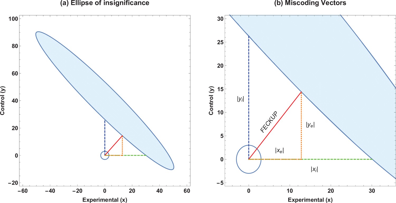
Ellipse of insignificance example.
(a) An example ellipse of insignificance for the , , , at a significance level of . All points bounded by the ellipse depict combinations which would not lead to the null being rejected. (b) Relevant vectors for ascertaining misconding thresholds. In this example, the Fewest Experimental/Control Knowingly Uncoded Participants (FECKUP) point is , , and . See text for details.
If we instead only consider inaccuracies in the experimental group as possible, we may set and for the equation of the ellipse, yielding the quadratic identity , readily solvable to determine xi. This is the point nearest the origin where the ellipse intercepts the x-axis. Conversely, we may consider a situation where only inaccuracies in the control group may exist. By similar reasoning, considering only inaccuracies in the control group yields a similar quadratic, to yield yi, the intercept of the ellipse with the y-axis. All these vectors are illustrated in Figure 1b, and are the maximum limits of miscoding theoretically possible before significance is lost.
Metrics for fragility of results
To ascertain if a trial or study is robust against the miscoding of patients or subjects, we introduce metrics to quantify this. Considering only inaccuracies in the experimental group, we define the tolerance threshold for error in experimental group as the fraction of subjects that must be correctly allocated in the experimental group to maintain significance, given by
This identity is intimately related to the existent FI, yielding the traditional FQ. For example, an experiment with after EOI analysis would inform us that up to 10% of experimental participants could be miscoded before the result lost significance. By similar reasoning, the tolerance threshold for error allowable in the control group is then
Finally, errors in both the coding of the experimental and control groups can be combined with FECKUP point knowledge. While gives a minimum vector distance to the ellipse, we instead take the length of the vector components to reflect to yield an absolute accuracy threshold of
Relating test sensitivity and specificity to miscoding thresholds
The identities derived thus far give a measure of the absolute accuracy required for confidence in the robustness of stated results. If details of the specific tests employed to determine endpoints in the experimental and control cohorts are known, then robustness can be directly related to the sensitivity and specificity of the tests employed. If the sensitivity () and specificity () of the test used to ascertain cases in the experimental group are known, then the observed number of cases with endpoint positive is related to the true number of endpoint positive cases, ao, by . It follows that the minimum miscoded cases in the experimental group are given by
A similar relationship can be derived for the control groups, with sensitivity and specificity , and the minimum miscoded cases in the control group are given by
The values denote the minimum miscoding that exists in reported figures because of inherent test limitations, and it follows that if this pair value lies within the EOI, then any ostensible results of the study are not robust. The forms given in Equations 15 and 16 are general forms. In many cases, when the same test is used in endpoint determination in the experimental and control groups, and . However, there are instances when in observational and cohort trials in particular, accrued data will derive from different tests on various cohorts, an example of which will be introduced later in this work.
Method inversion
It is important to note that the analysis presented here can be used not only to ascertain miscoding between endpoint positive and negative situations, but also can be inverted for situations where, for example, endpoint positive or negative might be known with high certainty but there are concerns over miscoding between control and experimental groups. In this case, simply reassigning endpoint positive, experimental and control groups, respectively, as () and endpoint negative experimental and control groups as () allows straightforward application of EOI analysis as outlined.
Polygon of insignificance
The EOI yields a continuously valued boundary. As only integer values are generally of concern, we can also define an irregular polygon of insignificance by considering the largest integer-valued polygon encompassing the EOI. Similarly, we can also take the floor values of , and yi in such an approach. This is readily derived from EOI analysis, and code to produce such a shape is included in the supplementary material.
Results
Illustrative example 1 – EOI analysis of published data
A previously published study claimed higher rates of miscarriage in a cohort with high magnetic field exposure () versus a low exposure cohort (), significant at . An EOI analysis shows that a displacement of less than two subjects would be enough to undo this seeming significance as shown in Figure 2, and that the absolute tolerance threshold was only as given in Table 2. This rendered the actual result highly fragile, given the demonstrable fact that inspection of the supplied tables in the paper in question demonstrated that at least nine subjects had been miscoded in the initial analysis. These weaknesses, coupled with the lack of a plausible biophysical hypothesis and non-physical dose–response curve, suggests such findings were likely spurious (Grimes and Heathers, 2021a).
Ellipse of insignificance (EOI) derived metrics for published data.
EOI statistic () | Derived value |
---|---|
Experimental group tolerance xi | 6.9 subjects |
Control group tolerance yi | 1.9 subjects |
FECKUP vector length | 1.9 subjects |
Tolerance threshold for error (experimental group) | 0.99% |
Tolerance threshold for error (control group) | 0.89% |
Absolute tolerance threshold for error (all subjects) | 0.22% |

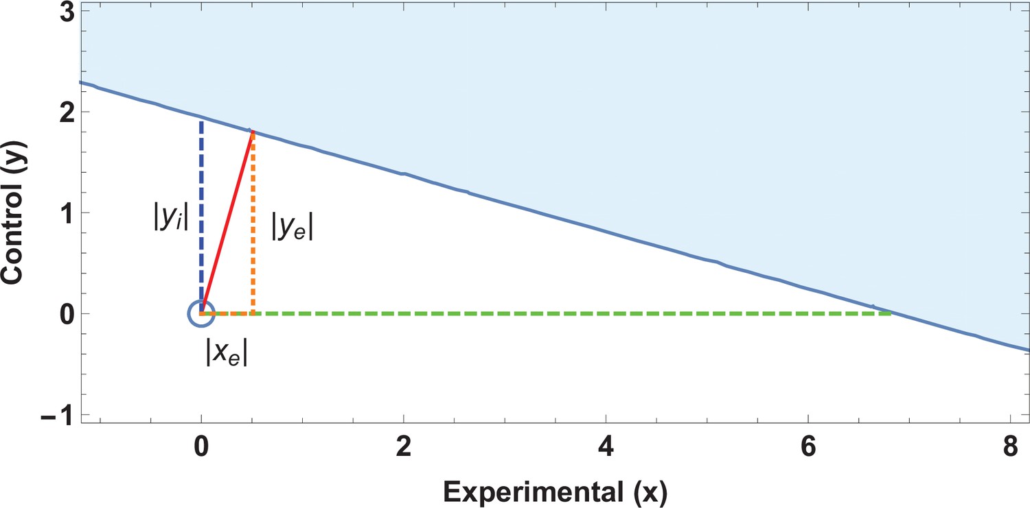
Application of ellipse of insignificance analysis to existent data.
(a) Ellipses of insignificance analysis for a published study (n = 913) for illustrative example 1 of published data. The shaded region denotes the ellipse of insignificance, the red line shows the Fewest Experimental/Control Knowingly Uncoded Participants (FECKUP) vector (the minimum vector from the origin to the ellipse).
Illustrative example 2 – EOI robustness analysis of similar results
Consider two hypothetical experiments that yield highly similar statistics. Experiment 1 has and Experiment 2 gives , both of which correspond to , and p values <0.00001. We can employ EOI analysis to ascertain how robust these seemingly strong respective results are for different values of . The EOI analysis and FECKUP vectors are illustrated in Figure 3 for , and relevant statistics for various values of are given in Table 3. It can be seen from this that despite the similar test statistics, Experiment 1 is consistently more robust, and would require the miscoding of at least 178 participants (8.9% of the entire sample) to lose significance, relative to 99 ( of the entire sample) in Experiment 2 at , a trend that continues even with lower values of .
Experimental metrics for similar test statistics.
Significance level | Data | |||
---|---|---|---|---|
Experiment 1 | 17.7% | 18.2% | 8.9% | |
Experiment 2 | 11% | 9.5% | 5.0% | |
Experiment 1 | 16.3% | 17.0% | 8.3% | |
Experiment 2 | 10.4% | 8.6% | 4.6% | |
Experiment 1 | 14.8% | 15.5% | 7.5% | |
Experiment 2 | 9.8% | 7.6% | 4.1% | |
Experiment 1 | 13.5% | 14.3% | 6.9% | |
Experiment 2 | 9.2% | 6.8% | 3.8% |

Illustrative example 2.
(a) Ellipses of insignificance analysis for two studies with same statistic. (b) Fewest Experimental/Control Knowingly Uncoded Participants (FECKUP) vectors for both studies. Experiment 1 is given by orange ellipse and red dotted line, Experiment 2 by the blue ellipse and dotted line.
Illustrative example 3 – sensitivity and specificity in cancer screening statistics
Consider an application of EOI analysis where sensitivity and specificity of different tests are being implicitly compared. Screening results derived from two hypothetical cities are listed in Table 4. City A uses standard Liquid-based cytology (LBC) analysis whereas City B’s programme uses a HPV(human papillomavirus)reflex scheme, where subjects are first tested for high-risk HPV. With , it would seem highly significant that these two cities have markedly different rates of CIN2+. The EOI analysis reveals that FECKUP vector details, as shown in Figure 4. Yet as the sensitivity and specificity of the respective tests are known (LBC: , , HPV-reflex: , ) application of Equation 14 yields . This exceeds xi and lies within the EOI, meaning we can immediately discount the ostensibly highly significant result despite its seeming strength. Further application of EOI analysis informed by sensitivity and specificity allows us to ascertain that the two cities actually have the same prevalence of CIN2, at 20 cases per 1000, a real problem encountered when comparing national screening programmes (Grimes et al., 2021c).

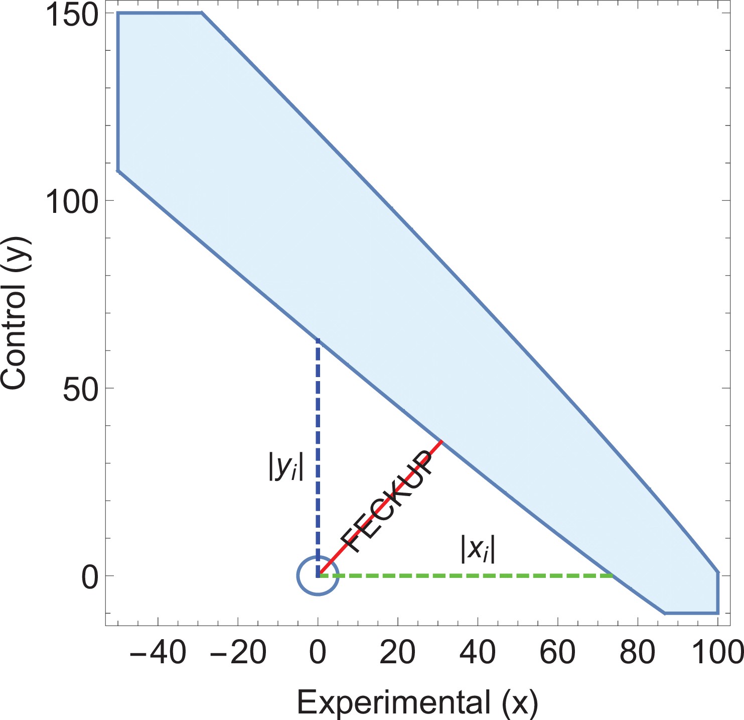
Illustrative example 3.
An ellipse of insignificance (EOI) analysis on the data supplied in the City A/City B screening comparison yields a Fewest Experimental/Control Knowingly Uncoded Participants (FECKUP) vector (in red) of 46.2 subjects, corresponding to a minimum tolerance of 66.5 total subjects after resolving the vector.
As (shown in green) with (shown in blue), but as the sensitivity and specificity of the tests used in City A are known, it can be shown that , exceeding the limits of xi, placing the point within the ellipse and rendering any seeming significance void. Note that only a part of the EOI (denoted by the blue solid shape) is shown for clarity.
Results of different analysis.
CIN2 + positive | No CIN2 + detected | Methodology | |
---|---|---|---|
City A (measured) | 113 | 887 | LBC only |
City B (measured) | 24 | 976 | HPV screening/LBC reflex |
True values (both cities) | 20 | 980 | N/A |
Discussion
The analysis presented here is a deterministic way to ascertain the fragility of a given dichotomous outcome study by considering experimental and control groups in concert. This method is geometrical in origin and computationally inexpensive. It also explicitly can relate outcome fragility to the sensitivity and specificity of tests employed when known, aiding clinicians and meta-researchers in interpreting the trustworthiness of a given study. Sample OCTAVE and MATLAB code and stand-alone Windows applications are provided to run the analysis outlined in this work, available in the electronic supplementary material. There are a number of limitations of this work that should be explicitly discussed, and caveats to be elucidated. The EOI analysis handles potential miscoding, but cannot be used to infer anything about patients or subjects lost to follow-up. This is a weakness of all FI/FQ methods, as it is not a priori knowable from reported data alone why patients dropped out, or why they might have atrophied from particular subgroups. Redaction bias (Grimes and Heathers, 2021b) can occur if subjects leave a particular subset at an elevated rate, and while beyond the scope of this work, it is important to realize that explicit connections between EOI/FI/FQ analysis and numbers lost to follow-up cannot be directly made. The method outlined is deterministic and rapid, but only currently applicable to dichotomous outcome trials and studies, and should be applied very cautiously to time-to-event data, where it may not be suitable. FI itself is also typically calculated using Fisher’s exact test, which well approximates a chi-squared test. However, for small trials, the p value derived from Fisher’s exact test can be discrepant from chi-squared result. When Fisher’s exact test produces a non-significant p value without any recoding, an FI of 0 results, suggesting a distinct lack of robustness of the underlying data. As EOI analysis is built upon chi-squared statistics, it is possible in edge cases of small numbers to have discordant results between EOI and Fisher’s exact test also. The chief advantage of the method outlined here, however, is that it handles extremely large data sets with ease. In large data sets, Fischer’s exact test breaks down due to its dependence on factorials, and a chi-squared approximation is more appropriate. This is fitting, given EOI is built upon the chi-square distribution. But the important caveat is that for rare events in small trials, an FI approach built upon Fisher’s exact test may be more appropriate (Baer et al., 2021a). The usage of FI/FQ itself remains contested in the literature, and one frequent objection is that the mere existence of a small FI might be an artefact of trial design (Walter et al., 2020). With clinical RCTs in particular, experimenters often design trials to minimize exposure of patients or subjects to as of yet unknown harms, while seeking to ensure enough of them participate so that clinically relevant causal effects can be reliably detected. From this vantage point, RCTs might be fragile ‘by design’. This view is countered by other authors Baer et al., 2021a who argue that there are no evidence p value distributions tend to cluster around the significance threshold after a sample size calculation, and that the FI in well-designed studies is not always low (Baer et al., 2021b). This work does not comment on the absolute applicability of the FI, but offers new metrics for quantification of results in context. More importantly, EOI analysis has definite application for dichotomous outcome results not derived just from fragile-by-design RCTs, but from ecological studies, cohort trials, and preclinical work which should in principle be far more resilient to investigation than RCTs. There is a less edifying but important reason why EOI analysis might be conducted – the detection of questionable research practices and fraud. While most scientists and clinicians operate ethically, poor conduct and inappropriate statistical manipulation can and do occur. By some estimates, up to three quarters of all biomedical science are affected by poor practice (Fanelli, 2009), casting doubt on results to the detriment of science and the public, often a consequence of publish-or-perish pressure (Grimes et al., 2018). During the COVID-19 pandemic, a number of dubious high-profile results have come to light, particularly on drugs like Ivermectin (Hill et al., 2022; Besançon et al., 2022). EOI analysis has a potential role in detecting manipulations that nudge results towards significance, and identifying inconsistencies in data. EOI analysis is perhaps ideal for this purpose, as it explicitly relates known test sensitivity and specificity to projected error tolerance, allowing detection of suspect results in even large data sets, as illustrated by the real examples in this work. Despite its caveats on usage, the FI has seen growing application in analysis of trial outcomes, and the EOI system presented here should allow this to be applied more thoroughly in a multidimensional way. Regardless of whether appropriate research practice has been observed or not, it is important to be able to estimate the soundness of results in biomedical science, to ascertain what level of confidence once can ascribe to them. This need has seen the recent resurgence of FI analysis, and the EOI analysis presented here can help undercover questionable results and experimental inconsistencies, with wide potential application in meta-research and reproducible research.
Data availability
The paper is a modelling study and methodology and contains no data, and code provided in the supplementary material allows reproduction of all methods.
References
-
Points of significance: Interpreting P valuesNature Methods 14:213–215.https://doi.org/10.1038/nmeth.4210
-
The fragility index can be used for sample size calculations in clinical trialsJournal of Clinical Epidemiology 139:199–209.https://doi.org/10.1016/j.jclinepi.2021.08.010
-
A critique of the fragility indexThe Lancet. Oncology 20:e551.https://doi.org/10.1016/S1470-2045(19)30582-0
-
An investigation of the false discovery rate and the misinterpretation of p-valuesRoyal Society Open Science 1:140216.https://doi.org/10.1098/rsos.140216
-
A critique of the fragility index-authors ’ replyThe Lancet. Oncology 20:e554.https://doi.org/10.1016/S1470-2045(19)30580-7
-
A critique of the fragility indexThe Lancet. Oncology 20:e552.https://doi.org/10.1016/S1470-2045(19)30583-2
-
The unit fragility index: an additional appraisal of “ statistical significance ” for a contrast of two proportionsJournal of Clinical Epidemiology 43:201–209.https://doi.org/10.1016/0895-4356(90)90186-s
-
Modelling science trustworthiness under publish or perish pressureRoyal Society Open Science 5:171511.https://doi.org/10.1098/rsos.171511
-
Oxygen diffusion in ellipsoidal tumour spheroidsJournal of the Royal Society, Interface 15:20180256.https://doi.org/10.1098/rsif.2018.0256
-
The new normal? redaction bias in biomedical scienceRoyal Society Open Science 8:211308.https://doi.org/10.1098/rsos.211308
-
The fickle P value generates irreproducible resultsNature Methods 12:179–185.https://doi.org/10.1038/nmeth.3288
-
Ivermectin for covid-19: addressing potential bias and medical fraudOpen Forum Infectious Diseases 9:ofab645.https://doi.org/10.1093/ofid/ofab645
-
A critique of the fragility indexThe Lancet. Oncology 20:e553.https://doi.org/10.1016/S1470-2045(19)30581-9
-
The fragility index in multicenter randomized controlled critical care trialsCritical Care Medicine 44:1278–1284.https://doi.org/10.1097/CCM.0000000000001670
-
The statistical significance of randomized controlled trial results is frequently fragile: a case for a fragility indexJournal of Clinical Epidemiology 67:622–628.https://doi.org/10.1016/j.jclinepi.2013.10.019
-
The fragility of trial results involves more than statistical significance aloneJournal of Clinical Epidemiology 124:34–41.https://doi.org/10.1016/j.jclinepi.2020.02.011
Decision letter
-
Philip BoonstraReviewing Editor; University of Michigan, United States
-
Mone ZaidiSenior Editor; Icahn School of Medicine at Mount Sinai, United States
-
Philip BoonstraReviewer; University of Michigan, United States
-
Fei JiangReviewer; UCSF, United States
In the interests of transparency, eLife publishes the most substantive revision requests and the accompanying author responses.
Decision letter after peer review:
[Editors’ note: the authors submitted for reconsideration following the decision after peer review. What follows is the decision letter after the first round of review.]
Thank you for submitting the paper "The Ellipse of Insignificance: a refined fragility index for ascertaining robustness of results in dichotomous outcome trials" for consideration by eLife. My apologies for the delay in getting these reviews returned to you. Your article has been reviewed by 2 peer reviewers, including Philip Boonstra as the Reviewing Editor and Reviewer #1, and the evaluation has been overseen by a Senior Editor. The following individual involved in review of your submission has agreed to reveal their identity: Fei Jiang (Reviewer #2).
Comments to the Authors:
We are sorry to say that, after consultation with the reviewers, we have decided that this work will not be considered further for publication by eLife.
Specifically, as the reviewers note, the proposed approach does not adequately address the limitations of the existing family of fragility indices and therefore seems to suffer from the same limitations as the methods it is intended to improve upon, and the improvement over the fragility index is neither characterized or quantified.
Reviewer #1 (Recommendations for the authors):
This article extends the concept of the fragility index for clinical trials using geometric arguments. The proposed approach is a two-step calculation. First, the two-dimensional ellipsis that contains the insignificance region is calculated, where each dimension represents one of the two arms in the trial. Then, the shortest vector between the trial's actual result and this ellipsis is identified. Shorter-length vectors point to greater fragility in the findings.
The idea of the fragility index is to measure how many subjects' outcomes would need to be changed in order to change the qualitative conclusion of a trial. The author raises several challenges to the fragility index: a lack of feasibility for time-to-event outcomes, a lack of clear distinction between 'robust' versus 'fragile', the need to calculate Fisher's exact test multiple times, and, in some cases, an inability to deal with fragility in both treatment arms at the same time.
Unfortunately, the proposed idea, although mathematically very intriguing, does not ultimately address these stated deficiencies, which limits its utility. Specifically, there is no solution proposed for the issue of time-to-event outcomes; there is no resolution to the issue of distinguishing between robust and fragile; and the perceived computational burden of calculating multiple Fisher's exact tests is actually not particularly great given the computational power of today's personal computers. Thus, the primary contribution of this article – from this reviewer's perspective – is with regard to the ability to generalize the fragility index to considering changes in both arms simultaneously.
Separately – I wonder if it would be more appropriate to define an irregular polygon of insignificance, defined as the largest polygon that is encompassed by the EOI and is comprised of connected segments of integer valued (x,y) coordinates. My thinking here is that since it is impossible to have continuously valued counts of responses, one should only consider integer-valued (x,y) coordinates as possibilities.
It may also be worthwhile to compare and contrast the difference in assumptions and approximations between Fisher's exact test and a chi-squared analysis.
1. The chosen acronym (FECKUP) is very similar-sounding and similar-looking to an English-language vulgarity. I wonder if the author might consider a different choice of acronym for their index.
2. The definitions of Qe, Qc, and Qa in Inequalities (11), (12), and (13), respectively, are somewhat unclear. Since these are inequalities, the mathematical implication is that Qe, Qc, and Qa can be any values less than their upper bounds, as in rows 4 and 5 of Table, whereas they are presented as single values in Table 3. I think the intent is to define Qe, Qc, and Qa as being equal to these upper bounds and to then claim that these are 'best case' scenarios for these different error types. Can the author please clarify/change how precisely to interpret Qe, Qc, and Qa and potentially consider changing these expressions in the manuscript?
Reviewer #2 (Recommendations for the authors):
This paper provides a potentially useful tool for conducting reproducible research with binary endpoints. The work provides steps to construct evaluation criteria of how sensitive a scientific conclusion regarding the changes of the observations. Overall, the study problem is important, but the proposed methods are not fully evaluated against the existing approach to justify the superiority of the method.
Strengths:
The derivation of the measurement is comprehensive.
Two case studies are interesting
Weaknesses:
No comparison with the existing method.
The author claim that the method is computationally inexpensive, but did not report the computational time for the proposed method and the existing method.
It is not clear what the improvement the proposed method made upon the existing method.
Impact:
The new tool can be useful for conducting reproducible research if the methods have been validated more rigorously.
Suggestions:
1, The paper will benefit from adding some simulation studies to justify the superiority of the method.
2, The author should be more precise about their terminologies. For example, what does "minimal error", "maximal proportion error" refer to? Also (11), (12), and (13) only provide upper bound of Qe, Qc, Qa, not their exact values. It is not clear why Qa reported in Table 2 has an exact solution. Please clarify.
3, The authors must compare with existing methods in real data examples.
[Editors’ note: further revisions were suggested prior to acceptance, as described below.]
Thank you for resubmitting your work entitled "The Ellipse of Insignificance, a refined fragility index for ascertaining robustness of results in dichotomous outcome trials" for further consideration by eLife. Your revised article has been evaluated by Mone Zaidi (Senior Editor) and a Reviewing Editor. Thanks also for your patience in getting this review back to you.
The manuscript has been improved but there are some remaining issues that need to be addressed, as outlined below.
Reviewer #1 (Recommendations for the authors):
Thanks to the author for their revised submission. Now that I have a better understanding of the approach, I do unfortunately have some additional questions, not all of which were raised in my initial review.
1. I am confused by the difference in definition between x_i vs x_m and y_i vs y_m. The legend in Figure 2 states that the green line depicts x_i, whereas the caption in Figure 2 caption states that the green line depicts x_m. Similarly, Table 1 also implies that x_m is the green line by virtue of stating that it is equal to 6.9. In fact, x_i is not explicitly defined in the manuscript as far as I can tell, but based upon the paragraph before equation (11), I believe it is interpreted as 'the number of subjects in the experimental group with a recorded positive endpoint who would need to be reclassified to negative in order for the study to lose statistical significance at the given significance threshold, holding fixed all measurements in the control group'. And y_i would be defined analogously. I think these are more or less the classic FI metrics. And therefore, I believe that the green line in Figure 2 is x_i, not x_m. In contrast, x_m and y_m must take into account some external knowledge/assumptions about the sensitivity and specificity of the measurement process; these values cannot be learned from the data itself. The sentence just before equations (14) and (15) states that x_m and y_m are the 'minimum miscoded cases', but I believe they are more appropriately defined as an 'anticipated number of miscoded cases given presumed values of specificity and sensitivity' (in particular, I would argue that they should be written as functions of se and sp: xm(se, sp)). If my understanding about this is all correct, I do not believe these definitions are adequately communicated in the manuscript and sometimes contradictorily used (e.g. in the caption of Figure 2). I would suggest, for example, that in the illustrative example on the bottom of page 4, it is clearly stated what x_i and y_i are, what the presumed values of se and sp are, and therefore what the presumed values of x_m and y_m are (as a related aside: how is the reader supposed to know that it is demonstrable fact that at least 9 patients had been miscoded? Is this discussed in the reference?).
2. Thanks to the author for clarifying the definitions of Qe, Qc, and Qa (now defined as epsilon_E, etc). I especially appreciate the added sentence between equations (11) and (12) that interpret it for a non-statistical audience. However, I see that the Methods section has been moved after the Results and Discussion section. I am not strictly opposed to this decision; however, the result is that readers who read through the manuscript as it is written will see these novel technical terms used prior to their definitions. I suggest that the author either return to the ordering of sections that is more traditionally used for statistical articles and which was used in the original submission (Introduction, Methods, Results, Discussion) or add references to defining equations for any novel technical terms used at their first use and a simple, non-statistical interpretation.
3. If the definitions /distinctions between x_i and x_m can be cleared up as per my first comment above, are the epsilons really necessary at all? Put differently, can the author please clarify why these statistics offer distinct information? Epsilon_A would seem to be just a rescaling of x_i by the sample size.
4. Figure 4: I suggest to add a parenthetical that the FECKUP vector is in red. A legend such as what is used in Figure 2 would be helpful.
5. Also, in the spirit of creating Figures that 'stand alone', can the caption of Figure 4 be modified to make clear which illustrative example it refers to? The only evidence that Figure 4 refers to the hypothetical liquid biopsy data is the use of the term 'city A' in the second sentence of the caption.
6. Figure 2 is not referenced anywhere in the text of the manuscript (as far as I can tell).
7. Can the author please add some sort of enumerative label or title to each of the illustrative examples and ensure that tables and figures make clear in their captions which illustrative example they refer to?
8. The third paragraph of the discussion says the method is 'only currently applicable to dichotomous outcome trials' but, assuming that the word 'trial' refers to an active intervention, I believe the author intends that this approach is more widely applicable to any study (that is, both interventional and observational) with a non-censored dichotomous endpoint.
9. I am still unclear on the need for the inequality in (13): does this inequality give a definition of epsilon_a, i.e. is epsilon_a really the entire set of numbers less than the RHS of this inequality? If so, why is epsilon_a only ever given as a single number and not an interval?
10. Figure 4: presuming this Figure refers to the cancer screening example, the units of analysis here are more appropriately referred to as 'subjects' not 'patients'. This comment applies more broadly, i.e. the second paragraph of the discussion.
11. The statement immediately following (15): "If xm >= xi or ym >= yi or both conditions are met…". Should there be absolute values around these expressions? For example, if xi < 0 and xm=0, then the sentence as currently written suggests that the results are not robust, which seems misleading. I believe the intended meaning here is "If |xm| >= |xi| or |ym| >= |yi| or both conditions are met…".
https://doi.org/10.7554/eLife.79573.sa1Author response
[Editors’ note: The authors appealed the original decision. What follows is the authors’ response to the first round of review.]
Reviewer #1 (Recommendations for the authors):
This article extends the concept of the fragility index for clinical trials using geometric arguments. The proposed approach is a two-step calculation. First, the two-dimensional ellipsis that contains the insignificance region is calculated, where each dimension represents one of the two arms in the trial. Then, the shortest vector between the trial's actual result and this ellipsis is identified. Shorter-length vectors point to greater fragility in the findings.
The idea of the fragility index is to measure how many subjects' outcomes would need to be changed in order to change the qualitative conclusion of a trial. The author raises several challenges to the fragility index: a lack of feasibility for time-to-event outcomes, a lack of clear distinction between 'robust' versus 'fragile', the need to calculate Fisher's exact test multiple times, and, in some cases, an inability to deal with fragility in both treatment arms at the same time.
1. Unfortunately, the proposed idea, although mathematically very intriguing, does not ultimately address these stated deficiencies, which limits its utility. Specifically, there is no solution proposed for the issue of time-to-event outcomes; there is no resolution to the issue of distinguishing between robust and fragile; and the perceived computational burden of calculating multiple Fisher's exact tests is actually not particularly great given the computational power of today's personal computers. Thus, the primary contribution of this article – from this reviewer's perspective – is with regard to the ability to generalize the fragility index to considering changes in both arms simultaneously.
This is a very helpful comment and raises important aspects I’ll address here. Firstly, part of the problem is that I did not clarify the true motivation for this work: to not only consider relatively small RCTs but to create a robust framework for observational, longitudinal, cohort, and preclinical trials with dichotomous outcomes, tied directly to the properties of the statistical tests used to create that dictomization in the first instance. While this method doesn’t resolve time-to-event problem, it is capable of handling huge trials where Fischer’s exact test would struggle or fail due to its inherent reliance on factorials. This makes it rugged and capable of handling much more than RCTs. And more than this, because of the equations 14 and 15, we can in many cases directly contrast the explicit fragility with the theoretical thrust limits given by the tests involved, which will allow us to rule out many stated results without having to arbitrarily set a threshold, as discussed above. This makes it highly suitable for automated meta-analysis, and detection of fraud.
I have accordingly re-written the introduction and discussion text to reflect this motivation better, with the modified passages now reading:
“In this work, I introduce a geometric refinement of the concept underpinning FI which overcomes some difficulties associated with FI analysis, considering recoding in both control and experimental groups in tandem. This ellipse of insignificance (EOI) approach is exact and computationally inexpensive, yielding objective measures of experimental robustness. There are two major differences and situational advantages to such a formulation; firstly, it can handle huge data sets with ease and consider both control and experimental arms simultaneously, which traditional fragility analysis cannot. Previously, fragility has been typically considered in the case of relatively small numbers in Randomized controlled trials, which as previous commentators have noted are often fragile by design. The method outlined here handles massive numbers with ease, rendering it suitable for analysis of observational trials, cohort studies, and general preclinical work, to detect dubious results and fraud. This sets it apart in both intention and application to existing measures, and makes it unique in this regard.
Secondly, this methodology is not solely a new, robust fragility index; it also goes further by linking the concept of fragility to test sensitivity and specificity. This {a priori} allows an investigator to probe not only whether a result is arbitrarily fragile, but to truly probe whether consider certain results are even possible. This renders it less arbitrary than existent measures, as it ties directly statistically measurable quantities to stated results, and is sufficiently powerful to rule out suspect findings in many dichotomous trials. It can accordingly be used to detect likely fraud or inappropriate manipulation of results if the statistical properties of the tests used are known. This is unfortunately highly relevant, as unsound or otherwise manipulated results have become an increasingly recognised problem in biomedical research, and means to detect them are vital.”
2. Separately – I wonder if it would be more appropriate to define an irregular polygon of insignificance, defined as the largest polygon that is encompassed by the EOI and is comprised of connected segments of integer valued (x,y) coordinates. My thinking here is that since it is impossible to have continuously valued counts of responses, one should only consider integer-valued (x,y) coordinates as possibilities.
This is an excellent suggestion and echoes one made to me by readers of the preprint. I have already created a method for precisely doing this which compliments the existing ellipse method, and this is now incorporated into the manuscript and the sample code. The results are broadly similar to the EOI method, but it is a useful addition to consider. The new text reads:
“The ellipse of insignificance yields a continuously valued boundary. As only integer values are generally of concern, we can also define an irregular polygon of insignificance (POI) by considering the largest integer-valued polygon encompassing the EOI. Similarly, we can also take the floor values of xe, ye ,xi, and yi in such an approach. This is readily derived from EOI analysis, and code to produce such a shape is included in the supplementary material.”
3. It may also be worthwhile to compare and contrast the difference in assumptions and approximations between Fisher's exact test and a chi-squared analysis.
This is an excellent idea too to elucidate differences. As I have clarified now in reply point 1 about the application being different, it’s worth stressing the differences again for comparison. In the discussion, I’ve added the text:
“As EOI analysis is built upon chi squared statistics, it is possible in edge cases of small numbers to have discordant results between EOI and Fisher's exact test also. The chief advantage of the method outlined here, however, is that it handles extremely large data sets with ease. In large data sets, Fischer's exact test breaks down due to its dependence on factorials, and a chi-squared approximation is more appropriate. This is fitting, given EOI is built upon the chi-square distribution.
But the important caveat is that for rare events in small trials, a Fragility index approach built upon Fisher's exact test may be more appropriate.”
4. The chosen acronym (FECKUP) is very similar-sounding and similar-looking to an English-language vulgarity. I wonder if the author might consider a different choice of acronym for their index.
This is true and partly tongue-in-cheek; in Hiberno and British English ‘feck’ is a sanitised and more gentle version of the more common vulgarity, and I chose it here in part because the natural acronym that arose alluded to the idea of messing something up without the aggressive qualities of the more Germanic term. I am completely happy to change this if the reviewer and editors wish, and am happy to act on their advice and change or leave it as requested.
5. The definitions of Qe, Qc, and Qa in Inequalities (11), (12), and (13), respectively, are somewhat unclear. Since these are inequalities, the mathematical implication is that Qe, Qc, and Qa can be any values less than their upper bounds, as in rows 4 and 5 of Table, whereas they are presented as single values in Table 3. I think the intent is to define Qe, Qc, and Qa as being equal to these upper bounds and to then claim that these are 'best case' scenarios for these different error types. Can the author please clarify/change how precisely to interpret Qe, Qc, and Qa and potentially consider changing these expressions in the manuscript?
I think this is a very fair criticism that has been echoed by preprint comments, and it is apparent that my initial formulation lacked clarity. I have totally rewritten this section (and all related figures) and also altered the metrics slight to be more intuitive, and instead defined the quantities as tolerances. For example, I know define εE as the tolerance threshold for error in the experimental group; for example, if εE = 0.1, that is the same as observing that 10% of the control group could be recoded from event to non-event (or vice versa) before seeming significant was lost. This tolerance is more intuitive, and I’ve changed the metric throughout: see ‘Metrics for fragility of results’:
Reviewer #2 (Recommendations for the authors):
1. This paper provides a potentially useful tool for conducting reproducible research with binary endpoints. The work provides steps to construct evaluation criteria of how sensitive a scientific conclusion regarding the changes of the observations. Overall, the study problem is important, but the proposed methods are not fully evaluated against the existing approach to justify the superiority of the method.
The major strength of this method lies in ruggedness of the method to huge trials (not just RCTs) and its ability to relate results to the sensitivity / specificity of the actual tests used to dictomize the data. It is accordingly useful for fraud detection, and for identifying weak results without the same arbitrariness of other metrics in many cases. Please see replies 1 and 3 to reviewer 1.
Suggestions:
1, The paper will benefit from adding some simulation studies to justify the superiority of the method.
2, The author should be more precise about their terminologies. For example, what does "minimal error", "maximal proportion error" refer to? Also (11), (12), and (13) only provide upper bound of Qe, Qc, Qa, not their exact values. It is not clear why Qa reported in Table 2 has an exact solution. Please clarify.
This is absolutely true, and resonates with comments by reviewer 1 point 5. I have made these much more solid and intuitive in the current iteration, and please see reply to reviewer 1 point 5 for specific details.
[Editors’ note: what follows is the authors’ response to the second round of review.]
The manuscript has been improved but there are some remaining issues that need to be addressed, as outlined below.
Reviewer #1 (Recommendations for the authors):
Thanks to the author for their revised submission. Now that I have a better understanding of the approach, I do unfortunately have some additional questions, not all of which were raised in my initial review.
1. I am confused by the difference in definition between x_i vs x_m and y_i vs y_m. The legend in Figure 2 states that the green line depicts x_i, whereas the caption in Figure 2 caption states that the green line depicts x_m. Similarly, Table 1 also implies that x_m is the green line by virtue of stating that it is equal to 6.9. In fact, x_i is not explicitly defined in the manuscript as far as I can tell, but based upon the paragraph before equation (11), I believe it is interpreted as 'the number of subjects in the experimental group with a recorded positive endpoint who would need to be reclassified to negative in order for the study to lose statistical significance at the given significance threshold, holding fixed all measurements in the control group'. And y_i would be defined analogously. I think these are more or less the classic FI metrics. And therefore, I believe that the green line in Figure 2 is x_i, not x_m. In contrast, x_m and y_m must take into account some external knowledge/assumptions about the sensitivity and specificity of the measurement process; these values cannot be learned from the data itself. The sentence just before equations (14) and (15) states that x_m and y_m are the 'minimum miscoded cases', but I believe they are more appropriately defined as an 'anticipated number of miscoded cases given presumed values of specificity and sensitivity' (in particular, I would argue that they should be written as functions of se and sp: xm(se, sp)). If my understanding about this is all correct, I do not believe these definitions are adequately communicated in the manuscript and sometimes contradictorily used (e.g. in the caption of Figure 2). I would suggest, for example, that in the illustrative example on the bottom of page 4, it is clearly stated what x_i and y_i are, what the presumed values of se and sp are, and therefore what the presumed values of x_m and y_m are (as a related aside: how is the reader supposed to know that it is demonstrable fact that at least 9 patients had been miscoded? Is this discussed in the reference?).
I thank the reviewer for raising this, as it lays bare how clumsy I had been with my terminology, partially a consequence of multiple iterations getting confused. I have amended the text and images very substantially in this revision. Briefly, if we consider the ellipse of insignificance, the FECKUP vector is the closest line from the origin to this ellipse. The resolution of this vector gives us (xm, ym), the absolute minimum number of experimental and control subjects respectively would have to be miscoded for significance to vanish. The value (xi) arises from a hypothetical situation where only experimental subjects can vary (we have perfect accuracy in control subjects), which corresponds to the ellipse intersecting the x-axis. Conversely, we have (yi), the hypothetical situation where the experimental arm is perfectly accurate, but the control arm can vary. This is where the ellipse intersects the y-axis. In the new 2-part figure 1, I have now hopefully made this much clearer. These points allow us to state the maximum tolerance for miscoding we can even hypothetically have, bounded between the two extremes. I hope that the new figure 1(b) remedies this somewhat.
The situation for (xm,ym) was also poorly elucidated by me originally – my apologies, I was very unclear in my phrasing. Put simply, if a test for sorting between events and non-events is not perfect but has some known sensitivity and specificity, then it follows that the reported numbers will be affected by this. The identities established in this work allow us to work backwards, and explicitly determine how many cases must be miscoded for a known test sensitivity / specificity. We can then derive this pair from the equations outlined, and check whether (xm, ym) lies within the ellipse of insignificance. If it does, as in the cancer screening example, we can confidently state that any seeming significance is entirely illusory. I was clumsy in this phrasing and contradictory, and have now rewritten these sections for clarity. It was confusing to relate these to (xi) because, more intuitively, all we need to do so show a result is not robust is show (xm,ym) lies within the ellipse of insignificance. I have rewritten the section now to account for this, explicitly stating
“The values for (xm, ym) denote the minimum miscoding that exists in reported figures because of inherent test limitations, and it follows that if this pair-value lies within the ellipse of insignificance, then any ostensible results of the study are not robust.”
Hopefully this clarifies somewhat – in relation to the figures, the reviewer is absolutely correct that there were contradictions in the captions and graphics. This was remiss of me, my apologies again. To correct this, I have reproduced figure 2 with the vector lengths explicitly shown and caption redone. This is shown overleaf in context.
The reviewer also correctly noted that I mention 9 subjects miscoded without specifying where this came from. It is indeed buried in the reference, but its introduction without explicitly saying this was jarring – I have now rephrased the section to read:
“This rendered the actual result highly fragile, given the demonstrable fact that inspection of the supplied tables in the paper in question demonstrated that at least 9 patients had been miscoded in the initial analysis.”
2. Thanks to the author for clarifying the definitions of Qe, Qc, and Qa (now defined as epsilon_E, etc). I especially appreciate the added sentence between equations (11) and (12) that interpret it for a non-statistical audience. However, I see that the Methods section has been moved after the Results and Discussion section. I am not strictly opposed to this decision; however, the result is that readers who read through the manuscript as it is written will see these novel technical terms used prior to their definitions. I suggest that the author either return to the ordering of sections that is more traditionally used for statistical articles and which was used in the original submission (Introduction, Methods, Results, Discussion) or add references to defining equations for any novel technical terms used at their first use and a simple, non-statistical interpretation.
I thank the reviewer for this observation, and agree it would be much easier to follow the flow if the typical ordering for such papers is allowed rather than putting the methodology at the end. I have redone the paper this way now. If ELife allow this, I agree it reads better – if not, I will tyr to re-write so that terms are defined in context. I am happy to chat with editorial team on this.
3. If the definitions /distinctions between x_i and x_m can be cleared up as per my first comment above, are the epsilons really necessary at all? Put differently, can the author please clarify why these statistics offer distinct information? Epsilon_A would seem to be just a rescaling of x_i by the sample size.
Hopefully my reply to point 1 and subsequent rewrite has clarified matters somewhat – my poor phrasing wrongly created a link between xm and xi which is hopefully clarified in this iteration.
4. Figure 4: I suggest to add a parenthetical that the FECKUP vector is in red. A legend such as what is used in Figure 2 would be helpful.
I whole-heartedly agree – figure has been re-rendered, and caption text modified as per points 5, 7 and 10.
5. Also, in the spirit of creating Figures that 'stand alone', can the caption of Figure 4 be modified to make clear which illustrative example it refers to? The only evidence that Figure 4 refers to the hypothetical liquid biopsy data is the use of the term 'city A' in the second sentence of the caption.
This is a very useful point, and I have modified all captions in light of this observation and the points raised in 7 and 10 after this. The new figure 4 caption text reads:
“Illustrative example 3 – An EOI analysis on the data supplied in the City A / City B screening comparison yields a FECKUP vector (in red) of 46.2 subjects, corresponding to a minimum tolerance of 66.5 total subjects after resolving the vector. As xi = 73.7 (shown in green) with yi = 62.7$ (shown in blue), but as the sensitivity and specificity of the tests used in city A are known, it can be shown that xm ≈ 93, exceeding the limits of xi, placing the point within the ellipse and rendering any seeming significance void. Note that only a part of the ellipse of insignificance (denoted by the blue solid shape) is shown for clarity”
6. Figure 2 is not referenced anywhere in the text of the manuscript (as far as I can tell).
This is true, and is remedied now, thank you.
7. Can the author please add some sort of enumerative label or title to each of the illustrative examples and ensure that tables and figures make clear in their captions which illustrative example they refer to?
This has now been done for all figures and examples.
8. The third paragraph of the discussion says the method is 'only currently applicable to dichotomous outcome trials' but, assuming that the word 'trial' refers to an active intervention, I believe the author intends that this approach is more widely applicable to any study (that is, both interventional and observational) with a non-censored dichotomous endpoint.
This is absolutely true, and I have rewritten the discussion and introduction section to append the studies aspect, as I see this method having wider application in cohort studies and preclinical work.
9. I am still unclear on the need for the inequality in (13): does this inequality give a definition of epsilon_a, i.e. is epsilon_a really the entire set of numbers less than the RHS of this inequality? If so, why is epsilon_a only ever given as a single number and not an interval?
My apologies again, this was an artifact from a prior version – the equality is now there as it should have been previously.
10. Figure 4: presuming this Figure refers to the cancer screening example, the units of analysis here are more appropriately referred to as 'subjects' not 'patients'. This comment applies more broadly, i.e. the second paragraph of the discussion.
This is a very pertinent point – I have now corrected the manuscript to take this onboard in multiple areas.
11. The statement immediately following (15): "If xm >= xi or ym >= yi or both conditions are met…". Should there be absolute values around these expressions? For example, if xi < 0 and xm=0, then the sentence as currently written suggests that the results are not robust, which seems misleading. I believe the intended meaning here is "If |xm| >= |xi| or |ym| >= |yi| or both conditions are met…".
The reviewer is absolutely correct to note this – hopefully I have made it clearer that the only criteria that matter is as outlined in point 1 and 3, namely that the point (xm,ym) lies within the ellipse of insignificance.
https://doi.org/10.7554/eLife.79573.sa2Article and author information
Author details
Funding
Wellcome Trust (214461/A/18/Z)
- David Robert Grimes
The funders had no role in study design, data collection, and interpretation, or the decision to submit the work for publication. For the purpose of Open Access, the authors have applied a CC BY public copyright license to any Author Accepted Manuscript version arising from this submission.
Acknowledgements
DRG thanks the Wellcome trust for their support, Dr Darren Dahly for insight into aspects of trial design, Dr Nick Brown for his proofing, and Dr James Heathers for encouragement, discussions, and creative profanity. He would also like to thank Dr Ben Baer, Dr Martin T Wells, and Faheem Gilani for their helpful comments on this manuscript. He could also like to extend this thanks to the reviewers for their diligence and advice.
Senior Editor
- Mone Zaidi, Icahn School of Medicine at Mount Sinai, United States
Reviewing Editor
- Philip Boonstra, University of Michigan, United States
Reviewers
- Philip Boonstra, University of Michigan, United States
- Fei Jiang, UCSF, United States
Version history
- Preprint posted: March 28, 2022 (view preprint)
- Received: April 19, 2022
- Accepted: September 13, 2022
- Accepted Manuscript published: September 20, 2022 (version 1)
- Version of Record published: October 21, 2022 (version 2)
Copyright
© 2022, Grimes
This article is distributed under the terms of the Creative Commons Attribution License, which permits unrestricted use and redistribution provided that the original author and source are credited.
Metrics
-
- 536
- Page views
-
- 85
- Downloads
-
- 0
- Citations
Article citation count generated by polling the highest count across the following sources: Crossref, PubMed Central, Scopus.
Download links
Downloads (link to download the article as PDF)
Open citations (links to open the citations from this article in various online reference manager services)
Cite this article (links to download the citations from this article in formats compatible with various reference manager tools)
Further reading
-
- Epidemiology and Global Health
- Genetics and Genomics
Accurate inference of who infected whom in an infectious disease outbreak is critical for the delivery of effective infection prevention and control. The increased resolution of pathogen whole-genome sequencing has significantly improved our ability to infer transmission events. Despite this, transmission inference often remains limited by the lack of genomic variation between the source case and infected contacts. Although within-host genetic diversity is common among a wide variety of pathogens, conventional whole-genome sequencing phylogenetic approaches exclusively use consensus sequences, which consider only the most prevalent nucleotide at each position and therefore fail to capture low frequency variation within samples. We hypothesized that including within-sample variation in a phylogenetic model would help to identify who infected whom in instances in which this was previously impossible. Using whole-genome sequences from SARS-CoV-2 multi-institutional outbreaks as an example, we show how within-sample diversity is partially maintained among repeated serial samples from the same host, it can transmitted between those cases with known epidemiological links, and how this improves phylogenetic inference and our understanding of who infected whom. Our technique is applicable to other infectious diseases and has immediate clinical utility in infection prevention and control.
-
- Epidemiology and Global Health
- Genetics and Genomics
Background:
Smoking-associated DNA methylation levels identified through epigenome-wide association studies (EWASs) are generally ascribed to smoking-reactive mechanisms, but the contribution of a shared genetic predisposition to smoking and DNA methylation levels is typically not accounted for.
Methods:
We exploited a strong within-family design, that is, the discordant monozygotic twin design, to study reactiveness of DNA methylation in blood cells to smoking and reversibility of methylation patterns upon quitting smoking. Illumina HumanMethylation450 BeadChip data were available for 769 monozygotic twin pairs (mean age = 36 years, range = 18–78, 70% female), including pairs discordant or concordant for current or former smoking.
Results:
In pairs discordant for current smoking, 13 differentially methylated CpGs were found between current smoking twins and their genetically identical co-twin who never smoked. Top sites include multiple CpGs in CACNA1D and GNG12, which encode subunits of a calcium voltage-gated channel and G protein, respectively. These proteins interact with the nicotinic acetylcholine receptor, suggesting that methylation levels at these CpGs might be reactive to nicotine exposure. All 13 CpGs have been previously associated with smoking in unrelated individuals and data from monozygotic pairs discordant for former smoking indicated that methylation patterns are to a large extent reversible upon smoking cessation. We further showed that differences in smoking level exposure for monozygotic twins who are both current smokers but differ in the number of cigarettes they smoke are reflected in their DNA methylation profiles.
Conclusions:
In conclusion, by analysing data from monozygotic twins, we robustly demonstrate that DNA methylation level in human blood cells is reactive to cigarette smoking.
Funding:
We acknowledge funding from the National Institute on Drug Abuse grant DA049867, the Netherlands Organization for Scientific Research (NWO): Biobanking and Biomolecular Research Infrastructure (BBMRI-NL, NWO 184.033.111) and the BBRMI-NL-financed BIOS Consortium (NWO 184.021.007), NWO Large Scale infrastructures X-Omics (184.034.019), Genotype/phenotype database for behaviour genetic and genetic epidemiological studies (ZonMw Middelgroot 911-09-032); Netherlands Twin Registry Repository: researching the interplay between genome and environment (NWO-Groot 480-15-001/674); the Avera Institute, Sioux Falls (USA), and the National Institutes of Health (NIH R01 HD042157-01A1, MH081802, Grand Opportunity grants 1RC2 MH089951 and 1RC2 MH089995); epigenetic data were generated at the Human Genomics Facility (HuGe-F) at ErasmusMC Rotterdam. Cotinine assaying was sponsored by the Neuroscience Campus Amsterdam. DIB acknowledges the Royal Netherlands Academy of Science Professor Award (PAH/6635).