Controlling periodic long-range signalling to drive a morphogenetic transition

Version of Record

Accepted for publication after peer review and revision.

Download
Cite
Share
CommentOpen annotations (there are currently 0 annotations on this page).

Version of Record published: March 20, 2023 (This version)
Accepted Manuscript published: March 1, 2023 (Go to version)
Accepted: February 28, 2023
Received: September 29, 2022
Preprint posted: January 8, 2022 (Go to version)

1. Of interest
Single-cell RNA sequencing reveals cellular and molecular heterogeneity in fibrocartilaginous enthesis formation

Tao Zhang, Liyang Wan ... Hongbin Lu

Research Article Sep 21, 2023
Further reading

Abstract
Editor's evaluation
Introduction
Results
Discussion
Materials and methods
Data availability
References
Decision letter
Author response
Article and author information
Metrics

Abstract

Cells use signal relay to transmit information across tissue scales. However, the production of information carried by signal relay remains poorly characterised. To determine how the coding features of signal relay are generated, we used the classic system for long-range signalling: the periodic cAMP waves that drive Dictyostelium collective migration. Combining imaging and optogenetic perturbation of cell signalling states, we find that migration is triggered by an increase in wave frequency generated at the signalling centre. Wave frequency is regulated by cAMP wave circulation, which organises the long-range signal. To determine the mechanisms modulating wave circulation, we combined mathematical modelling, the general theory of excitable media, and mechanical perturbations to test competing models. Models in which cell density and spatial patterning modulate the wave frequency cannot explain the temporal evolution of signalling waves. Instead, our evidence leads to a model where wave circulation increases the ability for cells to relay the signal, causing further increase in the circulation rate. This positive feedback between cell state and signalling pattern regulates the long-range signal coding that drives morphogenesis.

Editor's evaluation

This fundamental work substantially advances our understanding of how multicellular structures transmit information over long ranges. Compelling approaches combining experiments and theory unravel the mechanism by which amoeba form migrating cellular waves by chemotaxis. The work will be of broad interest to cell and developmental biologists.

https://doi.org/10.7554/eLife.83796.sa0

Introduction

Tissues require long-range signalling strategies to coordinate cell behaviour. As signal diffusion is only efficient over a few cell diameters, cells relay signals to rapidly disseminate information over tissue scales (Gelens et al., 2014). Signals are relayed by the activation of cells in response to active neighbours, which in turn activate their own neighbours (Dieterle et al., 2020). In this way, long-range signalling through tissues is propagated as waves of cell activation that travel outwardly from signalling centres (Deneke and Di Talia, 2018). Prominent examples of biological activation waves include ERK waves in the developing skin, breast, and colon and during wound closure (Aoki et al., 2017; Ender et al., 2022; Pond et al., 2022), periodic activation waves in the brain (Huang et al., 2010), chemoattractant waves in neutrophil swarms (Afonso et al., 2012), morphogen waves during gastrulation (Liu et al., 2021), waves of cell stress in bacterial biofilms (Chou et al., 2022), and cAMP waves in Dictyostelium aggregation (Tomchik and Devreotes, 1981). Waves can also be pathological, such as in cardiac fibrillation, where waves drive muscle contraction independently of the pacemaker (Pandit and Jalife, 2013). In these examples, the behaviour of the cells is organised by a self-sustaining signalling pattern; however, it is unclear how cell populations regulate these patterns.

One of the most intensively studied paradigms for signal relay is the Dictyostelium transition from a single-cell state to a multicellular state (Weijer, 2004). Upon starvation, single cells begin to communicate via cAMP (Tomchik and Devreotes, 1981; Gregor et al., 2010). Upon receipt of cAMP, cells secrete their own cAMP, which then activates the next set of cells, hence propagating the signal. As cAMP is a chemoattractant, cells move towards signalling centres, resulting in aggregation into the multicellular phase of their lifecycle. At the population level, the cAMP signal propagates in waves with circular and spiral patterns characteristic of other relay systems (Durston, 1973; Lee et al., 1996).

Despite decades of research into cAMP signalling in Dictyostelium, the mechanism of information production and control remains poorly characterised. Several lines of evidence suggest information is carried by cAMP wave gradient, frequency, and speed and decoded by cells in terms of changes in motility (Siegert and Weijer, 1989). One view is that cells interpret an increase in the frequency of the cAMP waves as a trigger to begin collective chemotaxis (Skoge et al., 2014). Alternative views are that other changing features of the waves, such as their speed and gradient, convey information instructing chemotaxis (Fisher et al., 1989; Wessels et al., 1992; Song et al., 2006; Nakajima et al., 2014). The current paradigm explaining the changes in wave behaviour over developmental time is that the excitability (the ability to relay the signal) of cell groups increases (individual cell excitability remains constant) at higher cell densities, which then manifests in the changing wave dynamics coupled to the onset of aggregation (Höfer et al., 1995; van Oss et al., 1996; Dallon and Othmer, 1997). One caveat with this view is that it requires some degree of aggregation to initiate the signal that drives the aggregation process. This paradigm was informed by extensive theory and studies on excitable chemical systems. In these systems, changes in wave dynamics emerge from rotating spiral waves whose rotation rate and curvature specifies the frequency and speed of activation waves. The curvature and rotation rate are specified by the circulation of the signal at the signalling centre (Tyson and Keener, 1988; Winfree, 2001). However, the major limitation in uniting this theory with experiment to decipher wave generation and interpretation is that studies have looked either at macroscopic (population) or microscopic (cell) levels but not both at the same time. As a result, it is not clear how cell signalling, movement, and spatial patterning at the signalling centre modulate the periodic cAMP waves that coordinate this morphogenetic transition.

To determine how population-level signalling dynamics are modulated by the signalling centre, we have leveraged a sensitive cAMP reporter to characterise collective cell signalling and motion during Dictyostelium aggregation, with single-cell resolution, over developmental time and length scales. We find that the onset of cell aggregation coincides with an increase in wave frequency and decrease in wave speed. Optogenetic activation of cAMP signalling with defined frequencies reveals how an increase in the frequency of wave production from the signalling centre is required for efficient aggregation. These changing wave dynamics result from the increasing circulation rate of cAMP waves at the signalling centre. We show that the circulation of cAMP waves spatially organises the signal as a spiral pattern, and the rotation rate and curvature of the spiral sets wave frequency and speed. We evaluate contrasting established and new hypotheses by which the circulation dynamics are regulated. We challenge the current paradigm, that increasing cell density drives an increase in collective cell excitability, and show that a model in which wave dynamics result from cell rearrangement at the signalling centre also cannot explain the observed signalling patterns. Instead, we show that the ability for individual cells to relay signalling waves increases as the wave frequency increases. This creates positive feedback that gradually increases the rate of wave circulation and the ability for cells to relay the signal. Together these observations imply the dynamic behaviour of signalling driving morphogenesis results from a mutual reinforcement between cell state and signal pattern.

Results

The onset of collective cell signalling

To track the signalling state of individual cells during morphogenesis, we imaged cells expressing the intensiometric cAMP signalling reporter Flamindo2 (Odaka et al., 2014; Hashimura et al., 2019) at an endogenous genetic locus. For simultaneous analysis of cell motion, the cells also expressed a nuclear marker (H2B-mCherry) for cell tracking (Corrigan and Chubb, 2014). The fluorescence of Flamindo2 has an inverse relationship to the intracellular [cAMP]. This allows visualisation of the onset and progression of cAMP signalling wave patterns over cell populations during early development (Figure 1A and Figure 1—video 1). To monitor the motion and signalling of individual cells in their population context, we tracked the central position of the nuclei and measured the internal [cAMP] from the mean Flamindo2 intensity of the cell body (Figure 1B, Figure 1—figure supplement 1A and Figure 1—video 2). Analysing all cell tracks simultaneously provided the means to study the onset and adaptation of signalling behaviour and collective motion of single cells in their population context (Figure 1C–E).

Figure 1 with 6 supplements see all

Download asset Open asset

Transition to collective cell signalling.

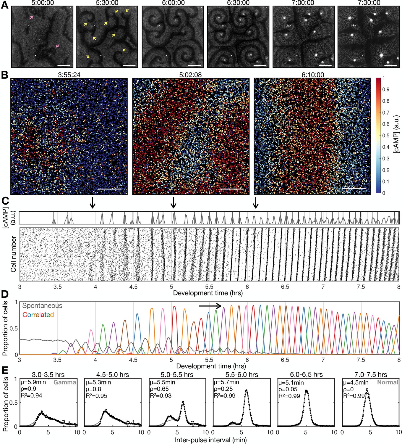
(A) cAMP waves (dark bands) imaged using the Flamindo2 reporter following starvation (for a representative movie see Figure 1—video 1). Arrows indicate circular waves (pink) and spiral waves (yellow). Scale bar: 2 mm. (B) The distribution of cells and internal [cAMP] (colour) following starvation. Scale bar: 200 µm. (C) Representative time series of the internal [cAMP] within an individual cell (top) and a plot of signal peaks for 1000 cells (bottom). (D) Changing proportions of correlated (coloured) and spontaneous (grey) activation events following starvation; each colour represents a single cAMP wave. Arrow: onset of spiral formation. (E) The distribution of inter-pulse intervals over different 30 min time intervals after starvation onset with the mean of each shown by parameter µ, together with a fitted sum of the gamma (weighted by value ρ) and normal (weighted by value 1-ρ) distribution. For the gamma distribution, the shape and rate parameter were 6.6 and 1.25 min respectively, and the mean of the normal distribution varied (from 6 to 4.5 min).

Early during development, cells predominantly fired asynchronously. The proportion of spontaneously activating cells declined as the signalling behaviour became more correlated, with periodic waves of signalling including an increasing proportion of the cells (Figure 1D). Prior to the onset of cAMP waves (around 4 hr after starvation), cells produced cAMP pulses spontaneously at a mean rate of around 1 pulse per 12 min, with a minimum of around 1 pulse per 4 min (Figure 1E). During this time, the population distribution of inter-activation intervals follows a gamma distribution (Figure 1E and Figure 1—figure supplement 1B). We interpret this fit as there being a minimum waiting time between pulses (a refractory phase), with the exponential tail of the distribution suggesting the probability of firing is independent of the previous firing event.

The initial cAMP waves (around 4–5 hr) are broad bands of broken waves amalgamating from numerous circular patterns that expand from spontaneously activating cells (Figure 1A). Activation events prior to synchronisation are spontaneous, spatially variable, and mostly do not initiate a cAMP wave. Together with the independence of successive firing events, these observations are inconsistent with the model that individual ‘pacemaker’ cells act as the organising source of global cAMP waves. However, it may be possible that cell clusters (arising for example from random motion) may collectively act as a pacemaker (Mirollo and Strogatz, 1990; Gregor et al., 2010). For example, if the cell cluster is sufficiently dense such that at least one cell in the cluster is likely to activate just after the refractory time. Nevertheless, any given cell will experience circular waves from several different sources with a variable periodicity (5–9 min).

Circular waves produce cAMP signals at irregular intervals which are typically greater than the inter-pules interval (Figure 1D). Consequently, not all cells will relay a circular wave because cells that fire synchronously with one wave can potentially reactivate and so be refractory for the next wave. This is highlighted by a multi-peaked population distribution for inter-activation intervals where the smallest peak is associated with spontaneous cAMP pulses, while the other peaks are associated with synchronised firing during a wave (Figure 1E and Figure 1—figure supplement 1B). Rotating spiral cAMP waves form from broken waves around 5–6 hr following starvation (Figure 1A). To interrogate how waves break and give rise to spiral waves, we engineered cells to express blue-photoactivable adenylyl cyclase (bPAC; Stierl et al., 2011) to control the time and place of cAMP waves by exposing a subset of cells to blue or green light (Figure 1—figure supplement 2 and Figure 1—video 3). In the absence of light pulses, we observed a steady train of periodic waves (Figure 1—figure supplement 2B). Photoactivation of a small patch of cells generated a circular wave which fused with oncoming waves (Figure 1—figure supplement 2A first and second row and Figure 1—figure supplement 2C). Wave breaks (Figure 1—figure supplement 2A forth – sixth row) occurred only when the oncoming wave collided with an asymmetric wave generated by the activated patch (Figure 1—figure supplement 2A third row). We interpret the asymmetry arising when cells activate at the border of two regions; one where cells are in a refractory state (preventing wave propagation) and the other in which cells are recovered (allowing wave propagation; Figure 1—figure supplement 2D). This experiment suggests that spiral waves might naturally arise from spontaneous cell activation behind a circular wave, where neighbouring cells are transitioning from a refractory to rest state.

Rotating spiral patterns generate waves that are more frequent and regular than circular patterns (Figure 1 5-6 hr onwards) and hence become the dominant pattern over time, overriding the less frequent circular waves, as reported in previous studies (Lee et al., 1996). The mean wave frequency steadily increased towards the maximum firing frequency of cells, around once every 3–4 min (Figure 1E). Consequently, the proportion of spontaneously activating cells tends to zero as there is no time to activate between waves (Figure 1D), and the population distribution of inter-pulse intervals tends to a normal distribution (Figure 1E). To understand the basis of the heterogeneity in inter-pulse intervals, we quantified the single-cell differences in activation times relative to the wave centre (Figure 1—figure supplement 3A, B). Aided by Markov modelling, we observed a short-term bias in firing tendencies: for example, a cell that fires ahead of its neighbours has a 60% chance of repeating this early firing, 35% chance of switching to late firing, and a 5% chance of skipping the subsequent wave (Figure 1—figure supplement 3C, D). Whether a cell fires before or after the wave does not affect its probability of skipping a wave. Overall, these data suggest no intrinsic difference between cells beyond a slight history dependence.

The onset of collective migration

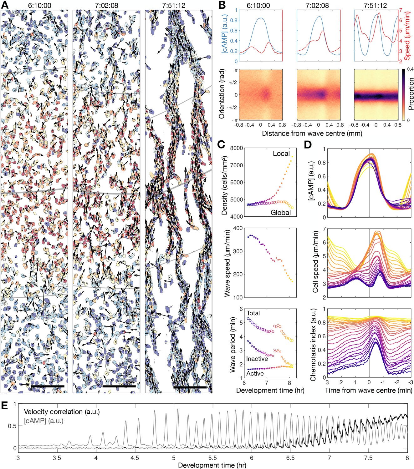
To relate how information encoded by spiral waves coordinates collective motion, we compared changes in cAMP wave dynamics to cell chemotaxis (Figure 2 and Figure 1—video 2). Chemotaxis is directed by the external cAMP concentration field, which is determined by the release of internal cAMP (reported by Flamindo2) from individual cells. The spatial organisation and motility of cells changed rapidly, occurring around 7 hr following starvation, coincident with the dominance of spiral waves (Figure 2A and Figure 2—figure supplement 1). During this process, cAMP waves steadily became more frequent, slower and thinner, and cells became faster, more directional, and persistent in their movement (Figure 2B and C). The profile of the mean cAMP pulse in single cells remained constant with each wave. Since the duration of a cAMP pulse ( $τ$ ) remains constant, and the wave speed ( $v$ ) decreases, then the wave width ( $w = v \times τ$ ) also decreases. A thinner wave generates a steeper external cAMP gradient, which may enhance chemotaxis (Song et al., 2006).

Figure 2 with 1 supplement see all

Download asset Open asset

Transition to collective cell motion.

(A) Snapshots of cell velocities (arrows) and signal states (coloured by [cAMP], as in Figure 1B) surrounding a cAMP wave (travelling from top to bottom) at three different time points following spiral wave formation. The inferred wave boundaries and peak are highlighted as grey lines. Scale bar: 100 µm. (B) Top: the mean cell [cAMP] (blue) and speed (red); bottom panels show the orientations of the cells with respect to the direction of wave motion (0 is facing the wave; ± π facing away from the wave), as a function of distance from the wave centre for the three waves shown in A. (C) The local (mean) and global population density (top), wave speed (middle), and wave period (bottom) for each wave during 6–8 hr following starvation. Each data point is coloured by wave number. (D) The mean cell [cAMP] (top), speed (middle), and chemotaxis index (bottom) across each wave, represented as the time to the wave centre (positive values correspond to behind the wave). Each line is coloured by wave number as in C. (E) The mean cell [cAMP] (grey) and local velocity correlation (black) between cells within a 400 µm² area.

To quantify collective cell motion, we used the following two measures: (i) the mean chemotaxis index, the proportion of cell movement in the direction of the oncoming wave (Skoge et al., 2014; Figure 2B and D), and (ii) the local correlation of cell velocity (De Palo et al., 2017; Figure 2E). Cells consistently moved towards the wave source at wave fronts but remained spatially uniform before 6 hr of starvation due to random cell motion at the wave rear (Figure 2B bottom left panel). This is highlighted by a peak in the local correlation of cell motion (Figure 2E) and the mean chemotaxis index (Figure 2D bottom panel) at the wave front, both of which then decay towards zero (indicating random cell motion). For infrequent, fast and wide waves (i.e. circular patterns), the chemotaxis index and local correlation of cell motion reached their baseline values at the following wave front, indicating cells move randomly. This random cell motion disrupts the order in collective cell motion initially induced by the front of the wave. For frequent, slow and thin waves (i.e. rotating spiral waves), the chemotaxis index and velocity correlation significantly change as the cAMP wave frequency increases between 6 and 8 hr following starvation. From 6.5 hr onwards, when the wave period is less than 4.5 min, the measures of collective cell motion do not relax back to their previous values by the next wave and hence gradually increase over time to constant, elevated values across the entire wave (Figure 2D and E). In parallel, the cell speed at the front of the wave increases incrementally with each wave until it peaks at around 7 µm min⁻¹ (Figure 2D second panel). These data are consistent with models where decreasing the wave period causes cells to gradually become more persistent towards the direction of the wave source and hence gain consistent collective motion (Skoge et al., 2014).

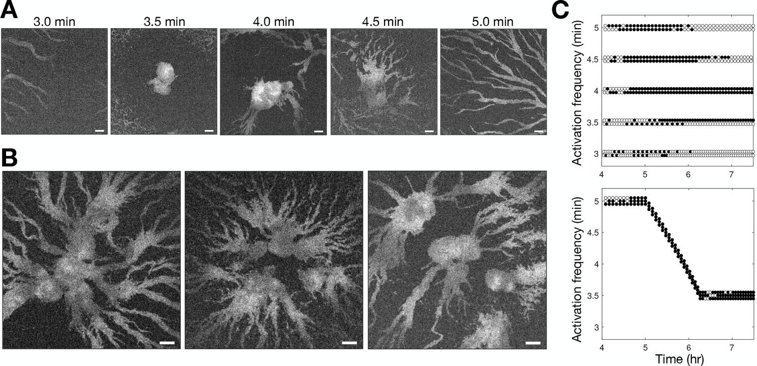
To test the relationship between wave frequency and collective migration in the full population context, we photoactivated bPAC in a small patch of cells at different intervals and monitored the resultant activation waves (Figure 3 and Figure 3—video 1). Consistent with our observations shown in Figure 2, cells collectively migrated towards the signalling centre only when the induced wave period was less than 4.5 min (Figure 3A). However, photoactivation of cells with a period less than 3.5 min did not result in aggregation. We infer that this is because cells cannot relay a steady periodic signal close to their maximum firing rate initially, resulting in a missed wave every second photoactivation event (Figure 3C), leading to the signalling centre becoming ‘taken over’ by another set of period waves. Motivated by the observed change in wave frequency during aggregation, we sought to test if it were possible to induce large cell aggregates by photoactivating cells at a faster rate than what we observe experimentally by reducing the wave period gradually from 5 min to 3.5 min from 5 to 6 hr following starvation, rather than 6–8 hr (Figure 3C second panel). This was indeed achievable, resulting in the accumulation of a significantly larger number of cells around the signalling centre and conglomerates of several aggregates (Figure 3B). These artificial signalling centres induce large aggregates by entraining the territories of neighbouring signalling centres. Our data support the notion that the increase in wave frequency is a crucial determinant of the transition to collective motion. We now turn to the question of how cells generate this increasing wave frequency.

Figure 3 with 1 supplement see all

Download asset Open asset

Controlling aggregation by setting the cAMP wave frequency.

See Figure 3—video 1 for live movies. (A) Raw images of cells subjected to 3 hr of periodic activation of the blue-photoactivable adenylyl cyclase (bPAC) (with pulses applied at centre of the field of view) at 3, 3.5, 4, 4.5, and 5 min intervals. Scale bar: 100 µm. (B) Same as A except that the frequency steadily increased from 5 to 3.5 min intervals. Note that the size of the images is larger than those in A. Scale bar: 100 µm. (C) Time series of the periodic photoactivation protocol for the experiments shown in A (top) and B (bottom). The coordinate of each circle represents the time (x-axis) and frequency (y-axis) of photoactivation, and its colour indicates whether it resulted in a relayed circular wave (black) or not (white). Experiments in A are in duplicate, and those in B are in triplicate.

Spiral wave progression

To characterise the regulation of spiral wave dynamics, we imaged and analysed the motion and signalling of individual cells around the spiral core following the onset of spiral formation. The spiral core is the region about which the spiral tip (the end of the activation wave) moves. Based on the general theory of excitable media, the spiral tip will sustain itself and the entire spiral wave by virtue of circular motion (Tyson and Keener, 1988; Winfree, 2001). In other words, the circulation of the spiral tip is the organising source of the spiral wave. To better understand the dynamics of spiral tip circulation, and how it relates to the changes in wave dynamics, we tracked the position of the spiral tip and the shape of the spiral wave from spiral formation to aggregation (Figure 4, Figure 4—figure supplement 1, Figure 4—videos 1–3). To track tip motion, we mapped the [cAMP] of individual cells to a phase variable measuring the sequence of changes in the internal [cAMP] during a cAMP pulse (Figure 4B, Figure 4—figure supplement 1B, C). During a cAMP pulse, this variable increases from 0 (baseline [cAMP]) to ±π (maximum [cAMP]) and then back to 0. This approach reveals the spiral singularity — or topological defect — which is the point in space around which cells are distributed across the full spectrum of phase states. At each time point, we estimated the spiral tip location as the mean position of maximally activated cells closest to the singularity (Figure 4B). Additionally, we fitted a spiral curve to the spatial distribution of maximally activated cells (Figure 4A and C first panel).

Figure 4 with 4 supplements see all

Download asset Open asset

Spiral tip circulation and spiral wave progression.

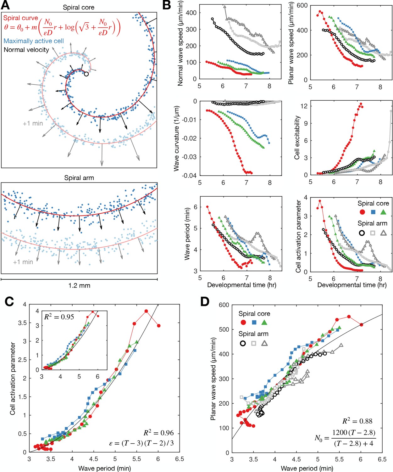
(A) The fitted spiral curve (thick line) and predicted wave boundary (thin line) with the spatial distribution of: the internal [cAMP] (first panel), the signalling phase (second panel), and maximally activated cells (phase ±π) 2 min apart (0 min – black,+2 min – grey; third panel). Scale bar: 100 µm. (B) 3 min tracks (thick black line) of the spiral tip (star) circulating around the pivotal axis (thick white circle) overlayed with cell positions and signalling phase. Scale bar: 50 µm. (C) Plots of the fitted spiral curve (mean curve per rotation; top) and track of the radius of spiral tip circulation (bottom), coloured by time since spiral wave formation. (D) Time series of the spiral tip circulation rotational period (first panel), rotational radius (second panel), and speed (third panel), in addition to the spiral curve parameter defining the fitted spiral shape in C (fourth panel) for each experiment (red, blue, and green) from the onset of spiral formation. Each circle represents the mean value per rotation and the lines represent the instantaneous values (e.g. rotational period is 2π /). See Figure 4—videos 1–3 for live cell movies.

Spiral waves significantly change in rotation rate and curvature during aggregation, which we refer to as spiral wave progression (Figure 4C and Figure 4—videos 1–3). These changes in spiral wave structure and dynamics are coupled to changes in spiral tip circulation (Figure 4B–D). Each rotation of the spiral tip generates a wave: the rate at which the activation waves circulate around the signalling centre sets the frequency of global activation waves disseminated from the signalling centre. The spiral tip rotational period decreased from 5.5 min to 3.5 min. These changes in the rotational period of the spiral tip translate to the changes in the rotation rate of the spiral wave: the decrease in the spiral tip rotation period (Figure 4D first panel) is consistent with the decrease in the wave period away from the spiral core that coincides with the onset of collective migration (Figures 2C and 3). The acceleration of spiral tip circulation is associated with spiral core contraction; the radius of circulation steadily reduced from around 100 µm to 20 µm (Figure 4D second panel). Meanwhile, during this contraction, the spiral tip speed decreased from 100 to 120 to 40–50 µm min⁻¹ (Figure 4D third panel).

How do cells at the signalling centre drive spiral wave progression? To measure the fundamental signalling parameters and how they change over time, we utilised the general theory of excitable media (Tyson and Keener, 1988). Dictyostelium cAMP waves can be shown to satisfy this theory (Tyson et al., 1989; Foerster et al., 1990). Our high-resolution datasets now make it possible to apply this theory to understand how spiral waves change during aggregation, independently of the specific equations that model cAMP release, which are still disputed (Sgro et al., 2015; Kamino et al., 2017). According to this theory, the shape of the spiral wave must satisfy a curve that is approximately Archimedean (Materials and methods, Equation 2). The spiral curve depends on a single parameter $k = N_{0} / ε D$ (referred to here as the curve parameter) which relates the signalling parameters $N_{0}$ (the planar wave speed), $D$ (the signal diffusion constant), and $ε$ (the ratio of the rates of cell inactivation and activation, which we call the cell activation parameter; Materials and methods, Equation 3). Crucially, the inverse of $ε$ is the measure of cell excitability and specifies the rate at which cells activate. By fitting the spiral curve to the spatial distribution of maximally activated cells at each time point (Figure 4A; Figure 5A, Figure 4—videos 1–3), throughout spiral wave progression, we obtain a measurement of how the cell excitability and planar wave speed change over time (Figure 5B second column). Specifically, both measures of the cell signalling phenotype can be expressed in terms of spiral wave properties that we can measure (Materials and methods, Equation 4), such as the normal wave speed and wave curvature (Figure 5B first column).

Figure 5 with 1 supplement see all

Download asset Open asset

General theory of excitable media – cell excitability is coupled to wave dynamics.

(A) Representative curve fits (red line) to the distribution of maximally activated cells (blue dots) at (top) and away from (bottom) the spiral core. The normal wave speed is shown as black arrows. (B) Time series of wave characteristics derived from A. Coloured lines show data from the spiral core. Greyscale lines show data away from the core. (C) The cell activation parameter (calculated using the eikonal relation) plotted against the wave period at the spiral core. Inset shows the same plot, but with the activation parameter derived from the curvature relation, together with the fitted quadratic function (black line). (D) The dispersion relation at (colours) and away from (greyscale) the spiral core, together with the fitted saturating function. The data shown in dark grey are derived from the same experiment shown in Figure 2. Spiral wave data is from the same experiments shown in Figure 4 (same colours).

This analysis reveals that the activation parameter and planar wave speed both decrease during spiral wave progression (Figure 5B). Firstly, we find that the planar wave speed halves in value as the wave period decreases towards its minimum (Figure 5D). The theory of excitable media provides the following interpretation: as the wave period decreases, cells have less time to reset between waves, causing slower cell activation and wave speed (the dispersion relation), which gives rise to the deceleration of wave speed during core contraction. This deceleration quantitatively matches the changing wave dynamics away from the spiral core (Figures 2C and 5B), meaning the circulation of the spiral tip determines the wave speed away from the core, in addition to the frequency. Secondly, the theory interprets the increase in spiral wave rotation rate and curvature to be a consequence of cells becoming more excitable over time (Figure 5C). In other words, the spiral waves progress because cells can activate faster. Indeed, although there was temporal variation between experimental replicates, the activation parameter collapses onto a highly consistent curve when plotted against the wave period (Figure 5C), showing how the wave dynamics are strongly coupled to the excitability of the cells. A simple quadratic provides a good fit regardless of derivation used for quantifying the activation parameter (Materials and methods, Equations 4 and 5). In summary, this analysis implies the change in cell excitability is a key element driving spiral wave progression. We now evaluate different hypotheses for mechanisms driving spiral wave progression.

Hypotheses

Hypothesis 1: increased collective excitability by cell reorganisation with constant individual excitability

The existing paradigm, based on mathematical modelling, is that spiral wave progression is driven by cell aggregation (Höfer et al., 1995; van Oss et al., 1996). In this view, an increase in cell density elevates cAMP production and degradation rates per unit volume, increasing the collective excitability around the aggregate. In this way, the spiral wave rotation rate and curvature increase as cells accumulate at the spiral core, even though the intrinsic excitability of individual cells remains constant. Consistent with this paradigm, we measured a substantial decrease in the cell activation parameter (inverse of cell excitability) and increase in cell density during spiral wave progression (Figure 6). The relationship between density and the activation parameter is incredibly sensitive, meaning slight fluctuations in density (such as occurring through random motility) would correspond to dramatic changes in the activation parameter (Figure 6C first panel). However, unlike the strong relationship between wave period and cell excitability (Figures 5C and 6C third panel), a causative relationship between density and excitability is not supported by reliable fits (Figure 6C second panel). In addition, our data show that spiral wave progression occurs prior to clear changes in cell density (Figure 6A). Specifically, spiral core contraction and the increase in rotation rate are immediate and steady for around 1.5 hr following spiral wave formation (Figure 6B second panel), while the cell density sharply increases only after around 1 hr (Figure 6B first panel) once the wave period is below 4.5 min. Indeed, the rotational period is close to the minimum value before substantial changes in density occur (Figure 6B third panel). Altogether, these observations imply that an increase in cell density is not sufficient to account for spiral wave progression, at least at the onset of collective migration.

Figure 6 with 3 supplements see all

Download asset Open asset

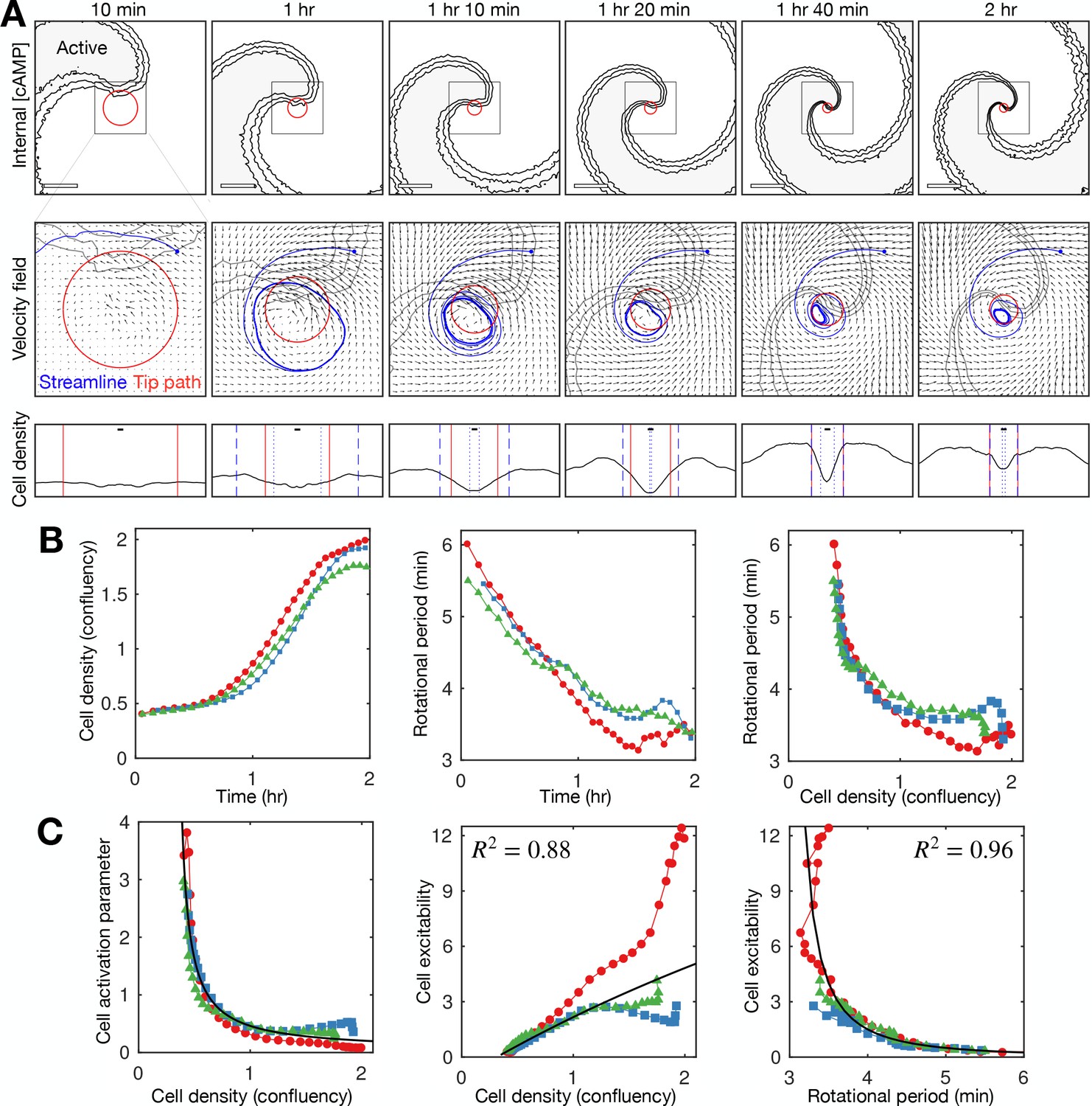
Relationship between cell density and distribution to spiral wave progression.

(A) Top row: the mean internal [cAMP] around the tip with the mean circulation radius of the spiral tip (red). Scale bar: 200 µm. Middle row: mean cell velocity field together with a representative streamline, the mean radius of the path of spiral motion (red), and contoured outline of the spiral (grey). Bottom row: cell density together with the mean radius of the spiral tip motion (red) and the minimum (dotted) and maximum (dashed) distance of the representative streamline from the axis of spiral rotation (blue). Scale bar: 10 µm (≈1 cell diameter). Each plot represents a 5 min average. (B) Time series of the cell density (fraction cell confluency, estimated with cell area of π 5² µm²) around the spiral core (first panel) and spiral tip rotational period (second panel), together with the relationship between the cell density and rotational period (third panel). Shown are the same three datasets (colours) shown in Figures 4 and 5. Data points represent average values per rotation, in contrast to Figure 4D. (C) Relationship between the cell activation parameter (first panel) and cell excitability (inverse of the cell activation; second panel) and the cell density. Relationship between cell excitability and wave period (third panel). The cell activation parameter (inverse of cell density) structured by cell density and period was fitted with a reciprocal curve ( $ε = 0.04 + \frac{0.28}{n - 0.32}$ ) and quadratic curve (same as in Figure 5), shown as black lines, with their respective R² values.

A more recent model for cAMP release (Sgro et al., 2015), which is based on the FitzHugh-Nagumo model rather than the Martiel-Goldbeter model (Martiel and Goldbeter, 1987), shows improved quantitative behaviour of cAMP release from single cells (Huyan et al., 2021). It is conceivable that incorporating this more recent model into the earlier models of spiral waves (Höfer et al., 1995; van Oss et al., 1996; Dallon and Othmer, 1997) could provide spiral wave progression consistent with our data - an increase in the spiral wave rotation rate prior to cell aggregation. To test this, we developed a hybrid partial differential equation (PDE) agent-based model (ABM; see Materials and methods and Supplementary Information) in the same vein as van Oss et al., 1996, but replacing the Martiel-Goldbeter model with the modified FitzHugh-Nagumo model. To explore how cellular reorganisation influences the signalling pattern, we fixed all signalling parameters such that the intrinsic cell excitability does not change. This model reproduced a rotating spiral wave and experimentally observed spatial patterning of cells (Figure 7, Figure 7—videos 1 and 2). In the model, the rotating spiral wave creates a limit cycle in cell motion (see the circular streamline in Figure 6A and Figure 6—figure supplement 1). Cells collect along the limit cycle via chemotaxis from both inside and outside the path of tip circulation, forming a ring pattern. The emergence of this limit cycle is matched in our data (Figures 6A and 7, Figure 6—videos 1 and 2). In data and model, both the radius of spiral tip circulation and the ring pattern of cells contract over time. In our model, this contraction occurred in the absence of cell-cell physical interactions (i.e. no crowding effects) but not in the absence of cell motion (Figure 7D and E first panel). These tests indicate that spiral core contraction can be attributed to the spatial reorganisation of cells via chemotaxis towards the circulating wave, but not necessarily due to crowding effects from cells funnelling towards the spiral core. This effect is also observed in data (Figure 6A): the limit cycle is ‘blunted’ at the location of the spiral tip, suggesting that cell chemotaxis is deflected around the external [cAMP] field of the spiral tip, inwards from the edge of the cell ring. Put simply, the tip is deflecting cells inwards.

Figure 7 with 4 supplements see all

Download asset Open asset

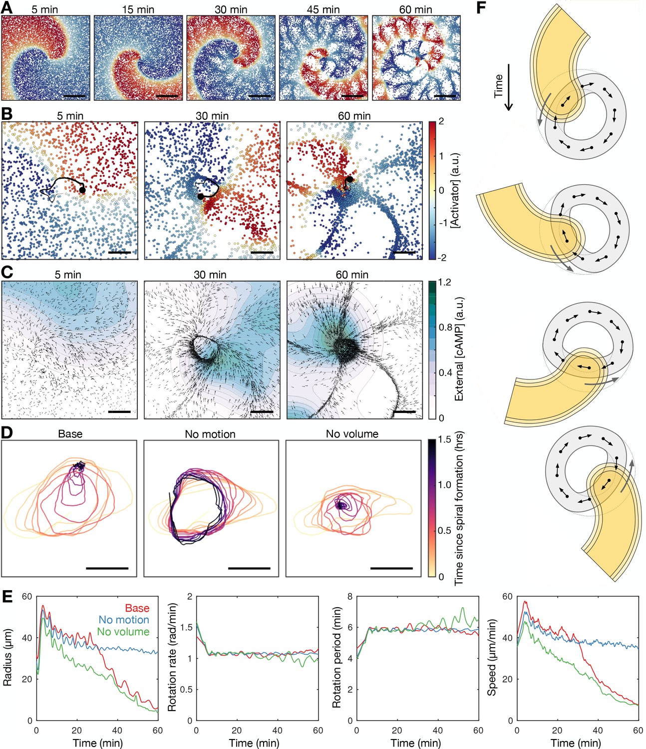
Mathematical model of spiral wave progression (constant cell excitability, variable cell density).

(A) Simulation of the cell population distribution across space and the concentration of the species governing cAMP release (colour). Scale bar: 500 µm. (B) Same as A together with the track (black line) of the spiral tip (black circle). Scale bar: 100 µm. (C) Progression of the external [cAMP] field (colour) with cell velocities (black arrows). Scale bar: 100 µm. (D) Tracks of the spiral tip (coloured by time) for the original simulation (shown in A–C), a simulation without cell motion (second panel) and without cell volume (third panel). Scale bar: 50 µm. (E) Time series of the spiral tip circulation radius, rotation rate, rotation period, and speed for the simulated tracks presented in D. (F) Schematic of the mechanism of spiral tip contraction; as the spiral tip travels around the ring pattern of cells (grey), its external [cAMP] field (yellow) directs cell motion (black arrows) inwards from the ring tangent, resulting in the deformation of the cellular ring.

Since our data point to the contraction of the radius of spiral tip circulation as the driver of spiral wave progression (Figure 4B–D), our model suggests the following scenario for the progression of the spiral wave: as the external [cAMP] field of the spiral tip rotates about the spiral core, it draws cells from the cellular ring inwards, causing a decrease in the circulation radius hence an increase in the rotation rate. In this view, the spiral progression associated with the onset of collective chemotaxis is driven by spiral core contraction. This contrasts the original formulation where cell reorganisation increases the cell density, which increases the collective excitability.

This contraction scenario sufficiently explains spiral core contraction but not spiral wave progression. Specifically, the spiral wave does not increase in rotation rate during spiral core contraction (Figure 7E second and third panel). The speed of spiral tip motion decreases too much to offset the contraction in the radius of circulation (Figure 7E fourth panel). This is a flaw in the model since the increase in wave frequency is the key element of change coinciding with the onset of collective cell migration. By adding an additional component to the model, which allows the excitability of individual cells to increase over time, this flaw can be bypassed, with the model outputting a strong increase in wave frequency (Figure 7—figure supplement 1 and Figure 7—video 3).

Hypothesis 2: increased individual cell excitability driven by wave dynamics

An increase in cell density is not sufficient to explain spiral wave progression. This suggests that spiral wave progression does not arise because of the increase in collective excitability resulting from aggregation, but cells become more excitable individually. How would this increase in individual cell excitability occur? Based on the relationship in Figure 5C, we propose that individual cell excitability (i.e. the rate of cell activation) increases as the wave period decreases. That is, cell excitability is coupled to the wave dynamics. This hypothesis states that spiral wave progression is due to positive feedback between cell excitability and the activation wave period: in the context of the spiral wave, which generates periodic waves, the excitability of cells increases the rotation rate of the spiral wave, thereby decreasing the wave period, which raises cell excitability and so forth.

Due to the conservation of the rotational period at the signalling centre and wave period away from the signalling centre, one consequence of Hypothesis 2 is that cell state should be similar across the field. To test this property, we used the quadratic relationship between the cell activation parameter and wave period (Figure 5C) to rederive the relationship between the planar wave speed and wave period (the dispersion relation) in a different context – away from the spiral core. To measure the wave dynamics and structure away from the spiral core (Figure 6B), we exploited that the spiral curve approaches a circle distant from the core (Figure 6A) and fitted an equation for a cone to the time evolution of the spatial distribution of maximally activated cells (Materials and methods). Using this approach, we find a consistent dispersion relation both at and away from the spiral core (Figure 5D). In other words, the changes in cell state due to wave dynamics are the same across the population. This match was critically dependent on the relationship between cell excitability and wave period that is stated in Figure 5C.

To test whether the coupling of excitability to the wave dynamics sufficiently describes spiral wave progression, we modelled cAMP spiral waves at constant cell density, with the intrinsic excitability of cells changing in response to external cAMP (Figure 8 and Figure 8—video 1). The earlier models analysed by Höfer et al., 1995 and van Oss et al., 1996 were based on the spatial continuum extension of the Martiel-Goldbeter model analysed by Tyson et al., 1989. The key extension to the Tyson model by Hofer/van Oss is that the cell density can change. By using the Tyson model, we return to the original formulation, but instead of allowing density to change, we couple cell excitability to the cAMP wave dynamics. We set the cell activation variable to be a simple time-dependent function where the variable tends to a baseline value and decreases in response to external [cAMP] (Materials and methods). Figure 8A shows the time evolution of the simulated spiral wave. This solution reproduces features of spiral wave progression such as the rate of spiral core contraction (Figure 8B), increase in spiral wave curvature, increase in the spiral rotation rate, and the coupling between the cell activation parameter and the wave period (Figure 8C). The similarity between our experimental data and this model (even with parameter values rounded to the nearest order of magnitude) suggests that the positive feedback between cell excitability and the wave period is a sufficient mechanism driving spiral wave progression (Figure 8—figure supplement 1).

Figure 8 with 3 supplements see all

Download asset Open asset

Mathematical model of spiral wave progression (constant cell density, variable cell excitability).

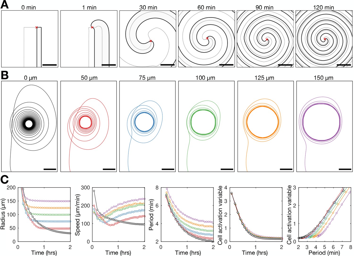
(A) Numerical solution depicting the spatial distribution of the external [cAMP] (black contour with shaded interior, $u = 1$ ) and the inactivator species (grey contour $v = 0.6$ ). Also shown is the spiral tip location (red cross) estimated by the contour intersections. (B) Path of spiral tip circulation without (black) and with (colours) a physical block of various sizes (radii shown above). Scale bar: 100 µm. (C) Time series of the spiral tip circulation: radius (first panel), speed (second panel), rotation period (third panel), and the cell activation variable (fourth panel). Also shown is the relationship between the cell activation variable and wave period (fifth panel). The colours represent the measures of circulation for the differently sized physical blocks shown in B.

Lastly, the general theory allows us to predict the radius of spiral tip circulation from the measured cell excitability (the curvature relation, Materials and methods Equation 5). Is the change in cell excitability driving the change in circulation radius (Hypothesis 2) or is the radius driving the change in excitability (Hypothesis 2)? If Hypothesis 1 was true, then a change in the measured radius of circulation should precede the change in excitability and hence the predicted radius. In Hypothesis 2, the circulation radius adapts to changes in cell excitability, in line with previous experiments using caffeine, which inhibits cAMP relay (i.e. reduces excitability), caused a larger radius of circulation (Siegert and Weijer, 1989). Further supporting Hypothesis 2, our data show the change in predicted radius precedes the change in the measured radius, with convergence at the end of spiral wave progression (Figure 5—figure supplement 1). That is, the radius of spiral tip circulation is a consequence, not driver, of spiral wave progression.

Exploring the properties of the radius contraction in the adapted Tyson model shows that the inclusion of a hole in the cell density field does not hinder spiral wave progression. The spiral wave becomes pinned to the hole, which sets the minimum radius of spiral tip circulation (Figure 8B and Figure 8—video 2). The wave period reduces (Figure 8C third panel) because the speed of the spiral tip speed remains elevated (Figure 8C second panel) by virtue of an increase in excitability (Figure 8C fourth and fifth panel), compensating for a large radius of circulation (Figure 8C first panel). This simulated result contrasts Hypothesis 1, suggesting that preventing core contraction does not impede spiral wave progression.

Hypothesis testing

We have investigated two hypotheses for spiral wave progression. The prevailing paradigm (Hypothesis 1) is that excitability increases due to an increasing cell density; however, this model is not supported by our data comparing density with wave period and excitability (Figure 6). Our reformulation of this hypothesis predicted that cell rearrangements drive the increase in the spiral wave rotation rate via contraction of spiral tip circulation (Figure 7). In contrast, Hypothesis 2 proposes that the wave dynamics change cell excitability (Figure 8). The key difference between these hypotheses is that in Hypothesis 1, spiral tip contraction is the driver of spiral progression (Figure 7F), whereas in Hypothesis 2, contraction is a consequence (Figure 8—figure supplement 1). Exploring the properties of the models underlying these hypotheses provides a clear experimental test: to constrain the radius of spiral tip circulation.

To experimentally test the competing hypotheses, we imaged Dictyostelium aggregation in the presence of physical blocks (low melt agarose particles with radii ranging between 25 and 150 µm; Figure 9 and Figure 9—video 1). Spiral waves can become pinned to the blocks (Figure 9A), with their minimum radius of circulation set by the block radius (Figure 9B). Spiral waves that are pinned to a block cannot fully contract (Figure 9C first panel) but nevertheless undergo a steady increase in rotation rate and hence decrease in wave rotational period (Figure 9C third panel). The circulation rate increases because the spiral tip speed does not decrease to the same extent as the unconstrained spirals (Figure 9C second panel). This observation is in agreement with the model simulations shown in Figure 8, revealing the same effects as in the data – wave speed increased to compensate for larger radius of circulation, generating a reduced rotational period. This observation also reflects our simulations predicting that spiral waves can progress in the presence of physical blocks due to a coupling between the cell excitability and wave dynamics. In addition, this coupling between wave frequency and excitability is also apparent in our photoactivation experiments, in which a gradually increasing pulse frequency enhanced aggregate formation (Figure 3). Together, these observations are consistent with Hypothesis 2, but not Hypothesis 1: the contraction of the spiral tip circulation is a consequence, not a driver, of spiral wave progression.

Figure 9 with 1 supplement see all

Download asset Open asset

Physical occlusion of spiral core.

See Figure 9—video 1 for live cell movie. (A) Top: raw images of the population distributed around a physical block (dashed circle) with the spiral tip (green dot) and its track (blue line). Bottom: the spatial distribution of the internal [cAMP] with the spiral tip (black) dot and its track (black line). Scale bar: 100 µm. (B) Tracks of the spiral tip position for physical blocks of various sizes (radii shown in titles). The control case (no physical block, black) is from a dataset shown in Figures 3—5. (C) The spiral tip circulation radius (first panel), speed (second panel), and rotation period (third panel) around physical blocks with different average radii (dashed lines). Also shown is the mean (three experiments) of the control data without blocks shown in Figures 3—5 (black). Panel 2 also shows the predicted speed (dashed lines) corresponding to the maximum rotation rate 3.5π/6 around the block radius.

Overall, our approach provides a clear interpretation of our data that spiral wave progression results from positive feedback between cell excitability and wave frequency, arising only in the context of the spiral wave pattern (Figure 8—figure supplement 1). That is, from the initial symmetry breaking event (Figure 1—figure supplement 2), the formation of a rotating spiral wave produces stable periodic activation waves that increase cell excitability, then increases the spiral rotation rate and hence wave frequency, which then feedback onto further increases in cell excitability.

Destabilisation of the spiral wave

To conclude, we now describe the cAMP wave dynamics following aggregation. As development proceeds, more and more cells move into the aggregate. Previous studies show the activation waves are organised as a multi-armed spiral in aggregates (Siegert and Weijer, 1995). How does this continued cell accumulation affect the cAMP dynamics at the signalling core and, consequently, the encoding of information by cAMP waves?

To characterise the single- to multi-armed spiral transition, we monitored the structure and dynamics of the activation waves following ring collapse (Figure 10, Figure 10—figure supplement 1 and Figure 10—video 1). Single-armed spirals destabilise only once the cellular ring fully contracts. Contraction results in a phase singularity (convergence of all signalling phases) that is fixed at the aggregate centre (Figure 10—figure supplement 1A). The phase singularity and spiral wave are unstable and disintegrate over time. This is likely because the cells are not infinitely small and can only be in one signalling phase at a time. In other words, the cells at the centre cannot activate at a rate necessary to support the full spectrum of signalling phases. The destabilisation process begins by cells signalling out-of-phase with the spiral wave, resulting in the emergence of transient patches of cell activation that gradually increase in number, size, and lifetime (Figure 10, around 2 hr following spiral formation). These activation patches rotate about the aggregate while fusing with, and breaking apart from, other activation patches and the original spiral wave, which progressively disintegrates (Figures 10A and 2–3 hr following spiral formation). This process concludes with the appearance of three stable, slow-moving and uncurved activation waves that rotate about the same fixed point at the aggregate centre (Figure 10A, from 3 hr following spiral formation). At this point, the signalling regime can be classed as a multi-armed spiral. Although the ring has collapsed, the centre of the aggregate contains relatively few cells (Figure 10—figure supplement 2). At this point, there is no phase singularity: the few cells that occupy this central region appear to have signalling phases that are uncorrelated with each other and the surrounding multi-armed spiral wave (Figure 10—figure supplement 1 – last panel). This central region of uncorrelated signalling phases is characteristic of theoretical chimera spiral waves (Totz et al., 2018).

Figure 10 with 3 supplements see all

Download asset Open asset

Transition from the single- to multi-armed spiral wave.

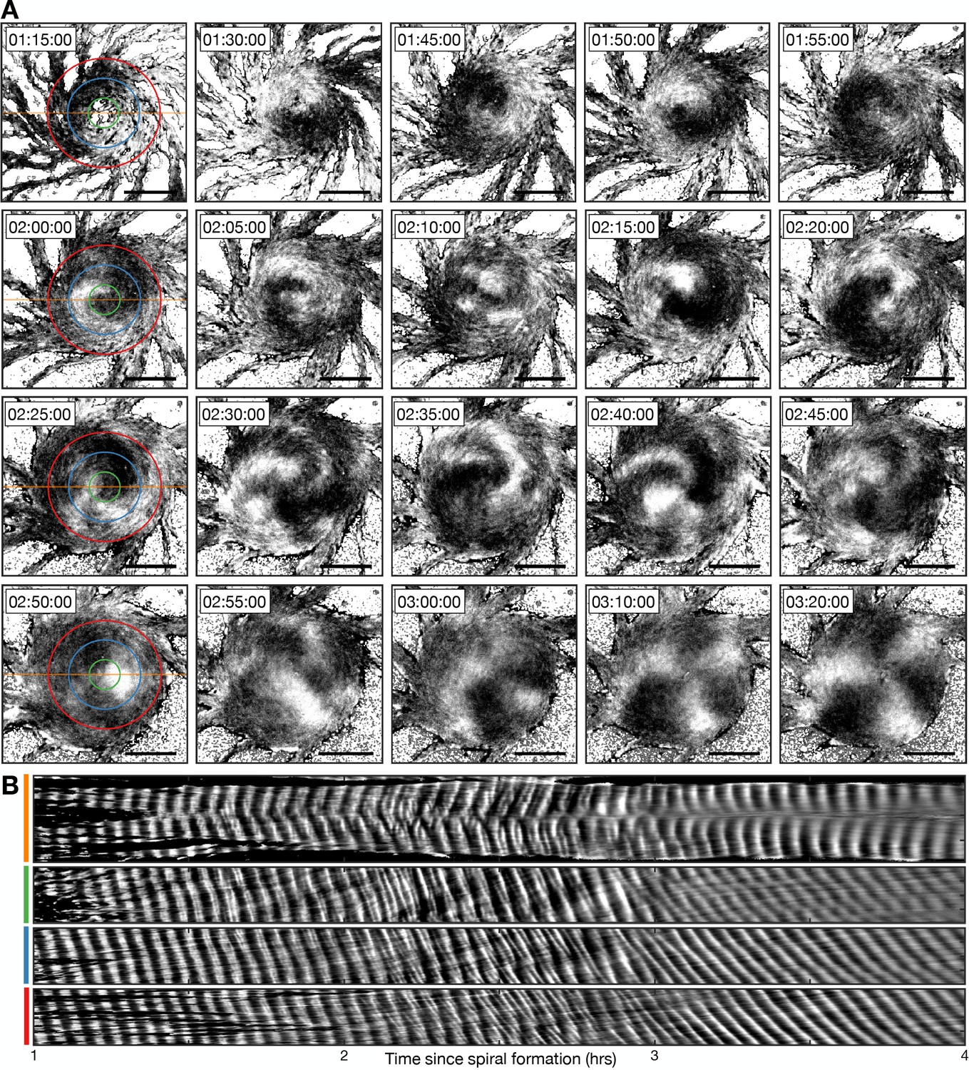
(A) Representative intensity-normalised images of the internal [cAMP] (dark - high, light - low) distributed across cellular aggregates at various time points (labelled) following spiral formation. The images in the left column are annotated with the curves from which the kymographs in B are derived. Scale bar: 100 µm. (B) Kymographs of the data presented in A along a cross-section through the aggregate centre (yellow) and circles with radius 30 µm (green), 70 µm (blue), and 110 µm (red).

To analyse the transition from the single- to multi-armed spiral, we generated a set of kymographs of cell activation states across the aggregate: one that is cross-sectional and the others that are circular (Figure 10B). The cross-sectional kymograph shows a disordered signalling regime between 2 and 3 hr following spiral formation, from around 45 min after cellular ring closure. In the circular kymographs, both the single- and multi-armed spiral waves appear as diagonal lines across space and time (<2 and >3 hr), meaning a constant rotation rate. These data show that the single-armed spiral (<2 hr) has a rotational period of 3.4±0.2 min (the minimum cell firing period, see Figures 1, 3 and 4), which is three times faster than the three-armed spiral whose rotational period is 10.1±0.7 min and wave period is 3.3±0.5 min. This means that the overall frequency with which a cell experiences a wave is the same because the three-armed spiral provides three waves in its longer rotation period. As such, the frequency of cAMP waves disseminated from the signalling centre, along the streams, remains the same for both signalling patterns. That is, both patterns encode the same temporal information.

Slow- and fast-waves coexist at the outside of the aggregate midway through the transition to the multi-arm spiral. This is visualised as a mixture of lines of two different gradients in the kymograph (Figure 10B, fourth panel, 2–3 hr). This observation suggests that both signalling regimes coexist by the mixing of cells that relay either the single- or multi-armed spiral wave. The multi-armed spiral wave eventually becomes dominant as the proportion of cells that relay the single-armed spiral wave declines. Altogether, our data suggest that the signalling pattern adapts to the change in aggregate geometry while maintaining an active phase wave that generates waves at the maximum frequency.

Discussion

To determine the properties of signal coding during signal relay, we have carried out a characterisation of collective signalling and cell motion during Dictyostelium morphogenesis. Our analysis shows how cell aggregation is coordinated by the dynamics of circulating waves of cell activation at the signalling centre. The circulation rate modulates the speed, frequency, and width of long-range periodic activation waves, spatially organised as a spiral. Leading up to aggregation, the circulation rate of the spiral tip gradually increases, resulting in an increase in the global wave frequency and a decrease in wave speed by virtue of the spiral wave rotating faster and becoming more curved. Using the general theory of excitable media, mathematical modelling, and physical perturbations of population structure, our data imply the increase in the circulation rate arises due to positive feedback between the cell signalling pattern and cell signalling state. Specifically, the wave circulation rate is determined by the ability of cells to relay the signal (cell excitability), whilst the ability to relay increases as the circulation rate increases. As such, the information encoding a morphogenetic transition unfolds from positive feedback between the signalling pattern and the cell signalling properties at the signalling centre. Altogether, our results describe how the collective behaviour of 10⁵–10⁶ cells across several millimetres is organised by circulation of a self-sustaining signal over 10²–10³ cells.

This study distinguishes biological activation waves from those produced by idealised mathematical models and chemical reactions (Winfree, 1972). The difference is that biological activation waves can encode information that can be modulated and translated to changes in the spatial organisation and gene expression of individuals beyond the spatial scale of the individual, which can feedback to changes in activation wave dynamics and structure. For Dictyostelium aggregation, information is generated locally by the rate of circulation of the spiral tip and decoded globally by cell chemotaxis. Here, by information, we mean the properties of the periodic waves, such as frequency and speed, which are translated by cells into a chemotactic and/or gene regulatory response. Information decoding via cell chemotaxis has been studied at both the single cell and population levels. There are several contrasting views regarding the wave properties which cells interpret for chemotaxis. One view is that the ability for cells to move collectively increases with an increase in wave frequency. Skoge et al., 2014 showed, by controlling the frequency of cAMP waves, that the chemotactic index increased as the frequency became maximal (Skoge et al., 2014). This observation is consistent with both our correlative and optogenetic data showing onset of collective migration as the wave frequency approaches the maximum cell activation rate. An alternative view is that cells ‘count’ waves: artificial rotating waves revealed that 4–5 waves at high frequency can induce cell polarity migration (Nakajima et al., 2016). While we cannot rule out a counting mechanism, based on our data here and early data on population measurements of aggregation, in which cells would be counting upwards of 30 waves before making the decision to collective migrate, any counting mechanism would be context-dependent, for example, using counts above a certain frequency of pulses. An alternative view is based on the wave gradient, where cells move maximally towards steep stationary (Fisher et al., 1989; Song et al., 2006) and/or increasing (Varnum et al., 1985; Wessels et al., 1992; Nakajima et al., 2014) gradients over time. Again, this view is consistent with our data, where both the wave speed and width decrease as the wave frequency increases, meaning that cells are exposed to a steeper gradient for a longer time. Overall, these different mechanisms are looking at different properties of the wave. What our study shows is that all the wave properties: speed, frequency, and width are specified by the circulation of the spiral tip. Specifically, once the frequency is set by the tip, all other features are set by default. Altogether, our study implies that the circulation rate of the signal at the signalling centre is the mechanism of information production, regardless of the specific information-decoding mechanism.

The mechanism by which cell state changes in response to the changing wave dynamics is explained, at least in part, because information contained within periodic waves is also decoded in terms of gene expression. In Dictyostelium, and many other systems, gene expression is responsive to the frequency of signalling. Expression of pdsA, which encodes a cAMP phosphodiaterase, and csaA, which encodes a cell-cell adhesion protein, is sensitive to the changing frequency of cAMP pulses (Masaki et al., 2013; Corrigan and Chubb, 2014). The csaA gene is induced during infrequent cAMP signalling, then inactivated as the pulse frequency increases as cells aggregate. The transcription factor GataC displays rapid shuttling between the nucleus and cytoplasm in response to external cAMP oscillations (Cai et al., 2014). This process is low-pass filtered, with nucleocytoplasmic shuttling occurring only when external cAMP oscillations reach a threshold frequency. Here, we describe a mechanism controlling a gradual increase in the global wave frequency. In the light of these findings, it is conceivable that Dictyostelium use high- and/or low-pass filtered transcription factors to exploit the gradual increasing wave frequency to control the timing of gene activation. In this way, the sequential timing of activation of several transcription factors across the cell population can be coordinated by signalling centres that disseminate periodic waves that steadily change frequency over time. A change in cell excitability could also arise independent of changes in gene expression. For example, we can imagine a scenario in which the degradation of cAMP cannot keep up with the increased wave frequency. In this situation, the baseline cAMP increases over time.

In Dictyostelium, the temporal coding of cAMP waves allows cells to sense the extent of cell aggregation through the frequency of activation waves produced by the aggregate, which increases as aggregation progresses. In other words, the temporal code allows for long-range sensing of aggregate progression, which can be interpreted as a non-local quorum sensing mechanism. A potential advantage of this adaptive information coding system is that by moving only towards highly frequent and consistent cAMP waves, effort is then concentrated on migration directed only towards an established signalling centre. If cells were to move maximally towards each initial wave, they would meander and unnecessarily expend energy while cAMP waves settle to a stable pattern, in addition to missing out on the opportunity to chemotaxis towards sources of nutrition.

Our data reveals the transition from the single- to multi-armed spiral wave during aggregate progression (Agladze and Krinsky, 1982). In the established aggregate, the single-armed spiral is associated with an unstable signalling phase singularity at the aggregate centre. The multi-armed spiral lacks a clear singularity and instead is associated with relatively small numbers of desynchronised cells at the spiral core. This is the hallmark of the chimera spiral state, a phenomenon yet to be observed in a biological system (Totz et al., 2018). Overall, we view the transition to the multi-armed spiral as an adaption to the change in aggregate geometry to maintain an active phase wave at the signalling centre that generates activation waves at the maximum frequency.

In their physiological context, most cell populations, including Dictyostelium, are structured in three spatial dimensions. It is not trivial to extrapolate our findings (in the standard 2D plane context) to understand three-dimensional activation waves, owing to the limitless number of self-sustaining wave patterns—the scroll waves—afforded by the extra spatial dimension (Siegert and Weijer, 1992; Winfree, 2001; Durston, 2013). To better understand how biological signals are assembled, sustained, and controlled in a more general class of tissues, it would be important to extend the experimental, computational, and mathematical approaches outlined in this study to characterise the structure, dynamics, and biological effects of cAMP wave patterns that coordinate Dictyostelium morphogenesis in 3D.

Materials and methods

Generation of cell lines

Request a detailed protocol

Dictyostelium AX3 cells were engineered to express Flamindo2 and H2B-mCherry from safe-haven genomic locations for stable and uniform expression. Flamindo2 is a cAMP biosensor (Odaka et al., 2014; Hashimura et al., 2019) with a fluorescence intensity that is inversely proportional to internal cAMP levels. A codon-optimised sequence encoding the Flamindo2 reporter was knocked-in to the act5 locus for stable and uniform expression (Paschke et al., 2018; Tunnacliffe et al., 2018). H2B-mCherry, knocked into the rps30 locus, labels the nucleus for cell tracking at highcell densities (Corrigan and Chubb, 2014). For optogenetic activation of cAMP signalling, we used the light-activatable adenylyl cyclase, bPAC (Stierl et al., 2011). A codon-optimised bPAC cDNA was cloned into the extrachromosomal expression vector, pDM1203, then transfected into the act5-Flamindo2 cells.

Cell handling

Request a detailed protocol

Cells were grown at 22°C in 12 ml of Formedium HL5 medium supplemented with penicillin and streptomycin in 10 cm tissue culture dishes. Cultures were diluted to 25% of their density each day to stop cell entry into stationary phase. Cells were not used beyond 9 days of culture. For development, log-phase cells at 80% confluency were washed and resuspended in KK2 (20 mM KPO₄ pH 6.0) and then plated on 1.5% agar at between 4×10³ and 5×10³ cells mm⁻². After 1 hr in a humidified chamber, a 1.2 cm × 1.2 cm slab of agar was cut and gently placed cell-face-down onto a glass imaging dish (Bioptechs deltaT) and then immediately submerged in silicon oil to prevent desiccation. To incorporate physical blocks into the cell aggregation field, we sprinkled low-melting point agarose powder onto the KK2 agar bed before the agar had set.

Cell imaging

Request a detailed protocol

Cells were imaged at 22°C on a custom-built inverted wide field microscope (Cairn Research) with 470 nm and 572 nm LED light sources (Miermont et al., 2019). This was equipped with a Prime 95B CMOS camera (Photometrics) and 10× UplanFL N objective (Olympus). A 1.2 mm × 1.2 mm area was imaged at resolution 1 µm² per pixel every 4 s for 8 hr from 2 hr after starvation. Frame stitching was used to expand the effective field-of-view size. To image cell motion and signalling about the spiral core, including the experiments with the physical block, we imaged a 1.2 mm × 1.2 mm area for 2 hr following from 5 to 6 hr after starvation. For this, we monitored cAMP wave patterns in real time and identified waves that had started to rotate about an axis.

Photoactivation

Request a detailed protocol

For light activation of cAMP signalling, we used bPAC-expressing act5-Flamindo2 cells and a 3i spinning-disk confocal microscope with a 10× objective and Prime 95B CMOS camera (Photometrics). To initiate periodic cAMP waves, cells contained within a circular area with a ≈100 µm diameter were pulsed with 488 nm light for 1 s, at intervals to mimic physiological cAMP pulsing. Flamindo2 images (excitation 515 nm) were collected throughout the pulse sequence, every 5 s. To initiate a rotating spiral wave, we repeated the photoactivation protocol above, except that cells were photoactivated at operator-controlled points in time and space. We monitored waves in real time and identified periodic waves away from the signalling centre (around one per 5 min, 5 hr following starvation). To induce circular wave patterns, we photoactivated cells around 3 min after the previous wave. To induce asymmetric wave patterns (resulting in the broken and hence spiral wave), we photoactivated around 2 min after the previous wave.

Cell tracking and measuring cell signalling states

Request a detailed protocol

The following image analysis pipeline was implemented in Matlab 2020b. To track the position of individual cells from image sequences, the IDL particle tracking algorithm (Crocker and Grier, 1996) was applied to the cell nuclei channel (H2B-mCherry) of the image time series. The velocity of each cell at each time point was estimated by the first derivative, second order, central finite difference of cell position. To measure the mean fluorescence intensity of each tracked cell, watershed segmentation (the Fernand Meyer algorithm) seeded from the tracked cell positions was applied to the cell body channel (Flamindo2). To infer internal cAMP levels (non-dimensional), the tracked mean fluorescent intensity of each cell was normalised and smoothed using Matlab’s Savitzky-Golay finite impulse response smoothing filter. Two measures were used to identify cAMP pulses: (i) the similarity between the normalised intensity and a square pulse of length 2 min and (ii) the signalling phase $φ$ . Variable $φ$ was estimated by stratifying the time series of the internal cAMP level $c$ by its time derivate $\dot{c}$ (estimated by the first derivative, second order, central finite difference). The value of $φ$ is set as the angle around the point $c = c^{*}$ and $\dot{c} = 0$ :

φ = 2 \tan^{- 1} \frac{c - c^{*}}{c + \sqrt{{(c - c^{*})}^{2} + c^{2}}}

In addition to the time series of the inferred cAMP levels, we recorded the time points of the maximal cAMP level during each pulse, and the time points of cell activation ( $\dot{c} > 0$ ) and deactivation ( $\dot{c} < 0$ ), measured by the time point where the cAMP levels are half-maximal.

To quantify the internal [cAMP] signalling and phase field following aggregation, we tracked the fluorescence intensity of each individual pixel as a function of time, over the entire 2D image sequence. The fluorescence intensity time series was oscillatory and typically increased over time due to cell crowding. We used Matlab’s Savitzky-Golay finite impulse response smoothing filter to separate the oscillatory and background component of the signal. The background component was used to estimate the cell density of the aggregate. The oscillatory component was used to estimate the spatial distribution of signalling states and phases across the aggregate, using the same technique described above.

Activation wave curve fitting

Request a detailed protocol

To quantify the evolving dynamics of the spiral wave from cell track data, we first estimated the location of the spiral phase singularity at each time point as the central point of a circular region of radius 100 µm with the largest variance in internal [cAMP] across each cell. The location of the spiral tip was estimated by the mean position of five maximally activated cells closest to the location of the phase singularity. We estimate the axis of rotation at each time point by fitting a circle to the track of the spiral tip, half a revolution backwards and forwards in time. Using the Matlab function ‘fit’, we fit the spiral curve given by Equation 2 (see below) to the spatial distribution of maximally activated cells, starting from the axis of spiral tip circulation (Tyson and Keener, 1988). To achieve this, we determined the magnitude ( $r$ in Equation 2) and orientation ( $θ$ in Equation 2) of the vector extending from the axis of spiral rotation to the location of each maximally active cell. This fit provides the spiral orientation ( $θ_{0}$ in Equation 2) and curve parameter ( $k$ in Equation 2).

Away from the spiral core, the time and place of activation for each cell were clustered in three dimensions (two spatial and one temporal) using the DBSCAN (density-based clustering of applications with noise) algorithm as a means to identify cells with correlated signalling states (e.g. during the propagation of cAMP waves) and also, by exclusion, the cells that activate independently. This approach reveals the clusters of cell activation associated with each cAMP wave. For each wave, we estimated the dynamic curve of the wave by fitting an equation for a cone ( $t - t_{0} = N r, r = \sqrt{{(x - x_{0})}^{2} + {(y - y_{0})}^{2}}$ , where $t_{0}$ and ${(x}_{0}, y_{0})$ is spatiotemporal origin of the wave) to the time evolution of the spatial distribution of maximally activated cells. The slope of each of the cones fitted to the spatial distribution of maximally activated cells at each time point was used to deduce the speed of each wave.

Quantifying cell motion

Request a detailed protocol

To estimate the mean cell velocity field and density around the spiral wave, we measured the mean velocity and total number of cells at regular lattice areas (step size 10 µm) in the reference frame that rotates with the fitted spiral parameter $θ_{0}$ (Figure 6—video 2). The streamlines across this field were analysed using the Matlab function ‘streamlines’.

To analyse the behaviour of single cells during stable periodic waves, the fitted cone equations were used to estimate the mean internal [cAMP] and velocity of each cell as a function of distance from the wave centre. This allows an estimation of measures such as the angle difference between the direction of wave travel and cell motion, for each cell:

\cos^{- 1} (\hat{v_{i}} \cdot \hat{\hat{w}} (X_{i}))

where $\hat{v_{i}}$ is the normal velocity of cell $i = 1, \dots, N$ , and $\hat{w} (X_{i})$ is the normal velocity of the cAMP wave at the location of cell $i$ , $X_{i}$ . The following two formulae were used to measure collective cell motion: (i) the mean chemotaxis index (the proportion of cell movement in the direction of the oncoming wave) as a function of distance from the wave:

\frac{1}{N_{Ω_{j}}} \sum_{i \in Ω_{j}} \hat{v_{i}} \cdot \hat{\hat{w}} (X_{i})

where $Ω_{j}$ represents the subset of cells (subset size $N_{Ω_{j}}$ ) located at a distance $j \times 10$ µm ( $j = \dots - 1,0, 1, \dots$ ) from the wave centre, and (ii) the local correlation of cell velocity:

\frac{1}{N} \sum_{i} \frac{1}{N_{Φ_{i}}} \underset{}{\sum_{j \in Φ_{i}} \hat{v_{i}} \cdot \hat{v_{j}}}

where $Φ_{i}$ denotes the subset cells (subset size $N_{Φ_{i}}$ ) within a 50 µm radius of cell $i$ (De Palo et al., 2017). Local cell density was measured by the mean density of cells within a 60 µm radius of each cell.

General theory of excitable media

Request a detailed protocol

This section outlines the elements of the theory we have used, and we used these to interpret spiral wave progression (Tyson and Keener, 1988; Winfree, 2001).

The eikonal relation dictates how the normal speed along the wave front $N$ changes due to wave curvature $K$ :

N = N_{0} + ε D K,

where $N_{0}$ is the planar (no curvature) wave speed, $D$ is the signal diffusion coefficient (which we assume remains constant), and $ε$ is the ratio of the rates of cell inactivation and activation (which we call the cell activation parameter; Keener, 1986). For a wave extending to the pivotal axis, the solution to Equation 1 is accurately approximated by the following curve (in polar coordinates, $x = r \cos θ (r, t), y = r \sin θ (r, t)$ ):

θ \approx θ_{0} (t) + m (k (t) r + \log (\sqrt{3} + k (t) r)),

where $m$ is a constant. Parameter $k$ (the curve parameter) defines the curvature of the wave, and $θ_{0}$ is the spiral angle of rotation, with rotation rate, ${ω = \dot{θ}}_{0}$ (Tyson and Keener, 1988). We fit Equation 2 to the spatial distribution of maximally activated cells at each time point, throughout the entire progression of the spiral wave. The fit is accurate for all time points, which validates the use of the theory of excitable media even though cells are discretely distributed across space. This fit provides a measurement of the time evolution of the curve parameter $k$ , rotation rate $ω$ , and hence the wave period $T = 2 π / ω$ (Figure 4D). The value of $k$ relates the planar wave speed to the cell excitability:

k = \frac{N_{0}}{ε D},

Substituting Equation 3 into Equation 1 for $N_{0}$ allows the cell activation parameter $ε$ and planar wave speed $N_{0}$ to be expressed in terms of variables that can be directly measured from data:

ε = \frac{1}{D} \frac{N}{k + K}, N_{0} = \frac{N k}{k + K} .

Consistent with the traditional paradigm of spiral wave progression (Höfer et al., 1995; van Oss et al., 1996), we find that the cell activation parameter, which is the inverse of cell excitability, decreases during spiral wave progression (Figure 5). This result illustrates how we can identify key signalling properties of the cells from their population signalling patterns, at each time point during aggregation. Plotting $N_{0}$ from Equation 4 against the wave period $T$ provides a prediction of the dispersion relation, which quantifies how a decrease in wave period reduces the wave speed because cells do not fully reset between waves, causing them to activate slower. The curvature relation describes the relationship between radius and rate of circulation of the spiral tip:

ε = \frac{ω}{D Ω (k, r_{0})}, Ω = \frac{k (1 + 4 k r_{0} - \sqrt{1 + 8 k r_{0}})}{4 r_{0} (1 + k r_{0})},

where $r_{0}$ is the radius of spiral tip circulation, which can measure from our data (Tyson and Keener, 1988). In support of our approach, the curvature and eikonal relations produce similar values of the cell activation parameter at all time points. We use the curvature relation to predict the circulation radius of the spiral tip based on our spiral measurements.

Mathematical model (ABM)

Request a detailed protocol

A hybrid PDE ABM was developed to study the interplay between cell motion, spiral wave dynamics, and spatial patterning of cells around the spiral core.

External cAMP is secreted by active cells. We define active cells as having a positive activator value $A_{i} > 0$ (Sgro et al., 2015). Once secreted, we assume external cAMP diffuses and decays. The 2D external [cAMP] field $c$ was modelled by the following reaction-diffusion equation:

\partial_{t} c = D \nabla^{2} c - β c + σ \overset{N}{\sum_{i = 1}} H (A_{i}) δ (x - X_{i}),

where $β$ and $σ$ are the rates of external cAMP decay and release from individual cells, $D$ is the external cAMP diffusion coefficient, $N$ is the number of cells, $H$ is the Heaviside function, and $δ$ is the Dirac delta function, modelling the point source release of cAMP from cell $i$ ( $1 \leq i \leq N$ ), with position $X_{i}$ and activation state $A_{i}$ . The spatial domain is $Ω = {[- \frac{L}{2}, \frac{L}{2}]}^{2} \subset R^{2}$ where $L > 0$ is the domain size. We used same parameter values of Vidal-Henriquez and Gholami (Vidal-Henriquez and Gholami, 2019). The following modified FitzHugh-Nagumo model was used to describe the excitable release of cAMP from each cell:

τ \dot{A_{i}} = A_{i} - \frac{1}{3} A_{i}^{3} - I_{i} + α \log (1 + \frac{c_{i}}{κ}), τ \dot{I_{i}} = ϵ (A_{i} - γ I_{i} + μ),

where $I_{i}$ is the inhibitor level of cell $i$ , and the value of each parameter was the same as Sgro et al., 2015, with exception of the time scale $τ$ which was adjusted to match experimental data.

We tested several mathematical models of cell chemotaxis against the data for the velocity of individual cells as a function of the external cAMP field. The external cAMP field was inferred in our experimental data by substituting the measured position and discretised activation state of each cell in the reaction-diffusion equation above, which provides a prediction for the external [cAMP] at the location of each cell $c_{i} = c_{i} (X_{i} (t), t)$ and the spatial gradient $| c_{i} |$ (Figure 7—videos 1 and 2). The model that best fit the experimental data was a simple system of linear ordinary differential equations that encapsulate chemotactic memory:

\dot{θ_{i}} = α_{m} s_{i} | \nabla c_{i} | \sin (θ_{i}^{c} - θ_{i}), \dot{v_{i}} = β_{m} s_{i} | \nabla c_{i} | - γ_{m} v_{i}, \dot{s_{i}} = σ_{m} (1 - s_{i}) - λ_{m} c_{i} s_{i},

where $0 \leq θ_{i} < 2 π$ and $v_{i} \geq 0$ are the direction and speed of cell movement, and $s_{i} \geq 0$ is the sensation variable to external cAMP as used in Höfer et al., 1995. This variable causes cell chemotaxis to be sensitive to the external cAMP gradient at the front of the wave, but not the rear. Variable $|\nabla c_{i}|$ and $0 \leq θ_{i}^{c} < 2 π$ are, respectively, the magnitude and direction of the external [cAMP] spatial gradient evaluated at $X_{i}$ . Model parameters $α_{m}$ , $β_{m}$ , $γ_{m}$ , $σ_{m}$ , and $λ_{m}$ were determined during the model identification using the Matlab function ‘fminsearch’ to obtain the best fit to experimental data. The first equation models the turning of the cell towards the local gradient of external cAMP. The turning speed depends on a cell’s sensitivity and the size of the cAMP gradient. The second equation describes adaptation of the cell speed. It drives cell speed to be proportional to $s_{i} |\nabla c_{i}|$ , i.e., higher sensitivity and larger local gradients will lead to faster speeds. Finally, the third equation models sensitivity: If a cell experiences a high concentration of external cAMP $c_{i}$ , it will become de-sensitised, and it takes some time to become sensitive again. The variable $s_{i}$ provides ‘inertia’ or ‘memory’ that makes cell chemotaxis to be dependent on the history of external [cAMP] dynamics. When comparing the model predictions to the data, this effect was crucial to ensure that cells move towards the wave source at the wave front while also neglecting the wave rear. Specifically, between waves, the value of $s_{i}$ recovers to a state where the cells are sensitive to the external cAMP gradient at the front of the wave but subsequently $s_{i}$ reduces to a state where the cells are insensitive to the external cAMP gradient at the rear of the wave. For the final cell movement model, we also consider size exclusion effects between cells by including a cell-cell repulsion term. This means $θ_{i}$ and $v_{i}$ are understood to mean the orientation and speed a cell would have if not in contact with other cells. We define as $d_{i j} = | X_{i} - X_{j} |$ the distance between the cell centres of the $i$ -th and $j$ -th cell. A cell’s movement now follows:

{\dot{X}}_{i} = v_{i} (\cos θ_{i}, \sin θ_{i}) + ρ_{R} \sum_{j \neq i, d_{i j} < d_{R}} (1 - \frac{d_{i j}}{d_{R}}) \frac{X_{i} - X_{j}}{d_{i j}},

i.e., cells move with speed $v_{i}$ in direction $θ_{i}$ in the absence of cell-cell repulsion. The second term describes a cell-cell repulsion with maximal repulsion magnitude $ρ_{R}$ where only cells within a distance of $d_{R}$ of each other exert a pushing force. See Table 1 for parameter values.

Table 1

Model parameters.

Symbol	Meaning	Value/unit	Reference
$c (x, t)$	External [cAMP]	Conc
$X_{i} (t)$	Cell position	(mm, mm)
$A_{i} (t)$	cAMP activator	a.u.
$I_{i} (t)$	cAMP inhibitor	a.u.
$θ_{i} (t)$	Cell orientation	Radians
$V_{i} (t)$	Cell speed	mm min⁻¹
$S_{i} (t)$	Cell sensitivity	a.u., (0, 1)
$τ$	Time scale of cAMP dynamics	0.167 min	Fitted
$ε$	Activator and inhibitor time scale	0.1	Sgro et al., 2015
$γ$	ratio	0.5	Sgro et al., 2015
$μ$	Inhibitor decay rate	1.2	Sgro et al., 2015
$α$	Basal inhibitor production cAMP response	0.058	Sgro et al., 2015
$κ$	magnitude cAMP response threshold	10–5 conc	Sgro et al., 2015
$D$	External cAMP diffusion constant	2.4×10^–2 mm² min^–1	(Höfer et al., 1995) Estimated
$β$	External cAMP degradation rate	5 min^–1
$σ$	External cAMP secretion rate	10³ conc mm² min^–1
$d$	External cAMP secretion length scale	0.1 mm
$α_{m}$	Maximal turning rate	3×10^–6 mm min^–1 conc^–1	Fitted
$β_{m}$	Speed model parameter 1	10^–8 mm² min^–2 conc^–1	Fitted
$γ_{m}$	Speed model parameter 2	0.6 min^–1	Fitted
$σ_{m}$	Re-sensitisation rate	150 min^–1	Fitted
$λ_{m}$	De-sensitisation rate	4×10^–3 min^–1 conc^–1	Fitted
$ρ_{R}$	Maximum repulsion strength	0.1 mm min^–1	Estimated
$d_{R}$	Cell radius	5×10–3 mm	Measured
$L$	Domain length	4 mm
$Δ x$	Spatial step	0.02 mm
$Δ t$	Temporal step	0.05 min

We use no-flux boundary conditions for the external cAMP concentration, i.e., cAMP cannot leave the domain. Similarly, cells cannot leave the domain. Since the dynamics cause a concentration of cells towards the spiral centre, cells are being depleted from the very edge of the simulation domain, and hence, we only considered the middle part of the simulation domain to represent the biological situation. For all numerical experiments, we initialise cell positions $X_{i}$ and orientations $θ_{i}$ using a uniform random distribution on $Ω$ and $[0, 2 π)$ , respectively. Cell sensitivities $s_{i}$ were initially set to 1 and cell speeds $v_{i}$ to 0. The initial external cAMP concentration, activator, and inhibitor values were initialised as shown in Figure 7—video 3. The initial state was created by disabling cell movement and: (1) letting a vertical cAMP wave moving from left to right across a periodic domain until it is equilibrated, (2) setting the external cAMP in the upper-half of the domain to zero and setting the inhibitor value in the upper half on the domain to a high value (we used 2.5), and (3) setting the boundary conditions to no-flux and restarting the simulation.

Model equations were solved numerically using Matlab. The external [cAMP] field was solved across a 50 grid points per mm with the finite difference, implicit Euler method in time and central difference in space. Cell velocities and activation states were solved using the Matlab function ‘ode45’.

Mathematical model (PDE)

Request a detailed protocol

To test whether the coupling of cell excitability to the external [cAMP] dynamics sufficiently describes spiral wave progression, we extended a mathematical model of cAMP spiral waves to simulate the time evolution of the external [cAMP] field over time. We adopt the model by Tyson and Murray, 1989, which is of the general form of continuum excitable media with the dynamics of cAMP release governed by the Martiel-Goldbeter model:

τ \frac{\partial u}{\partial t} = τ ε D \nabla^{2} u + \frac{1}{ε} (α_{u} f_{+} (u, v) - β_{u} u), τ \frac{\partial v}{\partial t} = g_{+} (u) (1 - v) - g_{-} (u) v,

f_{+} (u, v) = \frac{λ_{1} + Y^{2}}{λ_{2} + Y^{2}}, Y = \frac{u v}{1 + u}, g_{+} = \frac{L_{1} + κ L_{2} c u}{1 + c u}, g_{-} = \frac{1 + κ u}{1 + u}

where $u$ and $v$ (non-dimensional) are the spatial distribution of external [cAMP] (which can diffuse) and an internal inactivator (which cannot diffuse). We adopted the following non-dimensional parameter values from Tyson and Murray, 1989, most of which were rounded to the nearest order of magnitude: $α_{u} = 10^{3}, β_{u} = 10^{2}, κ = 10^{1}, L_{1} = 10^{1}, L_{2} = 10^{- 1}, λ_{1} = 10^{- 4}, λ_{2} = 0.5, c = 10^{1}$ . Equation 6 is dimensionalised by the time scale $τ = 0.075$ min and diffusion coefficient $D = 3 \times 10^{4}$ µm² min⁻¹. We note that solutions to this equation rapidly tend to an equilibrium state. Motivated by our finding that the cell excitability is coupled to the cAMP wave dynamics, we extended Equation 6 by letting the cell activation variable, which we previously called the cell activation parameter (this inverse being a measure of cell excitability), to be a simple time-dependent function of the external [cAMP]:

τ \frac{\partial ε}{\partial t} = α_{ε} (ε_{0} - ε) - β_{ε} u ε,

Where $α_{ε} = \frac{1}{50}, β_{ε} = \frac{35}{50}, ε_{0} = 10$ . Equation 7 states that the cell activation variable tends to a baseline value $ε_{0}$ and decreases in response to external cAMP. The simulations were performed on a 4.5 mm × 4.5 mm grid with 0.025 mm spacing and 0.05 min time step. The initial condition was the state where $= 0, v = 0$ , $ε = \frac{ε_{0}}{2}$ , except for a rectangular region representing a broken wave, with $u = 10$ and $v = 0$ and to one side $u = 0$ and $v = 1$ . To numerically solve Equations 6; 7, we used the implicit finite difference method for the diffusion term and the Runge-Kutta (Matlab ‘ode45’ function) method for the reaction terms. The Neumman boundary condition (no flux) was used.

Data availability

The high resolution movies of cAMP signalling and optogenetic treatments can be accessed at UCL's institutional repository using the DOI: 10.5522/04/21360975. All image analysis and mathematical modelling methodology described in full in methods section. Matlab code for the agent-based model is provided.

The following data sets were generated

1. Chubb J
2. Ford H
(2022) figshare
cAMP signalling movies and optogenetics.
https://doi.org/10.5522/04/21360975.v1

References

1. Afonso PV
2. Janka-Junttila M
3. Lee YJ
4. McCann CP
5. Oliver CM
6. Aamer KA
7. Losert W
8. Cicerone MT
9. Parent CA
(2012) LTB4 is a signal-relay molecule during neutrophil chemotaxis
Developmental Cell 22:1079–1091.
https://doi.org/10.1016/j.devcel.2012.02.003
- PubMed
- Google Scholar
1. Agladze KI
2. Krinsky VI
(1982) Multi-armed vortices in an active chemical medium
Nature 296:424–426.
https://doi.org/10.1038/296424a0
- Google Scholar
1. Aoki K
2. Kondo Y
3. Naoki H
4. Hiratsuka T
5. Itoh RE
6. Matsuda M
(2017) Propagating wave of ERK activation orients collective cell migration
Developmental Cell 43:305–317.
https://doi.org/10.1016/j.devcel.2017.10.016
- PubMed
- Google Scholar
1. Cai H
2. Katoh-Kurasawa M
3. Muramoto T
4. Santhanam B
5. Long Y
6. Li L
7. Ueda M
8. Iglesias PA
9. Shaulsky G
10. Devreotes PN
(2014) Nucleocytoplasmic shuttling of a GATA transcription factor functions as a development timer
Science 343:1249531.
https://doi.org/10.1126/science.1249531
- PubMed
- Google Scholar
1. Chou KT
2. Lee DYD
3. Chiou JG
4. Galera-Laporta L
5. Ly S
6. Garcia-Ojalvo J
7. Süel GM
(2022) A segmentation clock patterns cellular differentiation in A bacterial biofilm
Cell 185:145–157.
https://doi.org/10.1016/j.cell.2021.12.001
- PubMed
- Google Scholar
1. Corrigan AM
2. Chubb JR
(2014) Regulation of transcriptional bursting by a naturally oscillating signal
Current Biology 24:205–211.
https://doi.org/10.1016/j.cub.2013.12.011
- PubMed
- Google Scholar
1. Crocker JC
2. Grier DG
(1996) Methods of digital video microscopy for colloidal studies
J Colloid Interface Sci 179:298–310.
https://doi.org/10.1006/jcis.1996.0217
- Google Scholar
1. Dallon JC
2. Othmer HG
(1997) A discrete cell model with adaptive signalling for aggregation of Dictyostelium discoideum
Philosophical Transactions of the Royal Society of London. Series B, Biological Sciences 352:391–417.
https://doi.org/10.1098/rstb.1997.0029
- PubMed
- Google Scholar
1. Deneke VE
2. Di Talia S
(2018) Chemical waves in cell and developmental biology
The Journal of Cell Biology 217:1193–1204.
https://doi.org/10.1083/jcb.201701158
- PubMed
- Google Scholar
1. De Palo G
2. Yi D
3. Endres RG
(2017) A critical-like collective state leads to long-range cell communication in Dictyostelium discoideum aggregation
PLOS Biology 15:e1002602.
https://doi.org/10.1371/journal.pbio.1002602
- PubMed
- Google Scholar
1. Dieterle PB
2. Min J
3. Irimia D
4. Amir A
(2020) Dynamics of diffusive cell signaling relays
eLife 9:e61771.
https://doi.org/10.7554/eLife.61771
- PubMed
- Google Scholar
1. Durston AJ
(1973) Dictyostelium discoideum aggregation fields as excitable media
Journal of Theoretical Biology 42:483–504.
https://doi.org/10.1016/0022-5193(73)90242-7
- PubMed
- Google Scholar
1. Durston AJ
(2013) Dislocation is a developmental mechanism in Dictyostelium and vertebrates
PNAS 110:19826–19831.
https://doi.org/10.1073/pnas.1300236110
- PubMed
- Google Scholar
(2022) Spatiotemporal control of ERK pulse frequency coordinates fate decisions during mammary acinar morphogenesis
Developmental Cell 57:2153–2167.
https://doi.org/10.1016/j.devcel.2022.08.008
- PubMed
- Google Scholar
(1989) Quantitative analysis of cell motility and chemotaxis in Dictyostelium discoideum by using an image processing system and a novel chemotaxis chamber providing stationary chemical gradients
The Journal of Cell Biology 108:973–984.
https://doi.org/10.1083/jcb.108.3.973
- PubMed
- Google Scholar
(1990) Curvature and spiral geometry in aggregation patterns of Dictyostelium discoideum
Development 109:11–16.
https://doi.org/10.1242/dev.109.1.11
- Google Scholar
(2014) Spatial trigger waves: Positive feedback gets you a long way
Molecular Biology of the Cell 25:3486–3493.
https://doi.org/10.1091/mbc.E14-08-1306
- PubMed
- Google Scholar
1. Gregor T
2. Fujimoto K
3. Masaki N
4. Sawai S
(2010) The onset of collective behavior in social amoebae
Science 328:1021–1025.
https://doi.org/10.1126/science.1183415
- PubMed
- Google Scholar
(2019) Collective cell migration of Dictyostelium without camp oscillations at multicellular stages
Communications Biology 2:34.
https://doi.org/10.1038/s42003-018-0273-6
- PubMed
- Google Scholar
(1995) Dictyostelium discoideum: Cellular self-organization in an excitable biological medium
Proceedings. Biological Sciences 259:249–257.
https://doi.org/10.1098/rspb.1995.0037
- PubMed
- Google Scholar
1. Huang X
2. Xu W
3. Liang J
4. Takagaki K
5. Gao X
6. Wu JY
(2010) Spiral wave dynamics in neocortex
Neuron 68:978–990.
https://doi.org/10.1016/j.neuron.2010.11.007
- PubMed
- Google Scholar
Preprint
1. Huyan C
2. Golden A
3. Zhu X
4. Mehta P
5. Sgro AE
(2021) Robust Coordination of Collective Oscillatory Signaling Requires Single-Cell Excitability and Fold-Change Detection
bioRxiv.
https://doi.org/10.1101/2021.09.02.457527
- Google Scholar
1. Kamino K
2. Kondo Y
3. Nakajima A
4. Honda-Kitahara M
5. Kaneko K
6. Sawai S
(2017) Fold-change detection and scale invariance of cell-cell signaling in social amoeba
PNAS 114:E4149–E4157.
https://doi.org/10.1073/pnas.1702181114
- PubMed
- Google Scholar
1. Keener JP
(1986) A geometrical theory for spiral waves in excitable media
SIAM Journal on Applied Mathematics 46:1039–1056.
https://doi.org/10.1137/0146062
- Google Scholar
(1996) Competing patterns of signaling activity in Dictyostelium discoideum
Physical Review Letters 76:1174–1177.
https://doi.org/10.1103/PhysRevLett.76.1174
- PubMed
- Google Scholar
Preprint
1. Liu L
2. Nemashkalo A
3. Jung JY
4. Chhabra S
5. Guerra MC
6. Heemserk I
7. Warmflash A
(2021) Nodal Is a Short-Range Morphogen with Activity That Spreads through a Relay Mechanism in Human Gastruloids
bioRxiv.
https://doi.org/10.1101/2021.04.14.439902
- Google Scholar
1. Martiel JL
2. Goldbeter A
(1987) A model based on receptor desensitization for cyclic AMP signaling in Dictyostelium cells
Biophysical Journal 52:807–828.
https://doi.org/10.1016/S0006-3495(87)83275-7
- PubMed
- Google Scholar
(2013) Robustness of self-organizing chemoattractant field arising from precise pulse induction of its breakdown enzyme: A single-cell level analysis of PDE expression in Dictyostelium
Biophysical Journal 104:1191–1202.
https://doi.org/10.1016/j.bpj.2013.01.023
- PubMed
- Google Scholar
(2019) The fate of cells undergoing spontaneous DNA damage during development
Development 146:dev174268.
https://doi.org/10.1242/dev.174268
- PubMed
- Google Scholar
1. Mirollo RE
2. Strogatz SH
(1990) Synchronization of pulse-coupled biological oscillators
SIAM Journal on Applied Mathematics 50:1645–1662.
https://doi.org/10.1137/0150098
- Google Scholar
1. Nakajima A
2. Ishihara S
3. Imoto D
4. Sawai S
(2014) Rectified directional sensing in long-range cell migration
Nature Communications 5:5367.
https://doi.org/10.1038/ncomms6367
- PubMed
- Google Scholar
1. Nakajima A
2. Ishida M
3. Fujimori T
4. Wakamoto Y
5. Sawai S
(2016) The microfluidic lighthouse: An omnidirectional gradient generator
Lab on a Chip 16:4382–4394.
https://doi.org/10.1039/c6lc00898d
- PubMed
- Google Scholar
1. Odaka H
2. Arai S
3. Inoue T
4. Kitaguchi T
(2014) Genetically-encoded yellow fluorescent camp indicator with an expanded dynamic range for dual-color imaging
PLOS ONE 9:e100252.
https://doi.org/10.1371/journal.pone.0100252
- PubMed
- Google Scholar
1. Pandit SV
2. Jalife J
(2013) Rotors and the dynamics of cardiac fibrillation
Circulation Research 112:849–862.
https://doi.org/10.1161/CIRCRESAHA.111.300158
- PubMed
- Google Scholar
1. Paschke P
2. Knecht DA
3. Silale A
4. Traynor D
5. Williams TD
6. Thomason PA
7. Insall RH
8. Chubb JR
9. Kay RR
10. Veltman DM
(2018) Rapid and efficient genetic engineering of both wild type and axenic strains of Dictyostelium discoideum
PLOS ONE 13:e0196809.
https://doi.org/10.1371/journal.pone.0196809
- PubMed
- Google Scholar
1. Pond KW
2. Morris JM
3. Alkhimenok O
4. Varghese RP
5. Cabel CR
6. Ellis NA
7. Chakrabarti J
8. Zavros Y
9. Merchant JL
10. Thorne CA
11. Paek AL
(2022) Live-cell imaging in human colonic monolayers reveals ERK waves limit the stem cell compartment to maintain epithelial homeostasis
eLife 11:e78837.
https://doi.org/10.7554/eLife.78837
- PubMed
- Google Scholar
1. Sgro AE
2. Schwab DJ
3. Noorbakhsh J
4. Mestler T
5. Mehta P
6. Gregor T
(2015) From intracellular signaling to population oscillations: bridging size- and time-scales in collective behavior
Molecular Systems Biology 11:779.
https://doi.org/10.15252/msb.20145352
- PubMed
- Google Scholar
1. Siegert F
2. Weijer C
(1989) Digital image processing of optical density wave propagation in Dictyostelium discoideum and analysis of the effects of caffeine and ammonia
Journal of Cell Science 93:325–335.
https://doi.org/10.1242/jcs.93.2.325
- Google Scholar
1. Siegert F
2. Weijer CJ
(1992) Three-dimensional scroll waves organize Dictyostelium slugs
PNAS 89:6433–6437.
https://doi.org/10.1073/pnas.89.14.6433
- PubMed
- Google Scholar
1. Siegert F
2. Weijer CJ
(1995) Spiral and concentric waves organize multicellular Dictyostelium mounds
Current Biology 5:937–943.
https://doi.org/10.1016/s0960-9822(95)00184-9
- PubMed
- Google Scholar
1. Skoge M
2. Yue H
3. Erickstad M
4. Bae A
5. Levine H
6. Groisman A
7. Loomis WF
8. Rappel WJ
(2014) Cellular memory in eukaryotic chemotaxis
PNAS 111:14448–14453.
https://doi.org/10.1073/pnas.1412197111
- PubMed
- Google Scholar
1. Song L
2. Nadkarni SM
3. Bödeker HU
4. Beta C
5. Bae A
6. Franck C
7. Rappel WJ
8. Loomis WF
9. Bodenschatz E
(2006) Dictyostelium discoideum chemotaxis: Threshold for directed motion
European Journal of Cell Biology 85:981–989.
https://doi.org/10.1016/j.ejcb.2006.01.012
- PubMed
- Google Scholar
1. Stierl M
2. Stumpf P
3. Udwari D
4. Gueta R
5. Hagedorn R
6. Losi A
7. Gärtner W
8. Petereit L
9. Efetova M
10. Schwarzel M
11. Oertner TG
12. Nagel G
13. Hegemann P
(2011) Light modulation of cellular camp by a small bacterial photoactivated adenylyl cyclase, bpac, of the soil bacterium beggiatoa
The Journal of Biological Chemistry 286:1181–1188.
https://doi.org/10.1074/jbc.M110.185496
- PubMed
- Google Scholar
1. Tomchik KJ
2. Devreotes PN
(1981) Adenosine 3’,5’-monophosphate waves in Dictyostelium discoideum: A demonstration by isotope dilution--fluorography
Science 212:443–446.
https://doi.org/10.1126/science.6259734
- PubMed
- Google Scholar
1. Totz JF
2. Rode J
3. Tinsley MR
4. Showalter K
5. Engel H
(2018) Spiral wave chimera states in large populations of coupled chemical oscillators
Nature Physics 14:282–285.
https://doi.org/10.1038/s41567-017-0005-8
- Google Scholar
(2018) Promoter-mediated diversification of transcriptional bursting dynamics following gene duplication
PNAS 115:8364–8369.
https://doi.org/10.1073/pnas.1800943115
- PubMed
- Google Scholar
1. Tyson JJ
2. Keener JP
(1988) Singular perturbation theory of traveling waves in excitable media (a review)
Physica D 32:327–361.
https://doi.org/10.1016/0167-2789(88)90062-0
- Google Scholar
(1989) Spiral waves of cyclic AMP in a model of slime mold aggregation
Physica D 34:193–207.
https://doi.org/10.1016/0167-2789(89)90234-0
- Google Scholar
1. Tyson JJ
2. Murray JD
(1989) Cyclic AMP waves during aggregation of Dictyostelium amoebae
Development 106:421–426.
https://doi.org/10.1242/dev.106.3.421
- PubMed
- Google Scholar
(1996) Spatial pattern formation during aggregation of the slime mould Dictyostelium discoideum
Journal of Theoretical Biology 181:203–213.
https://doi.org/10.1006/jtbi.1996.0126
- PubMed
- Google Scholar
(1985) Dictyostelium amebae alter motility differently in response to increasing versus decreasing temporal gradients of camp
The Journal of Cell Biology 101:1–5.
https://doi.org/10.1083/jcb.101.1.1
- PubMed
- Google Scholar
1. Vidal-Henriquez E
2. Gholami A
(2019) Spontaneous center formation in Dictyostelium discoideum
Scientific Reports 9:3935.
https://doi.org/10.1038/s41598-019-40373-4
- PubMed
- Google Scholar
1. Weijer CJ
(2004) Dictyostelium morphogenesis
Current Opinion in Genetics & Development 14:392–398.
https://doi.org/10.1016/j.gde.2004.06.006
- PubMed
- Google Scholar
(1992) Behavior of Dictyostelium amoebae is regulated primarily by the temporal dynamic of the natural camp wave
Cell Motility and the Cytoskeleton 23:145–156.
https://doi.org/10.1002/cm.970230207
- PubMed
- Google Scholar
1. Winfree AT
(1972) Spiral waves of chemical activity
Science 175:634–636.
https://doi.org/10.1126/science.175.4022.634
- PubMed
- Google Scholar
Book
1. Winfree AT
(2001) The Geometry of Biological Time: Interdisciplinary Applied Mathematics
Springer.
https://doi.org/10.1007/978-1-4757-3484-3
- Google Scholar

Decision letter

Tâm Mignot

Reviewing Editor; CNRS-Aix Marseille University, France
Naama Barkai

Senior Editor; Weizmann Institute of Science, Israel
Vincent Calvez

Reviewer; CNRS, France
Satoshi Sawai

Reviewer; University of Tokyo, Japan

In the interests of transparency, eLife publishes the most substantive revision requests and the accompanying author responses.

Decision letter after peer review:

[Editors’ note: the authors submitted for reconsideration following the decision after peer review. What follows is the decision letter after the first round of review.]

Thank you for submitting the paper "Structural plasticity of signalling centres enables long-range frequency modulation of morphogenesis" for consideration by eLife. Your article has been reviewed by 2 peer reviewers, and the evaluation has been overseen by a Reviewing Editor and a Senior Editor. The following individuals involved in the review of your submission have agreed to reveal their identity: Vincent Calvez (Reviewer #1); Satoshi Sawai (Reviewer #2).

Comments to the Authors:

We are sorry to say that, after consultation with the reviewers, we have decided that this work will not be considered further for publication by eLife.

The reviewers commend the authors for developing impressive cellular tracking to link Dictyostelium single-cell behaviors to mesoscale patterns for the first time. However, while the data is impressive, many of the data analyses were confirmatory of previous more macroscopic observations, and the reviewers could not identify clear improvements in the biological hypotheses nor in the conclusions from the model, in comparison with previous modeling contributions (see e.g. Höfer et al. and further references in the attached reviews).

While we cannot publish the present manuscript, we nevertheless see the potential of this approach and would be willing to consider a re-submission provided that the new experimental and theoretical analyses provide important new concepts to current models.

The individual reviewers' reports appended below might help to orient the work in this direction. Note however that at this stage, we cannot guarantee that the new manuscript will be re-reviewed and if so, it will have to go through another full round of review.

Reviewer #1 (Recommendations for the authors):

The complex transition from unicellular to the multicellular stage in Dicty is described in an accurate way. The authors focus on the dynamics of the signaling centers which are the core of the spiral cAMP waves. The waves propagate in a homogeneous, then in a heterogeneous population, where the cells act as relaying the signal (cAMP release when activated), similarly to the propagation of Mexican waves. The propagation of such waves in excitable media has been studied thoroughly in the literature, and in particular in the context of Dicty development. However, several questionable hypotheses were usually set in order to account for the key dynamical features of the waves (e.g. increase in frequency and decrease in wave speed). For instance, the authors point to a celebrated work by Höfer et al. (1995) where it is assumed that cAMP excitable dynamics are density-dependent, in contrast with recent investigations.

My understanding is that the authors come up with an explanation of the aggregation dynamics based on first principles involving the geometry of the singularity vortex at the core of the spiral waves, coupled with directed cell motion (chemotaxis). Indeed, they describe the motion of the wave tip as being essentially circular (ring). The nature of this ring is both "molecular" (the trajectory of the cAMP wave tip), and "cellular" (as cells organize themselves as a dense ring of cells). This core ring plays the role of a pacemaker, although it seems to be an emerging property of the system. It is shown to contract slowly in time, in agreement with previous studies. By tracking the cells around the ring, the authors could show that cells are moving in the opposite direction of the wave tip, with a net tendency to move inwards, resulting in the contraction of the ring. This, in turn, makes the wavelength decrease (increase in frequency) and the wave speed decrease as well. This change in the dynamical properties of the wave at a very fine scale (few cell diameters) has a long-range influence, as it is observed that cells organize in streams towards the signaling center only beyond a certain threshold in frequency (around 1/4.5 min), for which cell persistence overcomes random motion.

The authors also compile previous modeling contributions in order to build a hybrid model that reproduces the experimental observations in a very satisfactory way. The model focuses on a specific stage of the developmental process (after the onset of spiral waves, before the formation of multi-arm waves). The model consists of a "molecular" part (continuous) based on recent progress (including Fitzhugh-Nagumo dynamics), and a "cellular" part (discrete). Interestingly, the parameters of the molecular side of the model have been taken from literature, with the exception of one timescale which has been fitted to the data. In contrast, the cellular component has been subject to model selection, resulting in cell motion with inertia.

The strength of this work is certainly the comprehensive description of a complex developmental transition, informed by basic geometrical, molecular, and cellular principles (spiral wave propagation, signal relay, chemotaxis). I appreciate the fact that the dynamics are described at the local scale (the spiral vortex), and at the population scale (cellular streams). I also appreciate that data have both a molecular and a cellular nature (cAMP reporter and cell tracks, respectively), allowing for multiple views on the pattern, together with the design of a very convincing mathematical model. One of the major deductions of this work is that the modulation in frequency (the global developmental signal) is due to cell reorganization by chemotaxis at a fine scale (the vortex ring), rather than a change in the excitability properties of the system.

As for weaknesses, I would pinpoint the fact that the mathematical model is meant to describe the experimental observations. This is done in an admirable way. However, I would have appreciated a critical discussion of the modeling assumptions and their consequences. More precisely, I suspect that the details of the chemotactic rules are essential to observing the correct pattern (both the ring contraction and the cellular streaming). However, the details of the model selection are not given, so it is difficult to evaluate whether each component of the sophisticated chemotactic rule is essential. Alternatively speaking, what is the role of inertia/encoding of memory effects in the emergence of the macroscopic pattern?

A minor criticism is about the transition to the three-arms spiral, which is described without modeling support (although the model is seemingly in place). This discrepancy between a thorough investigation of the dynamics of the single spiral, and the rather quick description of the transition from one to three arms looks unsatisfactory at first glance.

In my opinion, this work is a very impressive combination of experimental data and modeling study. The transition at play is very well documented in the literature (dating back to the '70s), and so valuable contributions must bring clear progress. I think it is the case here, with a subtle interplay between local and global scale, and with a clear view of both the cells and their environment.

1. I would like to see more discussion about the criticism of what is presented as a key hypothesis in Höfer et al. (1995).

I quote: "A previous mathematical model (Hofer, Sherratt and Maini, 1995), using the Martiel-Goldbeter model of cAMP release (Martiel and Goldbeter, 1987), suggested that this contraction is due to an increase in excitability due to an increase in cell density around the ring."

I looked into the original paper, and I found that the local increase in excitability is due to the density-dependence of the cAMP dynamics (Eq. (4) in Höfer et al., in particular, the production rate \λ.phi(n)). In the model presented here, there is also a density-dependence in the cAMP production rate (Line 628), as each cell body acts as a source term for cAMP (when activated). So, I do not really see the conceptual difference between the model here and the one in Höfer et al. in terms of cAMP dynamics. Please elaborate.

Ideally, the model would enable disentangling these effects (potential increase in excitability, and spatial reorganization) towards a stronger conclusion.

In fact, quoting "However, spiral tip circulation holds a fixed radius in simulations without cell motion, suggesting that the change in cell spatial distribution is required to explain the contraction in tip circulation", it seems to me that the same explanation holds in Höfer et al., where the local increase in density gradually increases the wave frequency by sustained excitability.

Further in the manuscript, quoting "We deduce that it is the rearrangement of cells via chemotaxis, not the increase in cell excitability, that drives vortex contraction." That is precisely my point: as far as I understand, in Höfer et al. the rearrangement induces higher excitability, and formally I noticed similarities in the modeling of cAMP dynamics.

A related observation follows from the quotation "We note that other, more complicated dynamics of external cAMP have been used (e.g. active degradation by cells Hofer, Sherratt and Maini, 1995), however here we chose to omit such potential effects in the interest of simplicity."

I think it is worth checking that it does not change the dynamics, even if cells actively degrade/consume cAMP.

2. The chemotaxis models differ significantly from classical (basic) models, for it includes inertia. I understand that the authors follow a data-driven approach, extending the standard model to better match the observed trajectories in a sampled area. Then, it is very satisfactory to reproduce the full macroscopic picture.

I suspect that inertia plays an important role, as it encodes memory effects in the cell response to the signaling gradients. Would it be possible to emphasize the important features of the chemotactic model? Practically, would it be possible to link some of the chemotactic parameters to the frequency threshold beyond which the cells follow streams (Figure 2)?

Similarly, it would be highly valuable, I think, to compare the results in Figure 4D with the model.

Reviewer #2 (Recommendations for the authors):

The study by Ford et al. entitled "Structural plasticity of signalling centers enables long-range frequency modulation of morphogenesis" reports on the multi-scale live-cell imaging analysis of cAMP waves and aggregation of Dictyostelium discoideum cells. By simultaneously imaging low-magnification images at millimeter-scale and high-magnification images at micrometer-scale the authors attempted to obtain full-resolution data at the single-cell level of an entire population-level dynamics. The wavelength of the cAMP waves encompasses close to a hundred micrometer and the entire aggregate will be close to a millimeter. Thus traditional imaging study utilized dark-field macroscopy which highlights the cringing cell shape change that highly correlates with the cAMP changes (Tomchik & Devreotes, Science 212, 443-, 1981) which were not compatible with single-cell resolution observation. Because the waves are self-organizing emergent dynamics, where it is initiated and how it evolves in terms of their frequency and geometry depends highly on the stochasticity and variability of the cAMP relay response of individual cells and how extracellular phosphodiesterase which degrades extracellular cAMP is distributed in space. An earlier study using a FRET-based cAMP sensor and perfusion experiments has shown that below a nanomolar cAMP, individual cells exhibit a random transient synthesis of cAMP(Gregor et al. Science 328, 1021-, 2010). Due to the low signal-to-noise ratio of the FRET imaging, the study only showed a spatial correlation of the firing events and not single-cell level data. From this and other observations regarding how cAMP is amplified and what dictates its responsiveness, it has been thought that the system evolves in sequence from stochastic firing to collective firing then to repetition of this synchronized event (i.e. oscillations)(Gregor et al. Science 328, 1021-, 2010). With single-wave length cAMP sensor Flamindo2 which has much higher s/n than the FRET sensor, this work for the first time clearly shows this sequence event at the single-cell level marking it the first of a kind recording self-organizing multicellular organization. The data show that before the signaling becomes fully synchronized in the population the distribution of inter-firing intervals is multi-peaked. I congratulate the authors for the clear demonstration.

Weakness:

The work did not address the consequence of cell-cell heterogeneity with regard to the wave initiation and spiral formation which could take further advantage of their high-resolution high-sensitivity imaging. In an earlier study, cells that were fully developed in shaken culture are shown to develop highly synchronized waves and no spirals (Sawai, Thomason, Cox, Nature 433, 323-, 2005). The initiation of the spiral is inherently linked to cell-cell heterogeneity in the responsiveness and refractoriness as the authors mentioned. Since this has not been shown explicitly at the single-cell level, a detailed analysis of this event would have added novelty to the work substantially. The curvature vs periodicity relationship has already been reported earlier based on the dark-field optics (Foerster Muller Hess, Development 109, 1-16, 1990), and thus this by itself is not new. The authors also studied a mathematical model and proposed that shrinking cellular ring at the spiral core requires cell migration. Their interpretation of how this occurs, however, is not satisfactorily vindicated experimentally and is somewhat counter to an earlier report on caffeine-treated cells that fail to shrink this ring despite they still migrate (Siegert and Weijer, J Cell Sci. 93, 325-335, 1989). These earlier experiments and previous modeling studies that consistently explain this from the change in local excitability and cell density were not revisited here to support their alternative scenario.

The authors chose to center the thesis around testing the frequency selectivity of collective cell migration. While the present results are important and do open an avenue for future studies as to how cell chemotaxis and migration can be encoded by extracellular signals, this part of the thesis is not vindicated experimentally and is just a suggestion as the authors also described. It has been known that the start of high-speed cell migration coincides with the timing when the cAMP oscillation switches periodicity from 5 to 3 minutes (Rietdorf , Siegert, Weijer Dev. Biol. 177 (Figure 1A, C), 427-, 1996, Dormann et al. Curr Biol. 12, 1178-, 2002, Hashimura et al., Commun. Biol. 2, 34, 2019). So the observation is not entirely new. Also, because imaging alone will only show correlation and not causality, their main thesis regarding the dependence of cell migration on the cAMP frequency remains to be tested experimentally by input/output analysis at the single-cell level. Recent such analyses make use of a perfusion chamber to generate artificial waves (Skoge et al., PNAS 111, 144480, 2014, Nakajima et al., Nat. Commun. 5, 5367, 2014, Nakjima et al., Lab Chip 16,4382, 2016) suggest other possibilities such as dependence on history of repetition which serves as a developmental counter – and/or the causality can be reverse i.e. the periodicity may change because cell takes highly polarized form. Artificial wave experiments have demonstrated that not 1 to 2 but 4-5 passages of 5.5-min periodicity waves can induce cell polarity or the memory effect where cells become elongated and do not stop at the wave back. This points to a "counting" mechanism, not frequency, thus it is unclear whether a 3-min frequency-specific collective migratory response is present or necessary for the onset of high motility migration as authors seem to suggest.

This was a very enjoyable piece of work and I congratulate the authors on this achievement. Scientifically, however, I see several major caveats that I hope the authors can address when revising the manuscript.

Figure 1 shows imaging results of the onset of collective signaling. This is a great refinement of the work by Gregor et al. (Science 2010) where they have looked at small populations of cAMP FRET sensor expressing cells and analyzed firing events and different spatial locations. Whether random firing occurs prior to synchronous firing was not clear in Gregor et al. but was inferred from stochastic firing response when cells were stimulated at sub-nanomolar extracellular cAMP using a perfusion chamber. The present work provides much stronger evidence of this sequence of events proposed by Gregor et al. where the accumulation of stochastic firing at the single-cell level leads to synchronous firing. The FRET measurements by Gregor lacked the necessary S/N ratio and such fine resolution dynamics at the population level at the time were hard to come by. The authors' use of Flamindo is thus a very nice approach. However, again authors failed to mention that the use of Flamindo to analyze wave dynamics is not without precedent (Hashimura et al., Communications Biology 2, 34, 2019). This paper should be cited.

Figure 2 addresses the link between the wave and cell migration. Here and elsewhere in the text, I am afraid that the present manuscript uses the term 'information' quite loosely. It is worth noting that the information processing property of this system has been analyzed quite extensively, and this could have been elaborated better in the text with a more balanced view of various possibilities. The current observations should be discussed in light of these single-cell level input-output relations. The fact that frequency increases at the timing of streaming and the timing of spiral evolution has been shown by Antony Durston ("The control of morphogenesis in Dictyostelium discoideum" in Eucaryotic Microbes as Model Developmental systems 1977) and more accurately by others as described in the public review. Some novelty I see in Figure 2 data is the quantitative analysis of the spiral core size and change in the frequency. However, from simple observations, as shown in the present paper, it is not possible to decipher causality from correlated events. The caveat is that one cannot discriminate the effect of the number of waves experienced by the cell versus the frequency, periodicity versus wave speed. In the text, the former is completely ignored or maybe they are mixed up. I don't see clear evidence of frequency modulation. Early works to tackle this challenge were pioneered by Michael Vicker and then by David Soll and his colleagues that showed with the use of perfusion setup that cells read out temporal information rather than the spatial gradient. This aspect was further vindicated by Nakajima et al. (Nat. Commun. 5, 5367, 2014) that employed an isolated single-passage of artificially generated wave that showed that it is the wave passage time (wave speed) that dictates what is being read out. The current understanding derived from this study and Skoge et al. (PNAS ) is that the adaptive response by the Local Excitation Global Inhibition (LEGI) framework (Levchenko & Iglesias) is fully capable of describing the readout property. At a slow wave speed, cells are provided enough time to readout spatial gradient at the steady-state response. At fast waves, the directionality is first determined by the first hit mechanism which is based on the delay of stimulus arrival and the following transduction across the cell. This makes use of transient response and requires temporally increasing extracellular cAMP thus occurring specifically at the wavefront and not waveback. Much faster wave speed effectively makes the stimulus spatially uniform not allowing cells to form a localized leading edge. What does require an extension to the LEGI framework is this fast-wave regime. At the 3-min interval stimulus, the system comes somewhat close to the limit capable to make use of the first hit mechanism. One possible resolution to this paradox is the hysteresis/memory effect. The authors cite Skoge et al., which is very important here for data interpretation, but there is another work as relevant that employed artificial rotating waves to induce circular cell migration (Nakajima et al., Lab Chip 22, 4382, 2016; Figure 6f). There, 4-5 passages of 5.5-min periodicity waves can induce cell polarity or the memory effect where cells become elongated and do not stop at the wave back. Given this prior observation, I just don't see the need for a 3-min frequency-specific collective migratory response as the authors seem to suggest. Given intermediate wave speed stimulus first, cells will obtain this highly polarized state and thus could move by "steering" mode of chemotaxis around the spiral core. It could be that 3.5 min periodicity is a consequence of cells taking high polarity – in this case, the causality is reversed. I believe the manuscript would be greatly improved if suggest authors take these possible scenarios into consideration in the Discussion section.

Figure 3. The fact that cells move towards the incoming spiral waves is well studied and established. I am not sure what the authors wanted to test here (L. 206-209).

Figure 4 addresses the curvature and the dispersion relation. The quantification of the dispersion relation at this resolution is certainly nice, however, the authors failed to mention that the curvature relation has been characterized earlier by Foerster Muller Hess "Curvature and spiral geometry … (Development 109, 11-16, Figure 6 for the spiral geometry fitting and Figure 3,4 for the dispersion curve). This paper is cited in this manuscript but only in general terms and not this specific point which was essentially the central theme of the Foerster paper. I could well be missing something, but since the authors have not put the results in the light of the earlier finding, the importance of the present data is hard to grasp. In the figure legend, it refers to ref. [41] for the parameter epsilon, however, the reference is not numbered.

Figure 5 and L. 300-306 describe model simulations and the cell density effect. By comparing model simulations with and without cell motion (Figure 5D and 5E), the authors suggest that the change in cell distribution is required to explain the contraction in tip circulation. They suggest a scheme where the cellular ring constrains spiral tip motion and the extracellular cAMP field guides cells more inwards. How this scheme differs from those proposed by others (Hoefer and Maini) is not straightforward. This is hard to test experimentally and may be ill-posed. Making cells immobile by F-actin destabilizing drug and substrate adhesion also affects the cAMP synthesis (Interface 13 20160233, 2016), and thus cell motility and the cAMP-relay is highly intertwined and the parameters are mutually dependent. Cells treated with caffeine which inhibits cAMP synthesis in Dictyostelium do show open rings that fail to shrink and the core size depends on caffeine concentration (Siegert and Weijer JCS 93, 325-335, 1989). There, the cells are moving but the ring fails to contract and thus contradicts the authors' present thesis. What is missing here is an experimental demonstration of the side effects of caffeine that affect chemotaxis and cell motility. It would be very interesting to apply the current analysis to caffeine-treated cells. For example, caffeine affects the TORC2 pathway. But again, this is very hard to test as both chemotaxis and the cAMP-relay share a common signaling pathway.

Sgro 2015 and Kamino 2017 (L. 304) do examine cell-density independence of oscillatory instability arising from fold-change response characteristics. It addresses important but rather idealized general conditions necessary for robustness to cell density fluctuations and thus it may not be adequate for the more system-specific detailed analysis required here. The abstract nature stems from the fact that density dependence comes mainly at the level of cAMP detection and synthesis. In reality, how extracellular PDE production is regulated most likely changes this cell density dependence drastically, and thus the use of these models here does not warrant a meaningful conjecture. cAMP wave geometries do depend strongly on cell density as has been demonstrated by Lee, Cox, and Goldstein (Phys Rev Lett 76, 1996). The Martriel-Goldbeter model is not just a model of cAMP release (L.301). It describes cAMP synthesis, cAMP degradation, and receptor adaptation. It is still the most consistent model with the biochemistry bulk-based analysis by Peter Devreotes and single-cell-based cAMP-relay analysis as described below. The direct comparison of the current simulations should also be made with the partial differential equation-agent hybrid-based simulations by van Oss et al. Weijer (J theor Biol 181, 203-213, 1996) which are very similar in approach and methodology except that it is based on Martiel-Goldbeter model. This important work is not discussed nor cited. They have made a good analysis of the relationship between the wave speed, cell movement, and cell density around the spiral core (Figure 3 of this reference). Wave speed increases with increasing cell density and the core shrinks.

Figure 7 addresses cell-cell variability during spiral development. The collective cAMP oscillations/waves in Dictyostelium require a receptor-mediated extracellular feedback loop both for amplification (via cAMP) and also for de-adaptation (clearing of extracellular cAMP by extracellular PDE). Dependence on the cAMP receptors is well-addressed by various hybrid receptors and mutations (Dormann et al. JCS 114, 2513-, 2001). Temperature shift mutation of ACA can turn waves on and off (Patel et al. EMBO 19, 2247-,2000). Oscillations can also be turned on or off in the PDE-null mutant by mimicking degradation by assisted dilution by perfusion (Masaki et al., Biophys 104, 1191-, 2013). The major unresolved question regarding the system is how far we understand these properties at the single-cell level. There are some cell-cell statistics in this work but they can be highlighted. This is important as how waves are initiated and how spirals develop do depend heavily on cell-cell variability in the related parameters along the developmental path (Lauzeral & Goldbeter PNAS, Levine et al. PNAS 1996, Sawai, Thomason & Cox Nature 2005). At the single-cell level, the average response characteristics are well characterized (Gregor et al. Science 2010, Kamino et al. PNAS). The response dynamic as well as the fold-change conditions necessary for the amplification is consistent with the macroscopic behavior of the system. As for the refractory period, dependence on ligand clearing (which is what PDE does) has been quantified at the single-cell level (Fukujin et al., Interface 13 20160233, 2016). Here it is shown that 10 min of ligand clearing is required for full response recovery while at 3.5 min washing, the response is attenuated to about 50% in amplitude. The absence of the absolute refractory period and the fact that cells can still respond after 3.5 min ligand clearing should be noted and discussed (L. 354- and elsewhere). Also, according to Gregor et al. repetitive stimulus at 3 min intervals will eventually attenuate the cAMP-relay response. Could this be related to the final extinction of the waves? All these important points are highly relevant when the analysis is zoomed in at the single-cell level resolution.

[Editors’ note: further revisions were suggested prior to acceptance, as described below.]

Thank you for resubmitting your work entitled "Controlling periodic long-range signalling to drive a morphogenetic transition" for further consideration by eLife. Your revised article has been evaluated by Naama Barkai (Senior Editor) and a Reviewing Editor.

The manuscript has been improved but there are some remaining issues that need to be addressed, as outlined below:

The reviewers have discussed their reviews with one another, and the Reviewing Editor has drafted this to help you prepare a revised submission. While both reviewers appreciate the improvement and I depth modifications made to this version of the manuscript they still raise significant concerns that should be addressed prior to publication.

Clarifications must be added to explain the modeling:

The authors draw three hypotheses:

1. A "global" scenario, where the overall signaling dynamics are coupled with cell density, essentially following Hofer et al. Thus, cell reorganization through chemotaxis can drive changes in the excitability properties of the (inhomogeneous) medium, with a significant increase at the center when cells aggregate. This scenario is ruled out based on a predicted temporality (cell massive reorganization precedes changes in wave dynamics) which is in contrast with the experimental observations.

2. A "local" scenario, where the local reorganization of cells near the tip dramatically reduces both its radius and its speed (but not its rotation period, which is a drawback). The conceptual difference with the model of scenario 1 is not obvious. The models are of a different nature (continuous field versus the individual description of the cell population). Nevertheless, the release of external cAMP (bottom of p.33) increases with the local cell density, which could be put in similarity to the work by Hofer et al. In the latter model, the cell density-dependent "excitability" is motivated as follows: "An increase in cell density increases the local production and degradation rates per volume element, and it decreases locally the share of the extracellular volume in a volume element."

Thus, it is not justified as an increase of "individual excitability", as the authors describe it here on p.14: "In this view, the cell excitability increases by virtue of cells accumulating at the spiral core through chemotaxis". In fact, in Hofer et al., the increase in cell density changes the excitability locally in the medium, but this might not be interpreted as an increase in individual cell excitability (in contrast with Hypothesis #3).

3. A "molecular-only scenario", with no coupling with the cell density. The idea is that the cells modify their individual excitability state when waves are passing through. The additional equation taking into account this new idea is minimal, which is nice. The cell re-organization follows from chemotaxis, but there is no feedback in the model (actually, the cell density is not even described, see Figure 8).

Comments (towards a clarification of the three hypotheses):

Overall, the modelling part is convincing. It could be interesting to present the two alternatives (providing that Hyp #1 and Hyp #2 are not conceptually different, see below) as follows:

"emerging collective excitability by cell reorganization with constant individual excitability" (#1 and #2) versus "adaptative individual excitability in a homogeneous cell density".

Is that (nearly) correct?

The agent-based model of Hypothesis #2 may not be equivalent to the Hofer et al. model, but what are the exact conceptual differences between them? Along this line, the results of Hypothesis #2 may have similar inconsistencies with the observations in Hypothesis #1. Indeed, it looks like in Figure 7, the cell density in the model shows dramatic changes after 1h. The authors argued this was a clear way to remove Hypothesis #1. Isn't it the case here also?

This comment is of little importance for the conclusion of the paper, as both Hypotheses #1 and #2 are ruled out after all. But this is a source of confusion.

Another source of confusion was the apparent arbitrariness in the choice of the molecular "excitable" systems in the two hypotheses 2 and 3. The Martiel-Goldbeter (MG) system is used to test hypothesis 2, whereas, the more basic Fitzhugh-Nagumo (FHN) system is used to test Hypothesis 3. This may be not an important drawback, since the two models belong to the same class of excitable systems. However, this may add some confusion and some possible weakness to the overall conclusions.

It is understood that the authors followed a recent modelling approach for testing hypothesis 2 (although the cAMP internal dynamics are somewhat basic equations of FHN type, as compared to the MG model). However, they used some modified version of an older series of work from the late 1980s to test hypothesis 3.

Moreover, the formulation of the model in hypothesis 2 is ambiguous:

"We adopt the model by Tyson et al. (Tyson and Murray, 1989), which is of the general form of continuum excitable media (equation (1)) with the dynamics of cAMP release (functions f and g in equation (1)) governed by the Martiel-Goldbeter model…"

However, there is nothing like "f and g" in equation (1), and moreover, the MG system (6) is a closed one, and equation (1) should be viewed as an asymptotic limit capturing the geometric features of the system (6).

Also, references are missing in the section "General theory of excitable media" on page 32. I understood that the main reference is Tyson-Keener (1988), but the equation (1) as written in the present ms, is seemingly written as N = N0 + DK [Tyson-Keener 1988, page 10, left column]. The additional parameter epsilon in (1) is dimensionless, so it would make perfect sense if supported by a suitable reference (and it has a clear biological interpretation).

The authors also don't describe how this excitability change comes about – likely the level of extracellular cAMP. The oscillations and waves in this system may be taking place at the nanomolar range at the basal or several hundred nanomolar ranges at the basal as long as there is enough fold-change increase. One would assume that higher cell density is necessary to support a high basal level state however if the period decreases degradation of cAMP fails to catch up with the frequency. This cannot be read from the intracellular cAMP indicator and is important to interpret from the model.

Reviewer #1 (Recommendations for the authors):

I consider this manuscript as a new submission since the conclusions have been significantly changed. I found the new version highly valuable, with a new hypothesis that is conceptually different than the previous ones and explains most of the observations. Moreover, this new hypothesis has been tested with an original experiment, and it succeeded where the previous paradigm failed.

Main comment:

The authors draw three hypotheses:

1. A "global" scenario, where the overall signalling dynamics are coupled with cell density. Thus, cell reorganization through chemotaxis can drive changes in the excitability properties of the (inhomogeneous) medium, with a significant increase at the centre when cells aggregate.

This scenario is ruled out based on a predicted temporality (cell massive reorganization precedes changes in wave dynamics) which is in contrast with the experimental observations.

2. A "local" scenario, where the local reorganization of cells near the tip dramatically reduces both its radius and its speed (but not its rotation period, which is a drawback). I'm afraid I don't quite see the conceptual difference with the model of scenario 1. The models are of a different nature (continuous field versus the individual description of the cell population). Nevertheless, the release of external cAMP (bottom of p.33) increases with the local cell density, which could be put in similarity to the work by Hofer et al. In the latter model, the cell density-dependent "excitability" is motivated as follows: "An increase in cell density increases the local production and degradation rates per volume element, and it decreases locally the share of the extracellular volume in a volume element."

I would put it like this: in Hofer et al., the increase in cell density changes the excitability locally in the medium, but this might not be interpreted as an increase in individual cell excitability (in contrast with Hypothesis #3).

I don't claim that the agent-based model of Hypothesis #2 is equivalent to the Hofer et al. model, but I don't see conceptual differences between them. In this line, I was asking myself if the results of Hypothesis #2 do not suffer the same inconsistency with observations as of Hypothesis #1. Indeed, it looks to me that in Figure 7, the cell density in the model shows dramatic changes after 1h. The authors argued this was a clear way to remove Hypothesis #1. Isn't it the case here also?

This comment is of little importance for the conclusion of the paper, as both Hypotheses #1 and #2 are ruled out after all. But this was a source of confusion for me.

3. A "molecular-only scenario", with no coupling with the cell density. The idea is that the cells modify their individual excitability state when waves are passing through. The additional equation taking into account this new idea is minimal, I appreciate it. The cell re-organization follows by chemotaxis, but there is no feedback in the model (actually, the cell density is not even described, see Figure 8).

I found the modelling part very convincing. I may suggest presenting the two alternatives (providing that Hyp #1 and Hyp #2 are not conceptually different, but this is my own understanding) as follows:

"emerging collective excitability by cell reorganization with constant individual excitability" (#1 and #2) versus "adaptative individual excitability in a homogeneous cell density".

Is that (nearly) correct?

Side comments:

"Altogether, our results describe how the collective behaviour of 10^5 -10^6 cells across several millimetres is organised by the signalling dynamics of a few hundred cells."

– I'm not sure I understand what is meant here. I agree that the whole organization relies on a "pacemaker", that may be constituted of a few hundred cells (although I don't know what supports this number, is there a spatial threshold to decide where is the pacemaker?). In particular, as far as I understand the model, the cells are all equally capable of producing and relaying the signal in the same terms. It is thus the geometry of the process, and not the cell heterogeneity (leaders vs. followers) which drive the dynamics.

I would like to make it clear that "the few hundred cells" are not considered as different from the other in terms of the capability of making the pattern (would there be some artificial exchanges within the population)? But maybe I got it wrong.

Figure 7/8 (titles) – They are both mathematical models, so the titles should be updated (in reference to the corresponding hypotheses 2/3 maybe?).

Figure 4-D-1st and Figure 6-B-2nd – I understand that this is the same figure. Is that correct? (a few points are different, though).

In the methods, it seems that the models which are used in the simulations are presented in the reversed order (Hypothesis #3, then Hypothesis #2). Is there a good reason for this?

Reviewer #2 (Recommendations for the authors):

Authors: "Thanks for pointing out these issues. Importantly, we have now carried out a substantial series of experimental perturbations of wave frequency, using optogenetic activation of the bPAC adenylyl cyclase. Specifically, we generated trains of pulses of different fixed frequencies and also, trains of gradually increasing frequency. The data (presented in the new Figure 3) argue strongly for migration specified by the frequency by which waves are generated by the signalling centre. Additional data corroborating these effects in the unperturbed state are shown in Figure 6B. In particular, we also show that many facets of the wave properties (width, speed) are determined by the frequency at which waves are generated from the signalling centre (Figure 5B). As the Reviewer suggested, we have generalised these new results in the discussion, in the context of the diverse literature the Reviewer highlights. "

Reviewer response – The authors have shown that 3 min periodic forcing gives rise to conglomerates of many aggregates which they interpret as backing their thesis that fast frequency supports the collective motion. The other likely possibility is that 3 min periodic forcing entrains other wave territories and this demonstration while it is very nice does not prove by itself that fast frequency is necessary for the transition to collective motion.

Authors: "Hofer model and the cell patterning model. Each model has its own subsection in a section entitled "Hypotheses". We have also proposed an additional hypothesis, that contrasts both models.

Regarding, experimental testing, we have incorporated new data where we explicitly evaluated the Hofer model (cell density). These data are shown in Figure 6. Specifically, we see no strong coupling between cell density and either excitability or wave period. Spiral wave progression proceeds (and is largely completed) prior to changes in density.

To test the ring closure hypothesis, while avoiding the caveats of drug treatments, we devised a mechanical perturbation experiment, in which we block the hole closure using an agarose block (Figure 9). This experimental test revised our thinking of the mechanism. We strongly thank the reviewer for encouraging us to think about this."

Reviewer response – The new data is quite interesting and based on new evidence the authors have revised their original thesis regarding the density dependence. The analysis that makes use of the Keener-Tyson approximation (the ref should be cited on p.32 for eq 2) to estimate the parameter evolution in time is certainly novel and has strengthened the quantitative analysis substantially. It may also be possible to do a similar analysis with dark-field optics but is certainly far more difficult. The authors may like to more emphasize that precise tracing of the wavefront takes advantage of their high-resolution imaging. The new analysis that shows the timing difference in the density change and rotation speed change (Figure 6B) is quite compelling. Please indicate in the figure caption what the colors mean in panels Figure 6B and 6C. I assumed that they are the same as Figure 4 and 5.

Authors: "Motivated by this comment, we adopted the Martiel-Goldbeter model for exploration of our revised model. The data are shown in the new Figure 8. The Van Oss model was a motivating factor for the ABM model, and this has been cited in the revised document."

Reviewer response – I wonder whether a model based on Fitzhugh-Nagumo was even necessary to test Hypothesis 2. The Fitzhugh-Nagumo-based framework assumes cell-intrinsic excitability which is inconsistent with the current knowledge of the system and it would invite the need to modify the model with even more unnatural assumptions. Would the van oss model also do the job to test hypothesis 2? If so expected, it is better mentioned to indicate the degree of arbitrariness in the model selection. The extracellular cAMP-receptor loop and its degradation is central to the excitability of this system. The fact that the Martiel-Goldbeter-based model showed consistent results when compared to the experiments adds another confirmation of the thesis. Also please rewrite the last sentence of Figure 8 supplementary 1 legend. The waves and the feedback are cyclic but how they are described doesn't have to be so. The new experiments using agar block to pin the spiral core (Figure 9) are ingenious. Together with the new analysis in Figure 5D and Figure 8, I believe the revised manuscript has deciphered the nature of the excitability field as accurately as possible based on the current data. The implication that "cell state" is uniform across the field hints at what is the dominant factor that determines excitability – this may be the mean basal concentration of extracellular cAMP. As the wave period decreases there is less time for PDE to degrade extracellular cAMP. I would have liked to see a discussion along with the model interpretation but this may exceed the volume of the manuscript and thus could be put to test in future studies.

Authors: "Thank you for these comments. In response, we have gone into more depth about single-cell statistics. These are described, in-depth in Figure 1 – Supplementary Figure 3. In summary, we found no stable intrinsic variance between cells, but a slight history-dependent bias in the timing of cell firing between waves.

Regarding spiral wave formation. The implementation of the bPAC optogenetic tool gave some new insights into the formation of spiral waves. Specifically, cells that activate at the border of a region where cells are refractory and resting gave rise to broken waves that lead to spiral waves. These data and an illustrative schematic are shown in Figure 1- video 3 and Figure 1 – Supplementary Figure 2."

Reviewer response – The demonstration of spiral induction is very nice. However, I hope the authors carefully describe how this may relate to spirals that naturally arise in the cell population. Bias in the timing of the firing, biphasic response, and/or variability in the refractory period can play into this. These threads of idea and demonstration are not woven together in the Discussion section.

https://doi.org/10.7554/eLife.83796.sa1

Author response

[Editors’ note: the authors resubmitted a revised version of the paper for consideration. What follows is the authors’ response to the first round of review.]

Reviewer #1 (Recommendations for the authors):

[…]

1. I would like to see more discussion about the criticism of what is presented as a key hypothesis in Höfer et al. (1995).

I quote: "A previous mathematical model (Hofer, Sherratt and Maini, 1995), using the Martiel-Goldbeter model of cAMP release (Martiel and Goldbeter, 1987), suggested that this contraction is due to an increase in excitability due to an increase in cell density around the ring."

I looked into the original paper, and I found that the local increase in excitability is due to the density-dependence of the cAMP dynamics (Eq. (4) in Höfer et al., in particular, the production rate \λ.phi(n)). In the model presented here, there is also a density-dependence in the cAMP production rate (Line 628), as each cell body acts as a source term for cAMP (when activated). So, I do not really see the conceptual difference between the model here and the one in Höfer et al. in terms of cAMP dynamics. Please elaborate.

Ideally, the model would enable disentangling these effects (potential increase in excitability, and spatial reorganization) towards a stronger conclusion.

In fact, quoting "However, spiral tip circulation holds a fixed radius in simulations without cell motion, suggesting that the change in cell spatial distribution is required to explain the contraction in tip circulation", it seems to me that the same explanation holds in Höfer et al., where the local increase in density gradually increases the wave frequency by sustained excitability.

Further in the manuscript, quoting "We deduce that it is the rearrangement of cells via chemotaxis, not the increase in cell excitability, that drives vortex contraction." That is precisely my point: as far as I understand, in Höfer et al. the rearrangement induces higher excitability, and formally I noticed similarities in the modeling of cAMP dynamics.

A related observation follows from the quotation "We note that other, more complicated dynamics of external cAMP have been used (e.g. active degradation by cells Hofer, Sherratt and Maini, 1995), however here we chose to omit such potential effects in the interest of simplicity."

I think it is worth checking that it does not change the dynamics, even if cells actively degrade/consume cAMP.

The new submission now directly addresses the Hofer model and its limitations using experimental data. This is documented in the revised manuscript in a section entitled “Hypothesis 1” with the data arguing against this model displayed in Figure 6.

Regarding the modelling assumptions, the excitability does not explicitly change. This is now described in the main text under “Hypothesis 2”. For the model selection- this extends existing models, but incorporates a newer model of cAMP release, as now outlined in the main text under “Hypothesis 2”. The Supplementary Information outlines the selection process for the model of cell motion. The Supplement also now includes a description of the inertia effect, and how this allows cells to essentially “ignore” the back of the wave.

2. The chemotaxis models differ significantly from classical (basic) models, for it includes inertia. I understand that the authors follow a data-driven approach, extending the standard model to better match the observed trajectories in a sampled area. Then, it is very satisfactory to reproduce the full macroscopic picture.

I suspect that inertia plays an important role, as it encodes memory effects in the cell response to the signaling gradients. Would it be possible to emphasize the important features of the chemotactic model? Practically, would it be possible to link some of the chemotactic parameters to the frequency threshold beyond which the cells follow streams (Figure 2)?

Similarly, it would be highly valuable, I think, to compare the results in Figure 4D with the model.

The revised manuscript has moved past this model, based on optogenetic and mechanical perturbation experiments that favour a new model more consistent with the data. The chemotaxis features of the model have been articulated more fully in the SI.

Regarding frequency thresholds, we did not select for models in the context of the periodic waves distant from the spiral core. There is a detailed mathematical model that can quantitatively reproduce the motion of cells in a wide range of signalling contexts (PMID: 25249632), but our motivation here was to adopt the simplest model that was consistent with our spiral core data.

Reviewer #2 (Recommendations for the authors):

[…]

This was a very enjoyable piece of work and I congratulate the authors on this achievement. Scientifically, however, I see several major caveats that I hope the authors can address when revising the manuscript.

Figure 1 shows imaging results of the onset of collective signaling. This is a great refinement of the work by Gregor et al. (Science 2010) where they have looked at small populations of cAMP FRET sensor expressing cells and analyzed firing events and different spatial locations. Whether random firing occurs prior to synchronous firing was not clear in Gregor et al. but was inferred from stochastic firing response when cells were stimulated at sub-nanomolar extracellular cAMP using a perfusion chamber. The present work provides much stronger evidence of this sequence of events proposed by Gregor et al. where the accumulation of stochastic firing at the single-cell level leads to synchronous firing. The FRET measurements by Gregor lacked the necessary S/N ratio and such fine resolution dynamics at the population level at the time were hard to come by. The authors' use of Flamindo is thus a very nice approach. However, again authors failed to mention that the use of Flamindo to analyze wave dynamics is not without precedent (Hashimura et al., Communications Biology 2, 34, 2019). This paper should be cited.

Many thanks for the positive appreciation of the experimental approach. The Hashimura paper has now been referenced when we introduce Flamindo2.

Figure 2 addresses the link between the wave and cell migration. Here and elsewhere in the text, I am afraid that the present manuscript uses the term 'information' quite loosely. It is worth noting that the information processing property of this system has been analyzed quite extensively, and this could have been elaborated better in the text with a more balanced view of various possibilities. The current observations should be discussed in light of these single-cell level input-output relations. The fact that frequency increases at the timing of streaming and the timing of spiral evolution has been shown by Antony Durston ("The control of morphogenesis in Dictyostelium discoideum" in Eucaryotic Microbes as Model Developmental systems 1977) and more accurately by others as described in the public review. Some novelty I see in Figure 2 data is the quantitative analysis of the spiral core size and change in the frequency. However, from simple observations, as shown in the present paper, it is not possible to decipher causality from correlated events. The caveat is that one cannot discriminate the effect of the number of waves experienced by the cell versus the frequency, periodicity versus wave speed. In the text, the former is completely ignored or maybe they are mixed up. I don't see clear evidence of frequency modulation. Early works to tackle this challenge were pioneered by Michael Vicker and then by David Soll and his colleagues that showed with the use of perfusion setup that cells read out temporal information rather than the spatial gradient. This aspect was further vindicated by Nakajima et al. (Nat. Commun. 5, 5367, 2014) that employed an isolated single-passage of artificially generated wave that showed that it is the wave passage time (wave speed) that dictates what is being read out. The current understanding derived from this study and Skoge et al. (PNAS ) is that the adaptive response by the Local Excitation Global Inhibition (LEGI) framework (Levchenko & Iglesias) is fully capable of describing the readout property. At a slow wave speed, cells are provided enough time to readout spatial gradient at the steady-state response. At fast waves, the directionality is first determined by the first hit mechanism which is based on the delay of stimulus arrival and the following transduction across the cell. This makes use of transient response and requires temporally increasing extracellular cAMP thus occurring specifically at the wavefront and not waveback. Much faster wave speed effectively makes the stimulus spatially uniform not allowing cells to form a localized leading edge. What does require an extension to the LEGI framework is this fast-wave regime. At the 3-min interval stimulus, the system comes somewhat close to the limit capable to make use of the first hit mechanism. One possible resolution to this paradox is the hysteresis/memory effect. The authors cite Skoge et al., which is very important here for data interpretation, but there is another work as relevant that employed artificial rotating waves to induce circular cell migration (Nakajima et al., Lab Chip 22, 4382, 2016; Figure 6f). There, 4-5 passages of 5.5-min periodicity waves can induce cell polarity or the memory effect where cells become elongated and do not stop at the wave back. Given this prior observation, I just don't see the need for a 3-min frequency-specific collective migratory response as the authors seem to suggest. Given intermediate wave speed stimulus first, cells will obtain this highly polarized state and thus could move by "steering" mode of chemotaxis around the spiral core. It could be that 3.5 min periodicity is a consequence of cells taking high polarity – in this case, the causality is reversed. I believe the manuscript would be greatly improved if suggest authors take these possible scenarios into consideration in the Discussion section.

Thanks for pointing out these issues. Importantly, we have now carried out a substantial series of experimental perturbations of wave frequency, using optogenetic activation of the bPAC adenylyl cyclase. Specifically, we generated trains of pulses of different fixed frequencies and also, trains of gradually increasing frequency. The data (presented in the new Figure 3) argue strongly for migration specified by the frequency by which waves are generated by the signalling centre. Additional data corroborating these effects in the unperturbed state are shown in Figure 6B. In particular, we also show that many facets of the wave properties (width, speed) are determined by the frequency at which waves are generated from the signalling centre (Figure 5B). As the Reviewer suggested, we have generalised these new results in the discussion, in the context of the diverse literature the Reviewer highlights.

Figure 3. The fact that cells move towards the incoming spiral waves is well studied and established. I am not sure what the authors wanted to test here (L. 206-209).

This was a figure to highlight the methods we were applying. It has now been merged with key data on spiral progression, in the new Figure 4.

Figure 4 addresses the curvature and the dispersion relation. The quantification of the dispersion relation at this resolution is certainly nice, however, the authors failed to mention that the curvature relation has been characterized earlier by Foerster Muller Hess "Curvature and spiral geometry … (Development 109, 11-16, Figure 6 for the spiral geometry fitting and Figure 3,4 for the dispersion curve). This paper is cited in this manuscript but only in general terms and not this specific point which was essentially the central theme of the Foerster paper. I could well be missing something, but since the authors have not put the results in the light of the earlier finding, the importance of the present data is hard to grasp. In the figure legend, it refers to ref. [41] for the parameter epsilon, however, the reference is not numbered.

This relates to a subsection of what is now Figure 5. The importance of the analysis is that we can measure the fundamental signalling parameters (eg. excitability, planar wave speed) and how their changes drive spiral wave progression. We have cited the Foerster paper in this section- this study showed that a cAMP spiral that does not change structure and dynamics can satisfy the eikonal relation. However, our high-resolution dataset allowed use this approach to attain signalling parameters throughout the progression of the spiral, at high time resolution. Therefore we can track how the spiral changes over developmental timescales, and how the fundamental signalling parameters change to drive developmental progression.

Figure 5 and L. 300-306 describe model simulations and the cell density effect. By comparing model simulations with and without cell motion (Figure 5D and 5E), the authors suggest that the change in cell distribution is required to explain the contraction in tip circulation. They suggest a scheme where the cellular ring constrains spiral tip motion and the extracellular cAMP field guides cells more inwards. How this scheme differs from those proposed by others (Hoefer and Maini) is not straightforward. This is hard to test experimentally and may be ill-posed. Making cells immobile by F-actin destabilizing drug and substrate adhesion also affects the cAMP synthesis (Interface 13 20160233, 2016), and thus cell motility and the cAMP-relay is highly intertwined and the parameters are mutually dependent. Cells treated with caffeine which inhibits cAMP synthesis in Dictyostelium do show open rings that fail to shrink and the core size depends on caffeine concentration (Siegert and Weijer JCS 93, 325-335, 1989). There, the cells are moving but the ring fails to contract and thus contradicts the authors' present thesis. What is missing here is an experimental demonstration of the side effects of caffeine that affect chemotaxis and cell motility. It would be very interesting to apply the current analysis to caffeine-treated cells. For example, caffeine affects the TORC2 pathway. But again, this is very hard to test as both chemotaxis and the cAMP-relay share a common signaling pathway.

In the revised manuscript, we have been explicit about the distinctions and similarities between the Hofer model and the cell patterning model. Each model has its own subsection in a section entitled “Hypotheses”. We have also proposed an additional hypothesis, which contrasts both models.

To test the ring closure hypothesis, while avoiding the caveats of drug treatments, we devised a mechanical perturbation experiment, in which we block the hole closure using and agarose block (Figure 9). This experimental test revised our thinking of the mechanism. We strongly thank the reviewer for encouraging us to think about this.

Sgro 2015 and Kamino 2017 (L. 304) do examine cell-density independence of oscillatory instability arising from fold-change response characteristics. It addresses important but rather idealized general conditions necessary for robustness to cell density fluctuations and thus it may not be adequate for the more system-specific detailed analysis required here. The abstract nature stems from the fact that density dependence comes mainly at the level of cAMP detection and synthesis. In reality, how extracellular PDE production is regulated most likely changes this cell density dependence drastically, and thus the use of these models here does not warrant a meaningful conjecture. cAMP wave geometries do depend strongly on cell density as has been demonstrated by Lee, Cox, and Goldstein (Phys Rev Lett 76, 1996). The Martriel-Goldbeter model is not just a model of cAMP release (L.301). It describes cAMP synthesis, cAMP degradation, and receptor adaptation. It is still the most consistent model with the biochemistry bulk-based analysis by Peter Devreotes and single-cell-based cAMP-relay analysis as described below. The direct comparison of the current simulations should also be made with the partial differential equation-agent hybrid-based simulations by van Oss et al. Weijer (J theor Biol 181, 203-213, 1996) which are very similar in approach and methodology except that it is based on Martiel-Goldbeter model. This important work is not discussed nor cited. They have made a good analysis of the relationship between the wave speed, cell movement, and cell density around the spiral core (Figure 3 of this reference). Wave speed increases with increasing cell density and the core shrinks.

Motivated by this comment, we adopted the Martiel-Goldbeter model for exploration of our revised model. The data are shown in the new Figure 8. The Van Oss model was a motivating factor for the ABM model, and this has been cited in the revised document.

Figure 7 addresses cell-cell variability during spiral development. The collective cAMP oscillations/waves in Dictyostelium require a receptor-mediated extracellular feedback loop both for amplification (via cAMP) and also for de-adaptation (clearing of extracellular cAMP by extracellular PDE). Dependence on the cAMP receptors is well-addressed by various hybrid receptors and mutations (Dormann et al. JCS 114, 2513-, 2001). Temperature shift mutation of ACA can turn waves on and off (Patel et al. EMBO 19, 2247-,2000). Oscillations can also be turned on or off in the PDE-null mutant by mimicking degradation by assisted dilution by perfusion (Masaki et al., Biophys 104, 1191-, 2013). The major unresolved question regarding the system is how far we understand these properties at the single-cell level. There are some cell-cell statistics in this work but they can be highlighted. This is important as how waves are initiated and how spirals develop do depend heavily on cell-cell variability in the related parameters along the developmental path (Lauzeral & Goldbeter PNAS, Levine et al. PNAS 1996, Sawai, Thomason & Cox Nature 2005). At the single-cell level, the average response characteristics are well characterized (Gregor et al. Science 2010, Kamino et al. PNAS). The response dynamic as well as the fold-change conditions necessary for the amplification is consistent with the macroscopic behavior of the system. As for the refractory period, dependence on ligand clearing (which is what PDE does) has been quantified at the single-cell level (Fukujin et al., Interface 13 20160233, 2016). Here it is shown that 10 min of ligand clearing is required for full response recovery while at 3.5 min washing, the response is attenuated to about 50% in amplitude. The absence of the absolute refractory period and the fact that cells can still respond after 3.5 min ligand clearing should be noted and discussed (L. 354- and elsewhere). Also, according to Gregor et al. repetitive stimulus at 3 min intervals will eventually attenuate the cAMP-relay response. Could this be related to the final extinction of the waves? All these important points are highly relevant when the analysis is zoomed in at the single-cell level resolution.

Thank you for these comments. In response, we have gone into more depth about the single cell statistics. These are described, in depth in Figure 1 – Supplementary Figure 3. In summary, we found no stable intrinsic variance between cells, but a slight history dependent bias in the timing of cell firing between waves.

Regarding spiral wave formation. The implementation of the bPAC optogenetic tool gave some new insights into the formation for the spiral waves. Specifically, cells that activate at the border of a region where cells are refractory and resting gave rise to broken waves that lead to spiral waves. These data, and an illustrative schematic are shown in Figure 1- video 3 and Figure 1 – Supplementary Figure 2.

[Editors’ note: what follows is the authors’ response to the second round of review.]

The manuscript has been improved but there are some remaining issues that need to be addressed, as outlined below:

The reviewers have discussed their reviews with one another, and the Reviewing Editor has drafted this to help you prepare a revised submission. While both reviewers appreciate the improvement and I depth modifications made to this version of the manuscript they still raise significant concerns that should be addressed prior to publication.

Clarifications must be added to explain the modeling:

The authors draw three hypotheses:

1. A "global" scenario, where the overall signaling dynamics are coupled with cell density, essentially following Hofer et al. Thus, cell reorganization through chemotaxis can drive changes in the excitability properties of the (inhomogeneous) medium, with a significant increase at the center when cells aggregate. This scenario is ruled out based on a predicted temporality (cell massive reorganization precedes changes in wave dynamics) which is in contrast with the experimental observations.

2. A "local" scenario, where the local reorganization of cells near the tip dramatically reduces both its radius and its speed (but not its rotation period, which is a drawback). The conceptual difference with the model of scenario 1 is not obvious. The models are of a different nature (continuous field versus the individual description of the cell population). Nevertheless, the release of external cAMP (bottom of p.33) increases with the local cell density, which could be put in similarity to the work by Hofer et al. In the latter model, the cell density-dependent "excitability" is motivated as follows: "An increase in cell density increases the local production and degradation rates per volume element, and it decreases locally the share of the extracellular volume in a volume element."

Thus, it is not justified as an increase of "individual excitability", as the authors describe it here on p.14: "In this view, the cell excitability increases by virtue of cells accumulating at the spiral core through chemotaxis". In fact, in Hofer et al., the increase in cell density changes the excitability locally in the medium, but this might not be interpreted as an increase in individual cell excitability (in contrast with Hypothesis #3).

This has been corrected, see below.

3. A "molecular-only scenario", with no coupling with the cell density. The idea is that the cells modify their individual excitability state when waves are passing through. The additional equation taking into account this new idea is minimal, which is nice. The cell re-organization follows from chemotaxis, but there is no feedback in the model (actually, the cell density is not even described, see Figure 8).

Comments (towards a clarification of the three hypotheses):

Overall, the modelling part is convincing. It could be interesting to present the two alternatives (providing that Hyp #1 and Hyp #2 are not conceptually different, see below) as follows:

"emerging collective excitability by cell reorganization with constant individual excitability" (#1 and #2) versus "adaptative individual excitability in a homogeneous cell density".

Is that (nearly) correct?

In agreement with this suggestion, the original Hypotheses 1 and 2 have been grouped into Hypothesis 1 (Hypothesis 3 is now Hypothesis 2). “Hypothesis 1: increased collective excitability by cell reorganisation with constant individual excitability.” (Line 283) and “Hypothesis 2: increased individual cell excitability driven by wave dynamics.” (Line 343).

The agent-based model of Hypothesis #2 may not be equivalent to the Hofer et al. model, but what are the exact conceptual differences between them? Along this line, the results of Hypothesis #2 may have similar inconsistencies with the observations in Hypothesis #1. Indeed, it looks like in Figure 7, the cell density in the model shows dramatic changes after 1h. The authors argued this was a clear way to remove Hypothesis #1. Isn't it the case here also?

This comment is of little importance for the conclusion of the paper, as both Hypotheses #1 and #2 are ruled out after all. But this is a source of confusion.

Beyond the different models of cAMP release, there is little conceptual difference between our ABM model and the model of van Oss and of Hofer. The grouping of these hypotheses resolves this cause of confusion.

Another source of confusion was the apparent arbitrariness in the choice of the molecular "excitable" systems in the two hypotheses 2 and 3. The Martiel-Goldbeter (MG) system is used to test hypothesis 2, whereas, the more basic Fitzhugh-Nagumo (FHN) system is used to test Hypothesis 3. This may be not an important drawback, since the two models belong to the same class of excitable systems. However, this may add some confusion and some possible weakness to the overall conclusions.

It is understood that the authors followed a recent modelling approach for testing hypothesis 2 (although the cAMP internal dynamics are somewhat basic equations of FHN type, as compared to the MG model). However, they used some modified version of an older series of work from the late 1980s to test hypothesis 3.

Our model selection process was not arbitrary – however our manuscript did not reflect our line of logic. We have now adjusted the narrative to explain our reasoning (Lines 304-309 and 365-374).

To expand here: the models analysed by Hofer et al. (PDE) and van Oss et al. (ABM) extended the model analysed by Tyson et al. (1989) by considering changes in cell density. Being the first (to our knowledge) to analyse the spatial pattern of cAMP waves across homogeneous density of cells, the Tyson model can be considered to be the precursor for the Hofer and van Oss models.

As the models of Hofer and van Oss (based on the Martiel-Goldbeter model for cAMP release) are inconsistent with our experimental data, the motivation of our ABM was to attempt to reconcile our data with the hypothesis that cells do not change their intrinsic excitability. To this end, we adopted a promising alternative model for cAMP release, the modified FHN model that Sgro extensively tested experimentally. Like the Hofer and van Oss model, this approach failed to reproduce our experiments. We included this analysis in the paper for completeness.

We then went back to the original model by Tyson (no density fluctuations) and then found that our experimental observations could be reproduced in the simplest way by allowing the excitability to depend on the external [cAMP] – motivated by our experiments. In summary, extending the Tyson model with adaptive cell density (van Oss, Hofer and our ABM) is inconsistent with our data, however extending the Tyson model with adaptive cell excitability (our PDE) is consistent with our data.

Moreover, the formulation of the model in hypothesis 2 is ambiguous:

"We adopt the model by Tyson et al. (Tyson and Murray, 1989), which is of the general form of continuum excitable media (equation (1)) with the dynamics of cAMP release (functions f and g in equation (1)) governed by the Martiel-Goldbeter model…"

However, there is nothing like "f and g" in equation (1), and moreover, the MG system (6) is a closed one, and equation (1) should be viewed as an asymptotic limit capturing the geometric features of the system (6).

These were referencing an equation from a previous draft and have now been removed. (Line 804).

Also, references are missing in the section "General theory of excitable media" on page 32. I understood that the main reference is Tyson-Keener (1988), but the equation (1) as written in the present ms, is seemingly written as N = N0 + DK [Tyson-Keener 1988, page 10, left column]. The additional parameter epsilon in (1) is dimensionless, so it would make perfect sense if supported by a suitable reference (and it has a clear biological interpretation).

The relevant references (Tyson and Keener 1988, Keener 1986 and Winfree 2001) have now been included (section starting at line 695).

The authors also don't describe how this excitability change comes about – likely the level of extracellular cAMP. The oscillations and waves in this system may be taking place at the nanomolar range at the basal or several hundred nanomolar ranges at the basal as long as there is enough fold-change increase. One would assume that higher cell density is necessary to support a high basal level state however if the period decreases degradation of cAMP fails to catch up with the frequency. This cannot be read from the intracellular cAMP indicator and is important to interpret from the model.

There is a paragraph in the discussion relating to gene expression changes in response to cAMP. We have extended this to include the reviewers suggestion about cAMP increasing without gene expression changes (Lines 544-546).

Reviewer #1 (Recommendations for the authors):

I consider this manuscript as a new submission since the conclusions have been significantly changed. I found the new version highly valuable, with a new hypothesis that is conceptually different than the previous ones and explains most of the observations. Moreover, this new hypothesis has been tested with an original experiment, and it succeeded where the previous paradigm failed.

Main comment:

The authors draw three hypotheses:

1. A "global" scenario, where the overall signalling dynamics are coupled with cell density. Thus, cell reorganization through chemotaxis can drive changes in the excitability properties of the (inhomogeneous) medium, with a significant increase at the centre when cells aggregate.

This scenario is ruled out based on a predicted temporality (cell massive reorganization precedes changes in wave dynamics) which is in contrast with the experimental observations.

2. A "local" scenario, where the local reorganization of cells near the tip dramatically reduces both its radius and its speed (but not its rotation period, which is a drawback). I'm afraid I don't quite see the conceptual difference with the model of scenario 1. The models are of a different nature (continuous field versus the individual description of the cell population). Nevertheless, the release of external cAMP (bottom of p.33) increases with the local cell density, which could be put in similarity to the work by Hofer et al. In the latter model, the cell density-dependent "excitability" is motivated as follows: "An increase in cell density increases the local production and degradation rates per volume element, and it decreases locally the share of the extracellular volume in a volume element."

Thus, it is not justified as an increase of "individual excitability", as the authors describe it here on p.14: "In this view, the cell excitability increases by virtue of cells accumulating at the spiral core through chemotaxis".

I would put it like this: in Hofer et al., the increase in cell density changes the excitability locally in the medium, but this might not be interpreted as an increase in individual cell excitability (in contrast with Hypothesis #3).

I don't claim that the agent-based model of Hypothesis #2 is equivalent to the Hofer et al. model, but I don't see conceptual differences between them. In this line, I was asking myself if the results of Hypothesis #2 do not suffer the same inconsistency with observations as of Hypothesis #1. Indeed, it looks to me that in Figure 7, the cell density in the model shows dramatic changes after 1h. The authors argued this was a clear way to remove Hypothesis #1. Isn't it the case here also?

This comment is of little importance for the conclusion of the paper, as both Hypotheses #1 and #2 are ruled out after all. But this was a source of confusion for me.

3. A "molecular-only scenario", with no coupling with the cell density. The idea is that the cells modify their individual excitability state when waves are passing through. The additional equation taking into account this new idea is minimal, I appreciate it. The cell re-organization follows by chemotaxis, but there is no feedback in the model (actually, the cell density is not even described, see Figure 8).

I found the modelling part very convincing. I may suggest presenting the two alternatives (providing that Hyp #1 and Hyp #2 are not conceptually different, but this is my own understanding) as follows:

"emerging collective excitability by cell reorganization with constant individual excitability" (#1 and #2) versus "adaptative individual excitability in a homogeneous cell density".

Is that (nearly) correct?

These comments have been addressed above, by combining Hypotheses 1 and 2, as suggested by the reviewer.

"Altogether, our results describe how the collective behaviour of 10^5 -10^6 cells across several millimetres is organised by the signalling dynamics of a few hundred cells."

– I'm not sure I understand what is meant here. I agree that the whole organization relies on a "pacemaker", that may be constituted of a few hundred cells (although I don't know what supports this number, is there a spatial threshold to decide where is the pacemaker?). In particular, as far as I understand the model, the cells are all equally capable of producing and relaying the signal in the same terms. It is thus the geometry of the process, and not the cell heterogeneity (leaders vs. followers) which drive the dynamics.

I would like to make it clear that "the few hundred cells" are not considered as different from the other in terms of the capability of making the pattern (would there be some artificial exchanges within the population)? But maybe I got it wrong.

We have reworded this sentence to avoid the possible interpretation that there are inherent differences between cells. The new sentence is “Altogether, our results describe how the collective behaviour of 10⁵-10⁶ cells across several millimetres is organised by circulation of a self-sustaining signal over a 10²-10³ cells.” (Line 498).

Figure 7/8 (titles) – They are both mathematical models, so the titles should be updated (in reference to the corresponding hypotheses 2/3 maybe?).

The titles have been changed to ”Figure 7: Mathematical model of spiral wave progression (constant cell excitability, variable cell density)” and “Figure 8: Mathematical model of spiral wave progression (constant cell density, variable cell excitability)”.

Figure 4-D-1st and Figure 6-B-2nd – I understand that this is the same figure. Is that correct? (a few points are different, though).

We have added a line to the legend for Figure 6B to explain how these data are related: “Shown are the same 3 datasets (colours) shown in Figure 4 and 5. Data points represent average values per rotation, in contrast to Figure 4D.” We have added text to the legend of 4D to be more explicit about the data presented “Time series of the spiral tip circulation rotational period calculated the instantaneous rotation”.

In the methods, it seems that the models which are used in the simulations are presented in the reversed order (Hypothesis #3, then Hypothesis #2). Is there a good reason for this?

We have changed the order of these, in response to this query.

Reviewer #2 (Recommendations for the authors):

Authors: "Thanks for pointing out these issues. Importantly, we have now carried out a substantial series of experimental perturbations of wave frequency, using optogenetic activation of the bPAC adenylyl cyclase. Specifically, we generated trains of pulses of different fixed frequencies and also, trains of gradually increasing frequency. The data (presented in the new Figure 3) argue strongly for migration specified by the frequency by which waves are generated by the signalling centre. Additional data corroborating these effects in the unperturbed state are shown in Figure 6B. In particular, we also show that many facets of the wave properties (width, speed) are determined by the frequency at which waves are generated from the signalling centre (Figure 5B). As the Reviewer suggested, we have generalised these new results in the discussion, in the context of the diverse literature the Reviewer highlights. "

Reviewer response – The authors have shown that 3 min periodic forcing gives rise to conglomerates of many aggregates which they interpret as backing their thesis that fast frequency supports the collective motion. The other likely possibility is that 3 min periodic forcing entrains other wave territories and this demonstration while it is very nice does not prove by itself that fast frequency is necessary for the transition to collective motion.

We have added a sentence including this interpretation: “These artificial signalling centres induce large aggregates by entraining the territories of neighbouring signalling centres.” (lines 210-212).

Authors: "Hofer model and the cell patterning model. Each model has its own subsection in a section entitled "Hypotheses". We have also proposed an additional hypothesis, that contrasts both models.

Regarding, experimental testing, we have incorporated new data where we explicitly evaluated the Hofer model (cell density). These data are shown in Figure 6. Specifically, we see no strong coupling between cell density and either excitability or wave period. Spiral wave progression proceeds (and is largely completed) prior to changes in density.

To test the ring closure hypothesis, while avoiding the caveats of drug treatments, we devised a mechanical perturbation experiment, in which we block the hole closure using an agarose block (Figure 9). This experimental test revised our thinking of the mechanism. We strongly thank the reviewer for encouraging us to think about this."

Reviewer response – The new data is quite interesting and based on new evidence the authors have revised their original thesis regarding the density dependence. The analysis that makes use of the Keener-Tyson approximation (the ref should be cited on p.32 for eq 2) to estimate the parameter evolution in time is certainly novel and has strengthened the quantitative analysis substantially. It may also be possible to do a similar analysis with dark-field optics but is certainly far more difficult. The authors may like to more emphasize that precise tracing of the wavefront takes advantage of their high-resolution imaging. The new analysis that shows the timing difference in the density change and rotation speed change (Figure 6B) is quite compelling. Please indicate in the figure caption what the colors mean in panels Figure 6B and 6C. I assumed that they are the same as Figure 4 and 5.

This has been carried out. The text “Shown are the same 3 datasets (colours) shown in Figure 4 and 5. Data points represent average values per rotation, in contrast to Figure 4D”. in now included in the legend to Figure 6.

Authors: "Motivated by this comment, we adopted the Martiel-Goldbeter model for exploration of our revised model. The data are shown in the new Figure 8. The Van Oss model was a motivating factor for the ABM model, and this has been cited in the revised document."

Reviewer response – I wonder whether a model based on Fitzhugh-Nagumo was even necessary to test Hypothesis 2. The Fitzhugh-Nagumo-based framework assumes cell-intrinsic excitability which is inconsistent with the current knowledge of the system and it would invite the need to modify the model with even more unnatural assumptions. Would the van oss model also do the job to test hypothesis 2? If so expected, it is better mentioned to indicate the degree of arbitrariness in the model selection. The extracellular cAMP-receptor loop and its degradation is central to the excitability of this system. The fact that the Martiel-Goldbeter-based model showed consistent results when compared to the experiments adds another confirmation of the thesis.

As mentioned above, we used the FHN model in an attempt to reconcile models of constant cell excitability with our data.

Also please rewrite the last sentence of Figure 8 supplementary 1 legend.

This has been rewritten.

The waves and the feedback are cyclic but how they are described doesn't have to be so. The new experiments using agar block to pin the spiral core (Figure 9) are ingenious. Together with the new analysis in Figure 5D and Figure 8, I believe the revised manuscript has deciphered the nature of the excitability field as accurately as possible based on the current data. The implication that "cell state" is uniform across the field hints at what is the dominant factor that determines excitability – this may be the mean basal concentration of extracellular cAMP. As the wave period decreases there is less time for PDE to degrade extracellular cAMP. I would have liked to see a discussion along with the model interpretation but this may exceed the volume of the manuscript and thus could be put to test in future studies.

We have added a short section to introduce these ideas in the discussion. “A change in cell excitability could also arise independent of changes in gene expression. For example we can imagine a scenario in which the degradation of cAMP cannot keep up with the increased wave frequency. In this situation, the baseline cAMP increases over time.” (Lines 544-546).

Authors: "Thank you for these comments. In response, we have gone into more depth about single-cell statistics. These are described, in-depth in Figure 1 – Supplementary Figure 3. In summary, we found no stable intrinsic variance between cells, but a slight history-dependent bias in the timing of cell firing between waves.

Regarding spiral wave formation. The implementation of the bPAC optogenetic tool gave some new insights into the formation of spiral waves. Specifically, cells that activate at the border of a region where cells are refractory and resting gave rise to broken waves that lead to spiral waves. These data and an illustrative schematic are shown in Figure 1- video 3 and Figure 1 – Supplementary Figure 2."

Reviewer response – The demonstration of spiral induction is very nice. However, I hope the authors carefully describe how this may relate to spirals that naturally arise in the cell population. Bias in the timing of the firing, biphasic response, and/or variability in the refractory period can play into this. These threads of idea and demonstration are not woven together in the Discussion section.

In response to this suggestion, we have added a sentence summarising these potential causes of natural spiral wave formation “This experiment suggests that spiral waves might naturally arise from spontaneous cell activation behind a circular wave, where neighbouring cells are transitioning from a refractory to rest state.” (lines 147-149).

https://doi.org/10.7554/eLife.83796.sa2

Article and author information

Author details

Hugh Z Ford

Laboratory for Molecular Cell Biology and Department of Cell and Developmental Biology, University College London, London, United Kingdom

Contribution
Conceptualization, Data curation, Software, Formal analysis, Validation, Investigation, Visualization, Methodology, Writing - original draft, Writing - review and editing, Mathematical modelling (PDE), Molecular biology and cell line generation

Competing interests
No competing interests declared

"This ORCID iD identifies the author of this article:" 0000-0002-0457-7224
Angelika Manhart
1. Department of Mathematics, University College London, London, United Kingdom
2. Faculty of Mathematics, University of Vienna, Vienna, Austria
Contribution
Software, Formal analysis, Mathematical modelling (ABM)

Competing interests
No competing interests declared
Jonathan R Chubb

Laboratory for Molecular Cell Biology and Department of Cell and Developmental Biology, University College London, London, United Kingdom

Contribution
Conceptualization, Resources, Supervision, Funding acquisition, Writing - original draft, Project administration, Writing - review and editing, Molecular biology and cell line generation

For correspondence
j.chubb@ucl.ac.uk

Competing interests
No competing interests declared

"This ORCID iD identifies the author of this article:" 0000-0001-6898-9765

Funding

Wellcome Trust (202867/Z/16/Z)

Jonathan R Chubb

The funders had no role in study design, data collection and interpretation, or the decision to submit the work for publication. For the purpose of Open Access, the authors have applied a CC BY public copyright license to any Author Accepted Manuscript version arising from this submission.

Acknowledgements

This study was supported by a Wellcome Trust Senior Fellowship (202867/Z/16/Z) to JRC. The funder had no role in study design, data collection and interpretation, or the decision to submit the work for publication. We thank Elizabeth Westbrook, Ricardo Barrientos, Courtney Lancaster, Kees Weijer, and Allyson Sgro for comments on the manuscript.

Senior Editor

Naama Barkai, Weizmann Institute of Science, Israel

Reviewing Editor

Tâm Mignot, CNRS-Aix Marseille University, France

Reviewers

Vincent Calvez, CNRS, France
Satoshi Sawai, University of Tokyo, Japan

Version history

Preprint posted: January 8, 2022 (view preprint)
Received: September 29, 2022
Accepted: February 28, 2023
Accepted Manuscript published: March 1, 2023 (version 1)
Version of Record published: March 20, 2023 (version 2)

Copyright

This article is distributed under the terms of the Creative Commons Attribution License, which permits unrestricted use and redistribution provided that the original author and source are credited.